Effects of Nanolayer and Second Order Slip on Unsteady Nanofluid Flow Past a Wedge

Department of applied Mathematics, University of Science and Technology Beijing, Beijing 100083, China
*
Author to whom correspondence should be addressed.
Mathematics 2019, 7(11), 1043; https://doi.org/10.3390/math7111043
Submission received: 29 August 2019
/
Revised: 22 October 2019
/
Accepted: 28 October 2019
/
Published: 3 November 2019
(This article belongs to the Special Issue Nonlinear Waves and Applications
)
Abstract
:This paper presents the study of unsteady nanofluids flow and heat transfer past a wedge with second order velocity slip and temperature jump. The model is modified by considering the existence of a nanolayer together with the effects of thermophoresis and Brownian motion. The fundamental equations were transformed into ordinary differential equations by a new set of similarity transformations and solved by using the homotopy analysis method (HAM). We determined that the error reached 10−6 and the effectiveness of HAM was attained. The influence of second-order slip on the fluid skin-friction coefficient was analyzed and we determined that the Nusselt number decreases and skin friction coefficient rises with an increase in the thickness of the nanolayer.
1. Introduction
Nanofluids have been used in electronic information induction, scientific experiments recently. Nanofluids, which consist of nanometer-sized solid particle or tubes suspended in base fluids, are solid–liquid composite materials [1]. Nanofluids can flow smoothly with such ultrafine nanoparticles without clogging. Researchers [2] have proven that nanofluids can enhance the thermal transport property of the original fluid. On the other hand, some people have also noticed the issue that layered solid-like structures will be formed between the liquid and solid molecules. Nanolayers form a thermal bridge between a bulk fluid and a solid nanoparticle [3]. Some experiments [4,5] have proven that the nanolayer has a major effect on the thermal conductivity of nanofluid, while the particle diameter is no more than 10 nm. The thickness of the nanolayer can improve the heat transfer capacity of the nanofluid. However, we know little about the relationship between the thermal properties of the fluid and the nanolayer. It is very necessary to take the nanolayer into account and it indicates the direction for the development of new coolant [6].
In many practical situations, the velocity of free flow varies with time, which leads to instability of flow. For many engineering problems, such as periodic fluid motion, the unsteady boundary layer plays a vital role [7]. Unsteady magnetohydrodynamic (MHD) Falkner–Skan flow of Casson nanofluid was studied by Imran Ullah et al. [8]. Hydro-magnetic unsteady channel flow of nanofluid with heat transfer was studied by Awan et al. [9]. Unsteady flow and heat transfer past a shrink sheet in nanofluids was studied by Jahan et al. [10]. Some scholars also studied non-Newtonian nanofluid [11,12,13].
With further research on nanofluids, scholars have shown greater attention to the slip boundaries than the nonslip boundary conditions. Babu et al. [14] studied three-dimensional MHD slip flow of nanofluids over a stretching sheet with thermophoresis and Brownian motion effects; Usman et al. [15] studied thermal and velocity slip effects on Casson nanofluid flow; Abbas et al. [16] studied slip effects on stagnation point flow of a micro polar nanofluid; Muhammad Ramzan et al. [17] studied the partial slip effect of MHD micropolar nanofluid flow on rotating disks; Seth et al. [18] studied the transient flow of MHD nanofluid, considering Navier’s slip boundary condition. However, the literature only discusses the first order slip model. The degree of slip at the boundary depends on a number of interfacial parameters [19]. The Navier’s slip condition breaks down at higher shear rates. The values calculated by using second order slip boundary conditions are closer to the experimental value [20].
The unsteady fluid slip-flow issue has gained extensive interest from researchers, and some mathematical models have been solved by numerical methods. The main numerical methods used are the Runge–Kutta method, the shooting method, and the finite difference method [21]. Sobamowo et al. [22] studied the flow of nanofluid under the effect of slip conditions by numerical methods. Job et al. [23] studied unsteady MHD free convection nanofluid flows by the mixed finite element method. Because most of the fundamental governing equations have a strongly nonlinear and non-conventional nature, obtaining good approximate solutions through traditional methods is difficult. In order to solve this problem, the homotopy analysis method [24] was found to be a worthy and applicable method.
In the paper, we implement the homotopy analysis method to investigate unsteady nanofluids flow and heat transfer based on high order velocity slip and temperature jump. The equations are transformed by a new different similarity transformation and analyzed by HAM. The effects of nanolayer, velocity slip parameter, temperature jump on the Nusselt number and skin-friction coefficient are discussed. The effects of Biot number, solid volume fraction, thickness of nanolayer, and wedge angle on velocity and temperature are found as well.
2. Mathematical Formulation of the Problem
When adding nanoparticles to the base liquid, a layer of thin film will be covered around the nanoparticles. The nanolayer can improve the thermal conductivity of particles in the liquid suspension. Assuming that each particle layer can be combined with nanoparticles, the result is that the nanolayer can increase the volume concentration , which can be calculated as [25]:
where r is the radius of the nanoparticles and δ is the thickness of the nanolayer. Nanofluids are not a simple mixture of liquid and solid particles. The physical properties characterizing the nanofluids are strongly affected by the characteristics of the suspended particle and base fluids, such as particle morphology, chemical structure of particles and base fluids. Furthermore, the effective density of nanofluid , effective heat capacity , thermal conductivity , thermal diffusivity , effective dynamic viscosity , electrical conductivity , respectively, depend on the nanoparticle volume fraction as follows [26]:
where subscripts correspond to solid particle, base fluid, and nanofluid, respectively.
2.1. Mathematical Modeling Analysis
Assuming that the flow is two-dimensional, laminar flow, and the research of nanofluid is a volatile and incompressible fluid, we also hypothesize that the influence of fluid flow in the process of evaporation and surface tension can be ignored. Considering the effect of the nanolayer and Brownian motion and high order slip, the corresponding mathematical model around the wedge is constructed as follows:
where u and v are the velocity components along the x and y directions, respectively, is the uniform velocity, a denotes the initial stretching rate and is a positive constant, is the stretching parameter, the angle of the wedge is denoted by βπ, and T indicates the temperature inside the boundary layer, is the magnetic field along the y-axis, denotes the temperature far from the surface and is a constant, is the heat generation coefficient, is the ratio of effective heat capacity. is the thermophoresis diffusion coefficient, is the thermal expansion coefficients, is the gravitational force due to acceleration [27].
In this paper, Rosseland’s diffusion approximation was adopted for the radiative heat flux , and the expression was written as [28]:
where is the Stefan–Boltzmann constant, denotes the Rosseland mean spectral absorption coefficient. Then, we expanded T4 in a Taylor series about T∞ and neglected higher terms to gain:
Thus, we obtained:
Based on the first order and second order velocity slip and temperature jump, the boundary conditions based on Kandasamy et al. [29] were modified as follows.
When ,
when t > 0,
where is a hot fluid at temperature, and denote the slip parameters of velocity, and are the jump parameters of temperature, is a heat transfer coefficient.
For the sake of deriving a simplified model by converting partial differential equations into ordinary differential equations, a stream function was introduced in this paper such that . First, we scaled a set of points :
Then, we introduced Lie-group transformations to obtain the relationships between the parameters . Based on the above Lie-group transformations, the stream function and similar parameter can be prescribed as follows:
For the convenience of calculation, we defined the following parameters:
The governing fundamental equations were transformed into the following third order ordinary differential equations after transformation:
Accordingly, boundary conditions were transferred into the following form:
where:
When the fluid flows over a wedge, it will create skin friction drag . Nu is defined as the dimensionless temperature gradient of the fluid near the wall. It determines the strength of the convective heat transfer fluid. The local Nusselt number and skin friction coefficient are important physical parameters in the study of fluid flow and heat transfer, and they are defined as follows:
2.2. Application of HAM
Due to the strongly nonlinear and uncommon feature of the third order ordinary differential equations, we used the homotopy analysis method to get an approximate analytical solution.
Firstly, we defined that: , assuming the initial approximations were:
Substituting the initial guess into the boundary conditions, we could get:
Then, selecting the linear operator:
and they both satisfied the following conditions:
After that, the zero-order deformation equations could be constructed as follows:
where:
Differentiating the zero-order deformation Equations (30)–(31) m-times with respect to at and then dividing the resulting expression by m!, we could attain high-order equations:
High order equations satisfied the boundary conditions:
where:
3. Results and Discussion
First of all, we determined the value of auxiliary parameter hm through the BVPh2.0 (Shanghai Jiao Tong University, shanghai, China; http://numericaltank.sjtu.edu.cn/BVPh2_0.htm) procedure package. Table 1 shows the error values of same auxiliary parameters and different auxiliary parameters.
Through the above form, we can obtain that the error reached 10−3 in the sixth order solution, which reached the standard of the engineering calculation. We defined the error as the following:
With the increase of the order, we can determine that the error reached and the rate of convergence of the two methods was similar, so we chose the same parameters in this paper.
The first step of HAM is to acquire the value of auxiliary parameter hm. Figure 1 and Figure 2 are plotted by the case that when other parameters are constant (), the range of hm was [−0.3, 0.3]. This paper selected hm = −0.1 for the next calculation.
After determining the value of hm, this paper analyzed the effects of various physical parameters on CfRe1/2bf and NuxRe−1/2bf.
Table 2 reflects the effect of radius on CfRe1/2bf and NuxRe−1/2bf, and this trend is consistent with its definition. The increase in radius led to the decrease in the solid volume fraction of nano-particles, which reduced heat transfer and the viscosity together with the resistance of the nanofluids.
In other words, the increase in radius caused the reduction of NuxRe−1/2bf and CfRe1/2bf.
Table 3 points to the effect of the thickness of the nanolayer on CfRe1/2bf and NuxRe−1/2bf, and this trend is also accordance with their definitions. The increase in the thickness of nanolayer led to an increase in the solid volume fraction of nano-particles, which added to heat transfer and the viscosity with the resistance of the nanofluids. Obviously, this gave rise to an increase in NuxRe−1/2bf and CfRe1/2bf.
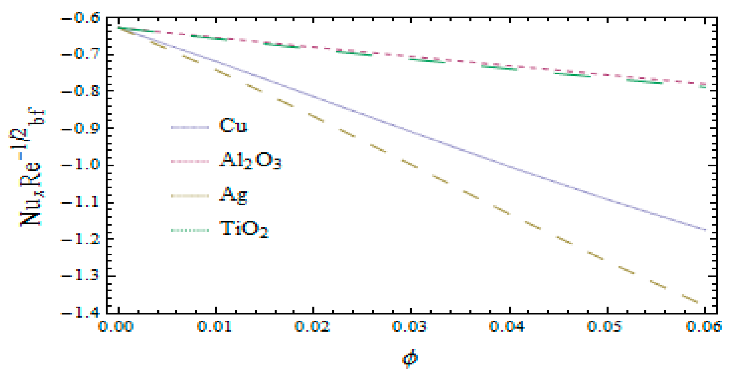
Figure 3 and Figure 4 illustrate the effects of various solid particles and solid volume fraction on CfRe1/2bf and NuxRe−1/2bf, and this change conforms to its mathematical calculation formulas. Nanoparticles cause a change in the thermal conductivity of the mixture, which affects the flow of the fluid. The specific analysis is shown below. The increase in solid volume fraction causes a rise in the heat transfer and the viscosity as well as the resistance of the nanofluids. From the physical meaning of the Nusselt number we could determine that the increase in thermal conductivity led to the decrease in NuxRe−1/2bf. The increase in fluid resistance caused the increase in surface skin friction coefficient in the meantime. In addition, the effect of various solid particles on NuxRe−1/2bf was greater than that of CfRe1/2bf.
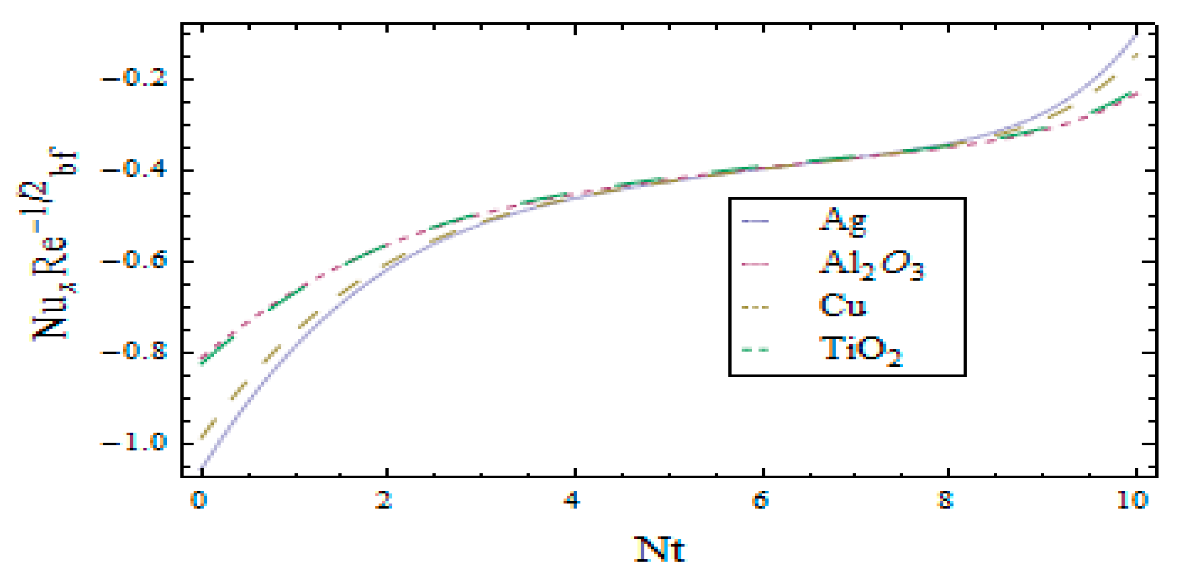
Figure 5 and Figure 6 show the effects of thermophoresis parameter Nt on CfRe1/2bf and NuxRe−1/2bf. Thermophoresis parameter Nt of nano-fluid in the fluid was used to measure the temperature distribution. When the thermophoresis parameter increased, the thermophoretic force helped to migrate the nanoparticles from the region of high temperature to low temperature area, which caused the temperature and the thermal efficiency to rise, resulting in an increase in NuxRe−1/2bf. Nt principally affected NuxRe−1/2bf, and the influence of Nt on CfRe1/2bf only presented a little increase trend. Researchers have shown that velocity slip and temperature jump have a crucial influence on the performance of the fluid at micro or nano scales.
Table 4 demonstrates the effect of the first order and the second order velocity slip and temperature jump on CfRe1/2bf and NuxRe−1/2bf. Velocity slip parameters were used to measure the sliding loss in fluid flow, and the sliding loss affected the velocity by way of the change of fluid flow. With the increase in the first order velocity slip, the wall velocity decreased, which caused the decrease in CfRe1/2bf and NuxRe−1/2bf. With the increase in the second order velocity slip, the result was the the opposite. The temperature jump parameters mainly affected the dimensionless temperature. With the increase in the first order temperature jump, the wall temperature increased. Therefore CfRe1/2bf and NuxRe−1/2bf both decreased. When the temperature of the second order jump is zero, it is a dividing line. When , CfRe1/2bf decreased and NuxRe−1/2bf increased with the rise of the second order temperature jump; but while , CfRe1/2bf rose and NuxRe−1/2bf fell.
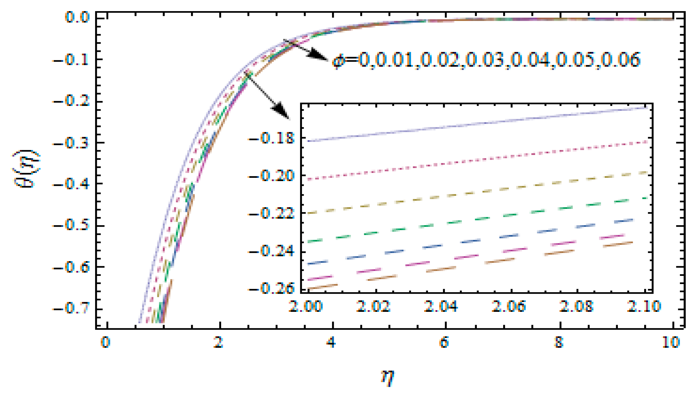
Figure 7 demonstrates the effect of solid volume fraction on dimensionless temperature. When the volume fraction of nanoparticles rose, the thickness of the thermal boundary layer and the thermal conductivity increased, leading to the rise of the wall temperature of the nanofluid. The volume fraction of fluid mainly affected the heat transfer resistance, so the change in speed curve was not very obvious. Figure 8 demonstrates the effect of the thickness of the nanolayer on dimensionless temperature. The thickness of nanolayer primarily affected the solid volume fraction. The solid volume fraction rose with the increase in the thickness of the nanolayer, which gave rise to the decline in wall temperature.
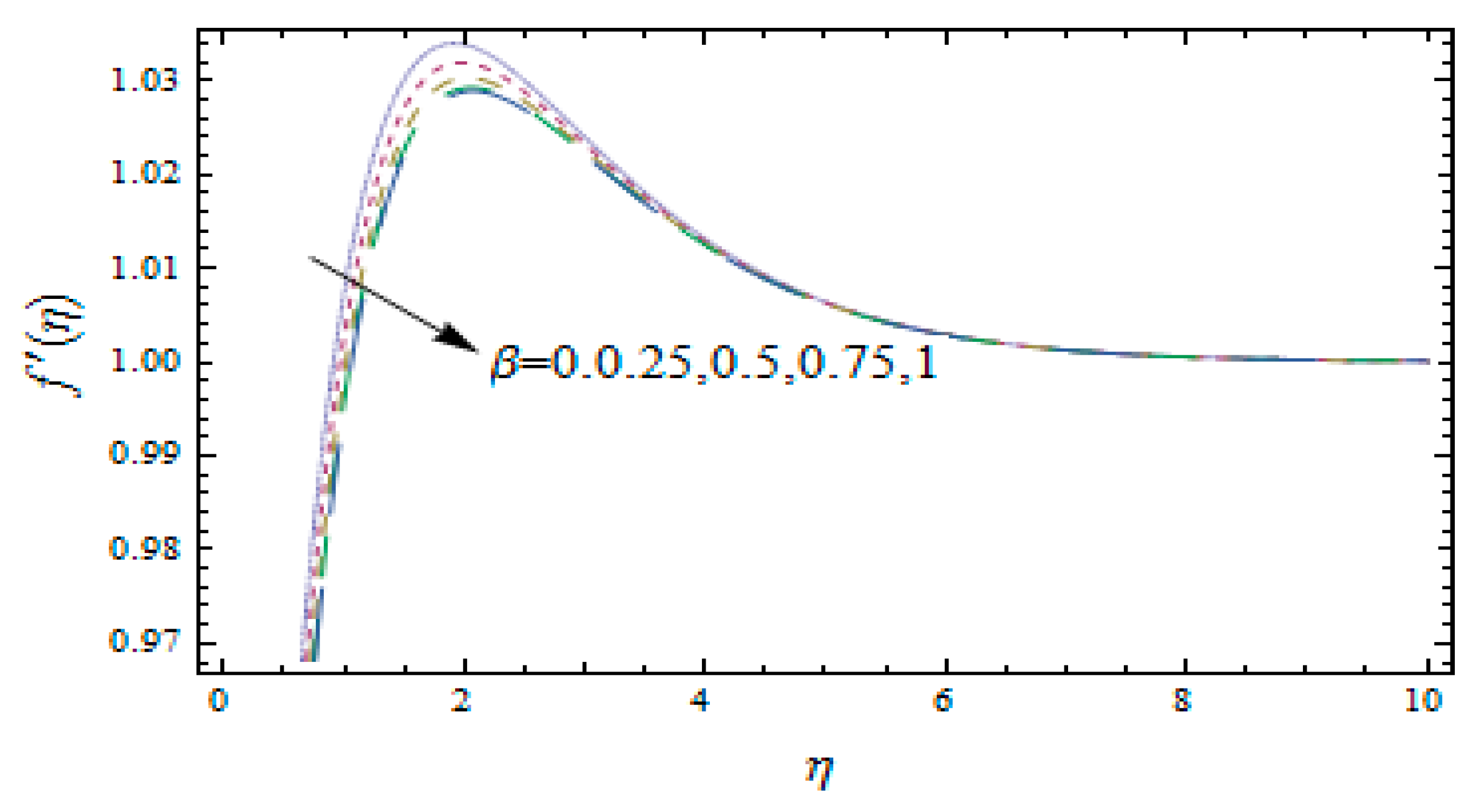
Figure 9 shows the effect of the angle of the wedge on dimensionless velocity. With the increase in the wedge angle, the thermal diffusion reduced, which caused the drop in the temperature of the fluid. This change increased the impact of buoyancy, resulting in the decrease in the driving force of the fluid, which caused the decrease in the fluid velocity. Figure 10 reflects on the dimensionless temperature. The Biot number reflects the distribution of temperature field in the object under unsteady heat conduction. The smaller Bi is, the smaller the internal thermal resistance and the bigger the external thermal resistance. With an increase in Bi, the ratio of the heat resistance increased, which gave rise to the reduction in wall temperature.
4. Conclusions
Considering the effects of the thickness of the nanolayer, temperature jump, and velocity slip, the model of unsteady nanofluid flow and heat transfer was modified in this paper. Meanwhile, both thermophoresis and Brownian motion were considered, and the differential equation was solved by HAM. Some of the main finds of this paper can be summarized as follows:
An increase in the thickness of the nanolayer causes an increase in the local Nussels number NuxRe−1/2bf and the skin friction coefficients CfRe1/2bf, together with the decrease in wall temperature. An enhancement of the thermophoresis parameter gives rise to an increase in NuxRe−1/2bf and CfRe1/2bf.
With an increase in and , CfRe1/2bf and NuxRe−1/2bf reduce. With an increase in the second order velocity slip parameter , the result is the opposite. When the second order temperature jump parameter , CfRe1/2bf decreases and NuxRe−1/2bf increases, with an enhancement of ; but while , CfRe1/2bf rises and NuxRe−1/2bf reduces.
An increase in solid volume fraction causes a decrease in the wall temperature. With an increase in the Biot number the dimensionless wall temperature drops. An increase in the angle of the wedge leads to a decrease in wall velocity.
Author Contributions
J.Z. conducted the original research, modified the model, and contributed analysis tools. J.C. analyzed the data, simulated the modified model, and prepared original draft. J.Z. revised the manuscript.
Funding
This paper was supported by the National Natural Science Foundation of China (No. 11772046; No. 81870345).
Conflicts of Interest
The authors declare no conflict of interest.
References
- Choi, S.U.S. Enhancing thermal conductivity of fluids with nanoparticles. ASME Publ. Fed 1995, 231, 99–106. [Google Scholar]
- Eastman, J.A.; Choi, S.U.S.; Li, S. Anomalously increased effective thermal conductivities of ethylene glycol-based nanofluids containing copper nanoparticles. Appl. Phys. Lett. 2001, 78, 718–720. [Google Scholar] [CrossRef]
- Li, Y.J.; Zhou, J.E.; Tung, S.; Schneider, E.; Xi, S.Q. A review on development of nanofluid preparation and characterization. Powder Technol. 2009, 196, 89–101. [Google Scholar] [CrossRef]
- Yu, W.; Choi, S.U.S. The role of interfacial layers in the enhanced thermal conductivity of nanofluids: A renovated Hamilton–Crosser model. J. Nanopart. Res. 2004, 5, 167–171. [Google Scholar] [CrossRef]
- Azizian, R.; Doroodchi, E.; Moghtaderi, B. Influence of controlled aggregation on thermal conductivity of nanofluids. J. Heat Transf. 2016, 138, 43–55. [Google Scholar] [CrossRef]
- Bigdeli, M.B.; Fasano, M.; Cardellini, A.; Chiavazzo, E.; Asinari, P. A review on the heat and mass transfer phenomena in nanofluid coolants with special focus on automotive applications. Renew. Sustain. Energy Rev. 2016, 60, 1615–1633. [Google Scholar] [CrossRef] [Green Version]
- Fang, T.G. A note on the unsteady boundary layers over a flat plate. Int. J. Non Linear Mech. 2008, 43, 1007–1011. [Google Scholar] [CrossRef]
- Ullah, I.; Shafie, S.; Makinde, O.D.; Khan, I. Unsteady MHD Falkner-Skan flow of Casson nanofluid with generative/destructive chemical reaction. Chem. Eng. Sci. 2017, 172, 694–706. [Google Scholar] [CrossRef]
- Awan, S.E.; Khan, Z.A.; Awais, M.; Rehman, S.U.; Raja, M.A.Z. Numerical treatment for hydro-magnetic unsteady channel flow of nanofluid with heat transfer. Results Phys. 2018, 9, 1543–1554. [Google Scholar] [CrossRef]
- Jahan, S.; Sakidin, H.; Nazar, R.; Pop, I. Unsteady flow and heat transfer past a permeable stretching/shrinking sheet in a nanofluid: A revised model with stability and regression analyses. J. Mol. Liq. 2018, 261, 550–564. [Google Scholar] [CrossRef]
- Hayat, T.; Sajjad, R.; Muhammad, T. On MHD nonlinear stretching flow of Powell–Eyring nanomaterial. Results Phys. 2017, 7, 535–543. [Google Scholar] [CrossRef]
- Tian, X.Y.; Li, B.W.; Hu, Z.M. Convective stagnation point flow of a MHD non-Newtonian nanofluid towards a stretching plate. Int. J. Heat Mass Transf. 2018, 127, 768–780. [Google Scholar] [CrossRef]
- Hsiao, K.L. Combined Electrical MHD Heat Transfer Thermal Extrusion System Using Maxwell Fluid with Radiative and Viscous Dissipation Effects. Appl. Therm. Eng. 2017, 112, 1281–1288. [Google Scholar] [CrossRef]
- Babu, M.J.; Sandeep, N. Three-dimensional MHD slip flow of nanofluids over a slendering stretching sheet with thermophoresis and Brownian motion effects. Adv. Powder Technol. 2016, 27, 2039–2050. [Google Scholar] [CrossRef]
- Usman, M.; Soomro, F.A.; Haq, R.U.; Wang, W.; Defterli, O. Thermal and velocity slip effects on Casson nanofluid flow over an Inclined permeable stretching cylinder via collocation method. Int. J. Heat Mass Transf. 2018, 122, 1255–1263. [Google Scholar] [CrossRef]
- Abbas, N.; Saleem, S.; Nadeem, S.; Alderremy, A.A.; Khan, A.U. On stagnation point flow of a micro polar nanofluid past a circular cylinder with velocity and thermal slip. Results Phys. 2018, 9, 1224–1232. [Google Scholar] [CrossRef]
- Ramzan, M.; Chung, J.D.; Ullah, N. Partial slip effect in the flow of MHD micropolar nanofluid flow due to a rotating disk—A numerical approach. Results Phys. 2017, 7, 3557–3566. [Google Scholar] [CrossRef]
- Seth, G.S.; Mishra, M.K. Analysis of transient flow of MHD nanofluid past a non-linear stretching sheet considering Navier’s slip boundary condition. Adv. Powder Technol. 2017, 28, 375–384. [Google Scholar] [CrossRef]
- Thompson, P.A.; Troian, S.M. A general boundary condition for liquid flow at solid surfaces. Nature 1997, 389, 360–362. [Google Scholar] [CrossRef]
- Zhu, J.; Yang, D.; Zheng, L.C.; Zhang, X.X. Effects of second order velocity slip and nanoparticles migration on flow of Buongiorno nanofluid. Appl. Math. Lett. 2016, 52, 183–191. [Google Scholar] [CrossRef]
- Liu, Q.F.; Zhu, J.; Bandar, B.M.; Zheng, L.C. Hydromagnetic flow and heat transfer with various nanoparticles additives past a wedge with high order velocity slip and temperature jump. Can. J. Phys. 2017, 95, 440–449. [Google Scholar] [CrossRef]
- Sobamowo, M.G.; Jayesimi, L.O.; Waheed, M.A. Magnetohydrodynamic squeezing flow analysis of nanofluid under the effect of slip boundary conditions using variation of parameter method. Karbala Int. J. Mod. Sci. 2018, 4, 107–118. [Google Scholar] [CrossRef]
- Job, V.M.; Gunakala, S.R. Unsteady MHD free convection nanofluid flows within a wavy trapezoidal enclosure with viscous and Joule dissipation effects. Numer. Heat Transf. Appl. 2015, 69, 1–23. [Google Scholar] [CrossRef]
- Liao, S.J. Beyond perturbation: The basic concepts of the homotopy analysis method and its applications. Adv. Mech. 2008, 38, 1–33. [Google Scholar]
- Xie, H.Q.; Fujii, M.; Zhang, X. Effect of interfacial nanolayer on the effective thermal conductivity of nanoparticle-fluid mixture. Int. J. Heat Mass Transf. 2005, 48, 2926–2932. [Google Scholar] [CrossRef]
- Mahalakshmi, T.; Nithyadevi, N.; Oztop, H.F.; Abu-Hamdeh, N. MHD mixed convective heat transfer in a lid-driven enclosure filled with Ag-water nanofluid with center heater. Int. J. Mech. Sci. 2018, 142, 407–419. [Google Scholar] [CrossRef]
- Abdul Hakeem, A.K.; Raja, K.; Ganga, B.; Ganesh, N.V. Nanofluid slip flow through porous medium with elastic deformation and uniform heat source/sink effects. Comput. Therm. Sci. Int. J. 2019, 11, 269–283. [Google Scholar] [CrossRef]
- Rosseland, S. Astrophysik und Atom-Theoretische Grundlagen; Springer: Berlin, Germany, 1931; pp. 41–44. [Google Scholar]
- Kandasamy, R.; Muhaimin, I.; Khamis, A.B. Unsteady Hiemenz flow of Cu-nanofluid over a porous wedge in the presence of thermal stratification due to solar energy radiation: Lie group transformation. Int. J. Therm. Sci. 2013, 65, 196–205. [Google Scholar] [CrossRef]
Figure 1.
hm-.

Figure 2.
hm-.

Figure 3.
The effect of on Nu.

Figure 4.
The effect of on Cf.

Figure 5.
Effect of Nt on Cf.

Figure 6.
The effect of Nt on Nu.

Figure 7.
The effect of on temperature.

Figure 8.
The effect of on temperature.

Figure 9.
The effect of on velocity.

Figure 10.
The effect of on temperature.


Table 1.
The error values of various orders.
| Order | Same hm | Different hm |
|---|---|---|
| 2 | 0.09804597363984649 | 0.10971050115341624 |
| 4 | 0.01695228455734058 | 0.01987321691368215 |
| 6 | 0.00149718658281736 | 0.00111284953763120 |
| 8 | 0.00092006200460696 | 0.00103228583202702 |
| 10 | 0.00016652968112583 | 0.00023106953667965 |
| 12 | 0.00028937817232142 | 0.00018686850247371 |
| 14 | 0.00004625312077364 | 0.00003407739648355 |
| 16 | 0.00004411186515886 | 0.00003247720532823 |
| 18 | 0.00004138348805906 | 0.00003498110747688 |
| 20 | 0.00000913314203849 | 0.00000687359503864 |
Table 2.
The effect of radius on CfRe1/2bf and NuxRe−1/2bf with .
| Radius | NuxRe−1/2bf | CfRe1/2bf |
|---|---|---|
| 5 | −0.891502 | 1.26755 |
| 6 | −0.854912 | 1.24286 |
| 7 | −0.830858 | 1.22730 |
| 8 | −0.813950 | 1.21633 |
| 9 | −0.801466 | 1.20772 |
| 10 | −0.791884 | 1.20219 |
| 11 | −0.784313 | 1.19735 |
| 12 | −0.778192 | 1.19350 |
Table 3.
The effect of the thickness of nanolayer on CfRe1/2bf and NuxRe−1/2bf.
| Thickness | NuxRe−1/2bf | CfRe1/2bf |
|---|---|---|
| 0 | −0.721204 | 1.15796 |
| 1 | −0.747387 | 1.17419 |
| 2 | −0.778192 | 1.1935 |
| 3 | −0.81395 | 1.21633 |
| 4 | −0.854912 | 1.24286 |
| 5 | −0.901176 | 1.27453 |
| 6 | −0.952644 | 1.31082 |
| 7 | −1.00893 | 1.35419 |
| 8 | −1.06935 | 1.40348 |
| 9 | −1.13284 | 1.46137 |
| 10 | −1.19796 | 1.52895 |
Table 4.
The effect of particle and slip parameters on CfRe1/2bf and NuxRe−1/2bf.
| Parameter | Value | NuxRe−1/2bf | CfRe1/2bf |
|---|---|---|---|
| 0 | −0.739726 | 1.279140 | |
| 0.5 | −0.737890 | 0.987631 | |
| 1 | −0.736706 | 0.810298 | |
| 1.5 | −0.735953 | 0.678731 | |
| 2 | −0.735382 | 0.586453 | |
| −1 | −0.736851 | 0.829446 | |
| −0.5 | −0.739202 | 1.184720 | |
| 0 | −0.744404 | 1.996120 | |
| 0.3 | −0.752506 | 3.308360 | |
| 0.5 | −0.767527 | 5.848600 | |
| 0 | −1.060260 | 0.944702 | |
| 1 | −0.471135 | 0.944367 | |
| 2 | −0.407875 | 0.944307 | |
| 3 | −0.302604 | 0.944202 | |
| −2 | −0.210557 | 0.918785 | |
| −1 | −0.372054 | 0.918769 | |
| −0.5 | −0.603914 | 0.918768 | |
| 0 | −1.839810 | 0.916633 | |
| 0.5 | 2.405830 | 0.914590 | |
| 1 | 0.681384 | 0.918776 | |
| 2 | 0.294131 | 0.918839 |
© 2019 by the authors. Licensee MDPI, Basel, Switzerland. This article is an open access article distributed under the terms and conditions of the Creative Commons Attribution (CC BY) license (http://creativecommons.org/licenses/by/4.0/).
Share and Cite
MDPI and ACS Style
Zhu, J.; Cao, J. Effects of Nanolayer and Second Order Slip on Unsteady Nanofluid Flow Past a Wedge. Mathematics 2019, 7, 1043. https://doi.org/10.3390/math7111043
AMA Style
Zhu J, Cao J. Effects of Nanolayer and Second Order Slip on Unsteady Nanofluid Flow Past a Wedge. Mathematics. 2019; 7(11):1043. https://doi.org/10.3390/math7111043
Chicago/Turabian StyleZhu, Jing, and Jiahui Cao. 2019. "Effects of Nanolayer and Second Order Slip on Unsteady Nanofluid Flow Past a Wedge" Mathematics 7, no. 11: 1043. https://doi.org/10.3390/math7111043
Note that from the first issue of 2016, this journal uses article numbers instead of page numbers. See further details here.