A Fractional-Order Predator–Prey Model with Ratio-Dependent Functional Response and Linear Harvesting

Abstract

We consider a model of predator–prey interaction at fractional-order where the predation obeys the ratio-dependent functional response and the prey is linearly harvested. For the proposed model, we show the existence, uniqueness, non-negativity and boundedness of the solutions. Conditions for the existence of all possible equilibrium points and their stability criteria, both locally and globally, are also investigated. The local stability conditions are derived using the Magtinon’s theorem, while the global stability is proven by formulating an appropriate Lyapunov function. The occurrence of Hopf bifurcation around the interior point is also shown analytically. At the end, we implemented the Predictor–Corrector scheme to perform some numerical simulations.

1. Introduction

One of interesting topics in ecological systems is the predator–prey model, which studies the dynamics of the populations as the extinction conditions of populations, and terms of its existence as the result of their interaction. A general Lotka–Volterra prey–predator model is given by

$$\begin{array}{ccc}{\displaystyle \frac{du}{dt}}& =& {\displaystyle ru\left(1-\frac{u}{K}\right)-p\left(u\right)v,}\hfill \\ {\displaystyle \frac{dv}{dt}}& =& {\displaystyle np\left(u\right)v-dv,}\hfill \end{array}$$

(1)

where u and v, respectively, represent the population of prey and predator, $p\left(u\right)$ denotes the functional response, and n is the conversion rate of predation into predator growth rate. r, K and d are the prey intrinsic growth rate, the prey carrying capacity and the predator death rate, respectively. The model in Equation (1) was proposed by Gause et al. [1].

In modeling the interaction between predator and prey, one important task is to determine the specific form of functional response [2], so the model is relevant to the expected ecological conditions. For example, Rosenzweig and MacArthur [3] considered a Michaelis–Menten functional response (also known as Holling Type II functional response) ${\displaystyle p\left(u\right)=\frac{mu}{\omega +u}}$. This specific functional response assumes that the prey population is a limited resource and that predation converges to a constant when the population of prey increases. Here, m and $\omega$ are the capturing rate of prey by predator and the half saturation constant, respectively. Since the value of $p\left(u\right)$ is fluctuated by prey density, this functional response is called by “prey-dependence”. Several researchers argue that the functional response depends not only on prey, but also on the ratio of both populations [2,4,5,6], known also as “ratio-dependent” functional response. Such functional response is defined by $p\left(\frac{u}{v}\right)$. Recently, Xiao and Cao [7] studied the interaction of prey and predator with a ratio-dependent functional response with linear harvesting for both prey and predator population:

$$\begin{array}{ccc}{\displaystyle \frac{du}{dt}}& =& {\displaystyle ru\left(1-\frac{u}{K}\right)-\frac{muv}{u+\omega v}-k_{1}u,}\hfill \\ {\displaystyle \frac{dv}{dt}}& =& {\displaystyle \frac{nuv}{u+\omega v}-dv-k_{2}v.}\hfill \end{array}$$

(2)

Using the following transformation

$$(u,v,t)\to \left(\frac{u}{K},\frac{\omega v}{K},rt\right),$$

the model in Equation (2) can be simplified as

$$\begin{array}{ccc}{\displaystyle \frac{du}{dt}}& =& {\displaystyle u(1-u)-\frac{auv}{u+v}-ku,}\hfill \\ {\displaystyle \frac{dv}{dt}}& =& {\displaystyle \frac{buv}{u+v}-\delta v,}\hfill \end{array}$$

(3)

where

$$a=\frac{m}{r},k=\frac{k_1}{r},b=\frac{n}{\omega },\delta =\frac{1}{r\omega }(d+k_2),a,k,b,\delta >0.$$

Note that the prey and predator growth rates in the model in Equation (3) only depend on the current conditions. In fact, the growth rates of population also depend on long-time memory. To include such memory effects, many researchers have applied fractional derivatives to get fractional differential equations. There are various theories of fractional derivatives in the literature. Among many, two well known fractional derivatives are Riemann–Liouville and Caputo. We consider here the Caputo fractional derivative since the classical initial values as in the differential equations of integer order can also be applied.

Definition 1.

[8] Suppose$\alpha >0$. The fractional operator

$$D_{*}^{\alpha }g\left(t\right)=\frac{1}{\Gamma (n-\alpha )}{\int }_0^t\frac{g^{\left(n\right)}\left(s\right)}{{(t-s)}^{1+\alpha -n}}ds,$$

is called the Caputo fractional derivative of order α, where$n=\lceil \alpha \rceil$. Particularly, if$\alpha \in (0,1]$, then we have

$$D_{*}^{\alpha }g\left(t\right)=\frac{1}{\Gamma (1-\alpha )}{\int }_{t_0}^t\frac{g^{\prime }\left(s\right)}{{(t-s)}^{\alpha }}ds.$$

Note that the Caputo operator is nonlocal operator, i.e., includes the history from initial state to the current state. Therefore, the Caputo fractional derivative is often applied in modeling biological systems to describe the influence of memory effects (see, e.g., [9,10,11,12,13]). Biologically, the growth rates of both prey and predator not only depend on the current conditions, but also depend on all previous conditions. To model such long-time memory effects, the first derivatives of the system in Equation (3) are replaced by the Caputo derivative as follows

$$\begin{array}{ccc}{D}_{*}^{\alpha }u\left(t\right)& =& {\displaystyle u(1-u)-\frac{auv}{u+v}-ku,}\hfill \\ D_{*}^{\alpha }v\left(t\right)& =& {\displaystyle \frac{buv}{u+v}-\delta v.}\hfill \end{array}$$

(4)

We assume that the initial conditions are $u\left(0\right)=u_0>0$ and $v\left(0\right)=v_0>0$ where $\alpha \in (0,1]$. Further, we consider $0<k<1$ as the harvesting parameter.

Notice that the model in Equation (4) is a system of nonlinear fractional differential equations and finding an analytical solution of such nonlinear system can be very complicated. In the case of some nonlinear ordinary differential system, Shang [14,15,16] introduced the Lie algebra approach to obtain exact solutions. The exact solutions of some nonlinear fractional differential equations may also be found using similar method (see, for example, [17,18]). In the Lie algebra method, the solution is constructed from the symmetry property of the model. Since the mathematical model of biological system is often complicated and the symmetry is lacking, this method is not widely implemented. An example application is the effect of microtemperatures for micropolar thermoelastic bodies [19].

In this paper, we are not interested in finding analytical solutions of the system in Equation (4) but we more focus on the dynamics of this system. The local stability of the system in Equation (4) without harvesting was investigated by Suryanto and Darti [20]. However, the dynamics of the full system in Equation (4), to the best of our knowledge, has not been investigated. Thus, a fractional-order ratio-dependent predator–prey model with linear harvesting is proposed and the dynamical behavior of the model is studied. We first show the existence, uniqueness, boundedness and non-negativity of solutions of the system in Equation (4). The stability analysis of equilibrium points is performed both locally using Matignon’s Theorem and globally by choosing suitable Lyapunov function. From the local analysis, we also prove the existence of Hopf bifurcation driven the order of fractional derivative. Then, we implement a predictor–corrector scheme to do numerical simulations and to illustrate our analytical findings. The focus of numerical simulations was to study the effects of fractional-order $\left(\alpha \right)$ and the harvesting coefficient. We show that smaller $\alpha$ stabilizes the equilibrium points as its stability region is larger. To study the dynamical behavior of the system in Equation (4), we first introduce some basic concepts of fractional differential equations.

2. Preliminaries

The following lemma is needed to prove the existence and uniqueness of the solution for the system in Equation (4).

Lemma 1.

(See [21]). Consider a fractional-order-system

$$D_{*}^{\alpha }u\left(t\right)=f(t,u\left(t\right)),t>0,u\left(0\right)\ge 0,\alpha \in (0,1],$$

(5)

where$f:(0,\infty )\times \Omega \to {\mathbb{R}}^n,\Omega \subseteq {\mathbb{R}}^n$. A unique solution of Equation (5) on$(0,\infty )\times \Omega$exists if$f(t,u(t\left)\right)$satisfies the locally lipschitz condition with respect to u.

To prove the non-negativity of the solution for the system in Equation (4), the following lemma and corollary are needed.

Lemma 2.

(See [22]). Assume that$u\left(t\right)\in C[0,c]$,$D_{*}^{\alpha }u\left(t\right)\in C[0,c]$and$\alpha \in (0,1]$. Then, we get

$$u\left(t\right)=u\left(0\right)+\frac{1}{\Gamma \left(\alpha \right)}{D}_{*}^{\alpha }u\left(\xi \right)t^{\alpha },$$

(6)

where$0\le \xi \le x,\forall x\in (0,c]$.

Corollary 1.

(See [22]). Assume that$u\left(t\right)\in C[0,c]$,$D_{*}^{\alpha }u\left(t\right)\in C[0,c]$and$\alpha \in (0,1]$. If$D_{*}^{\alpha }u\left(t\right)\ge 0$,$\forall t\in (0,c)$, then$u\left(t\right)$is a non-decreasing function for all$t\in [0,c]$. If$D_{*}^{\alpha }u\left(t\right)\le 0,\forall t\in (0,c)$, then$u\left(t\right)$is a non-increasing function for all$t\in [0,c]$.

The following comparison theorem is important to show the uniform boundedness of the solution.

Theorem 1.

(Comparison Theorem [23]). Let$u\left(t\right)\in C\left([0,+\infty )\right)$. If$u\left(t\right)$satisfies

$$\begin{array}{c}{D}_{*}^{\alpha }u\left(t\right)\le -\lambda u\left(t\right)+\mu ,u\left(0\right)=u_0\in \mathbb{R},\end{array}$$

where$\alpha \in (0,1],\lambda ,\mu \in \mathbb{R}$and$\lambda \ne 0$, then

$$u\left(t\right)\le \left(u_0-\frac{\mu }{\lambda }\right)E_{\alpha }[-\lambda t^{\alpha }]+\frac{\mu }{\lambda },$$

where$E_{\alpha }\left(z\right)$is the Mittag–Leffler function of one parameter, which is defined by

$$E_{\alpha }\left(z\right)=\sum _{j=1}^{\infty }\frac{z^j}{\Gamma (\alpha j+1)}.$$

This function plays a crucial role in the classical calculus for $\alpha =1$, where it becomes the exponential function, that is

$$e^z=E_1\left(z\right)=\sum _{j=1}^{\infty }\frac{z^j}{\Gamma (j+1)}.$$

In [24], the fractional derivatives of Mittag–Leffler functions and further several important properties were established. The relationships between the Mittag–Leffler and Wright functions were also proved [24].

Theorem 2.

(See [25,26]). Consider an autonomous nonlinear fractional-order system

$$D_{*}^{\alpha }\overrightarrow{u}=\overrightarrow{f}(\overrightarrow{u});\overrightarrow{u}\left(0\right)={\overrightarrow{u}}_0;\alpha \in (0,1].$$

A point${\overrightarrow{u}}^{*}$is called an equilibrium point of the system if it satisfies$\overrightarrow{f}({\overrightarrow{u}}^{*})=0$. This equilibrium point is locally asymptotically stable if all eigenvalues${\lambda }_j$of the Jacobian matrix$J=\frac{\partial f}{\partial u}$evaluated at${\overrightarrow{u}}^{*}$satisfy$|arg\left({\lambda }_j\right)|>\frac{\alpha \pi }{2}$.

Lemma 3.

[27] Let$u\left(t\right)\in C\left({\mathbb{R}}_{+}\right)$and its fractional derivatives of order α exist for any$\alpha \in (0,1]$. Then, for any$t>0$, we have

$$D_{*}^{\alpha }\left[u\left(t\right)-u^{*}-u^{*}ln\frac{u\left(t\right)}{u^{*}}\right]\le \left(1-\frac{u^{*}}{u\left(t\right)}\right)D_{*}^{\alpha }u\left(t\right),u^{*}\in {\mathbb{R}}_{+}.$$

Lemma 4.

(Generalized Lasalle Invariance Principle [28]). Suppose Ω is a bounded closed set and every solution of

$$D_{*}^{\alpha }u\left(t\right)=f\left(u\left(t\right)\right),$$

starts from a point in Ω and remains in Ω for all time. If$\exists V\left(u\right):\Omega \to \mathbb{R}$with continuous first partial derivatives satisfies

$$D_{*}^{\alpha }{V|}_{D_{*}^{\alpha }u\left(t\right)=f\left(u\left(t\right)\right)}\le 0.$$

Let$E:=\left\{u|D_{*}^{\alpha }{V|}_{D_{*}^{\alpha }u\left(t\right)=f\left(u\left(t\right)\right)}=0\right\}$and M be the largest invariant set of E. Then, every solution$u\left(t\right)$originating in Ω tends to M as$t\to \infty$.

Function $V\left(u\right)$ in Lemma 4 is termed as a Lyapunov function. To apply this lemma, we need to construct a suitable Lyapunov function for the considered fractional system that satisfies Lemma 4 and show that the equilibrium point is the largest invariant set of E. Here, we usually need Lemma 3 to prove the non-positivity of the partial derivatives of the Lyapunov function.

3. Main Results

3.1. Existence and Uniqueness

In this section, we investigate the existence and uniqueness of solution of the fractional-order system in Equation (4) in the region $[0,\infty )\times {\Omega }_M$ where

$${\Omega }_M=\left\{\left(u,v\right)\in {\mathbb{R}}^2:max\left\{\left|u\right|,\left|v\right|\right\}\le \gamma \right\},$$

for sufficiently large $\gamma$. The existence of $\gamma$ is guaranteed by the boundedness of the solution, which is shown below. We first denote $Y=\left(u,v\right)$ and $\overline{Y}=\left(\overline{u}.\overline{v}\right)$, and then consider a mapping $F\left(Y\right)=\left(F_1\left(Y\right),F_2\left(Y\right)\right)$ where

$$\begin{array}{cc}\hfill F_1\left(Y\right)& =u(1-u)-\frac{auv}{u+v}-ku,\hfill \\ \hfill F_2\left(Y\right)& =\frac{buv}{u+v}-\delta v.\hfill \end{array}$$

For any $Y,\overline{Y}\in {\Omega }_M$, next we show that

$$\begin{array}{ccc}∥F\left(Y\right)-F\left(\overline{Y}\right)∥& =& \left|F_1\left(Y\right)-F_1\left(\overline{Y}\right)\right|+\left|F_2\left(Y\right)-F_2\left(\overline{Y}\right)\right|\hfill \\ & =& {\displaystyle \left|u(1-u)-\frac{auv}{u+v}-ku-\overline{u}(1-\overline{u})+\frac{a\overline{u}\overline{v}}{\overline{u}+\overline{v}}+k\overline{u}\right|}\hfill \\ & & {\displaystyle +\left|\frac{buv}{u+v}-\delta v-\frac{b\overline{u}\overline{v}}{\overline{u}+\overline{v}}+\delta \overline{v}\right|}\hfill \\ & =& {\displaystyle \left|\left(1-k\right)\left(u-\overline{u}\right)-\left(u+\overline{u}\right)\left(u-\overline{u}\right)-a\frac{u\overline{u}\left(v-\overline{v}\right)+v\overline{v}\left(u-\overline{u}\right)}{\left(u+v\right)\left(\overline{u}+\overline{v}\right)}\right|}\hfill \\ & & {\displaystyle +\left|b\frac{u\overline{u}\left(v-\overline{v}\right)+v\overline{v}\left(u-\overline{u}\right)}{\left(u+v\right)\left(\overline{u}+\overline{v}\right)}-\delta \left(v-\overline{v}\right)\right|.}\hfill \end{array}$$

By applying the triangle inequality $\left|u_1\pm u_2\right|\le \left|u_1\right|+\left|u_2\right|$, and noticing that $max\left\{\left|u\right|,\left|v\right|\right\}\le \gamma$ and ${\displaystyle \left|\frac{u\overline{u}}{\left(u+v\right)\left(\overline{u}+\overline{v}\right)}\right|\le 1}$, we can show that

$$\begin{array}{ccc}∥F\left(Y\right)-F\left(\overline{Y}\right)∥& \le & {\displaystyle \left(1-k\right)\left|u-\overline{u}\right|+2\gamma \left|u-\overline{u}\right|+\left(a+b\right)\left|\frac{v\overline{v}}{\left(u+v\right)\left(\overline{u}+\overline{v}\right)}\right|\left|u-\overline{u}\right|}\hfill \\ & & {\displaystyle +\left(a+b\right)\left|\frac{u\overline{u}}{\left(u+v\right)\left(\overline{u}+\overline{v}\right)}\right|\left|v-\overline{v}\right|+\delta \left|v-\overline{v}\right|}\hfill \\ & \le & \left(1-k+2\gamma +a+b\right)\left|u-\overline{u}\right|+\left(a+b+\delta \right)\left|v-\overline{v}\right|\hfill \\ & \le & L∥Y-\overline{Y}∥,\hfill \end{array}$$

where $L=max\left\{1-k+2\gamma +a+b,a+b+\delta \right\}$. Hence, $F\left(Y\right)$ satisfies the Lipschitz condition. By Lemma 1, the fractional-order system in Equation (4) with initial values $Y_0=\left(u_0,v_0\right)$ where $u_0\ge 0$ and $v_0\ge 0$ has a unique solution $Y\left(t\right)=\left(u\left(t\right),v\left(t\right)\right)\in {\Omega }_M$. Thus, we establish the following existence and uniqueness of solution of the system in Equation (4).

Theorem 3.

The fractional-order predator–prey system in Equation (4) subject to any non-negative initial value$\left(u_0,v_0\right)$has a unique solution$\left(u\left(t\right),v\left(t\right)\right)\in {\Omega }_M$for all$t>0$.

3.2. Boundedness and Non-Negativity

The system in Equation (4) describes the interaction of prey population with predator population at fractional-order and therefore solutions of this system must be bounded and non-negative. Let

$${\Omega }_{+}:=\left\{(u,v)|u\ge 0\mathrm{and}v\ge 0\right\},$$

denotes all non-negative real number in ${\mathbb{R}}^2$. The non-negativity and boundedness of solutions of the system in Equation (4) are guaranteed by the following theorem.

Theorem 4.

All solutions of the system in Equation (4) with$u_0>0$and$v_0>0$are uniformly bounded and non-negative.

Proof. 

We first assume $u_0>0$ and $v_0>0$ and show that $u\left(t\right)\ge 0,\forall t>0$. Suppose that is not correct, then we can find $t_1>0$ such that $u\left(t\right)>0$ for $t\in [0,t_1),u\left(t_1\right)=0$ and $u\left(t\right)<0$ for $t>t_1$. From the first equation in the system in Equation (4), we obtain

$$\begin{array}{c}\hfill D_{*}^{\alpha }u\left(t\right){\mid }_{t=t_1}=0.\end{array}$$

Based on Corollary 1, we get $u\left(t_1^{+}\right)=0$, which contradicts the fact $u\left(t_1^{+}\right)<0$, i.e., $u\left(t\right)<0,\forall t>t_1$. Hence, we get $u\left(t\right)\ge 0,\forall t\ge 0$. Using the same arguments, we can show that $v\left(t\right)\ge 0,\forall t\ge 0$. We next prove that all solutions of the system in Equation (4) are uniformly bounded. For that, we define a function $w=u+\frac{a}{b}v$. From the system in Equation (4), we obtain

$$\begin{array}{cc}\hfill D_{*}^{\alpha }w+\delta w& =u\left(1-u\right)-\frac{auv}{u+v}-ku+\frac{auv}{u+v}-\frac{a\delta }{b}v+\delta u+\frac{a\delta }{b}v\hfill \\ \hfill & =-u^2+\left(1-k+\delta \right)u\hfill \\ \hfill & =-{\left(u-\frac{1-k+\delta }{2}\right)}^2+\frac{{\left(1-k+\delta \right)}^2}{4}\hfill \\ \hfill & \le \frac{{\left(1-k+\delta \right)}^2}{4}.\hfill \end{array}$$

Based on the comparison in Theorem 1, we obtain

$$w\left(t\right)\le \left(w\left(0\right)-\frac{{\left(1-k+\delta \right)}^2}{4\delta }\right)E_{\alpha }\left(-\delta t^{\alpha }\right)+\frac{{\left(1-k+\delta \right)}^2}{4\delta },$$

where $E_{\alpha }$ is the Mittag–Leffler function. Since

$$E_{\alpha }\left(-\delta t^{\alpha }\right)⟶0ast⟶\infty ,$$

(see [29], Lemma 5 and Corollary 6), we have

$$w\left(t\right)\le \frac{{\left(1-k+\delta \right)}^2}{4\delta },t⟶\infty .$$

Hence, all solutions of the system in Equation (4), which start in $R_{+}^2$, are restricted to the region ${\Omega }_B$ where

$${\Omega }_B=\left\{\left(u,v\right)\in {\mathbb{R}}_{+}^2:u+\frac{a}{b}v\le \frac{{\left(1-k+\delta \right)}^2}{4\delta }+\epsilon ,\epsilon >0\right\}.$$

(7)

Thus, all solutions of fractional-order system in Equation (4) are uniformly bounded. □

3.3. Local Stability

Based on Theorem (2), we can show that the system in Equation (4) has three equilibrium points as follows:

• The extinction point of both prey and predator population $E_0=\left(0,0\right)$ which is always feasible.
• The free predator point $E_1=\left(k_0,0\right)$, which also always exists. Here, $k_0=1-k$.
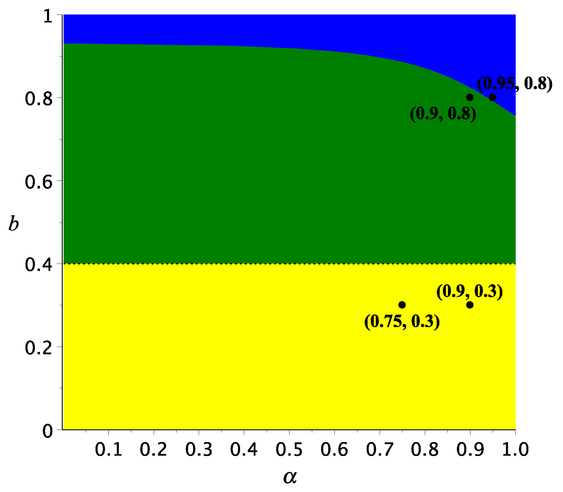
• The interior point $E^{*}=\left(u^{*},v^{*}\right)$ where $u^{*}=\frac{1}{b}\left(b{k}_0-a\left(b-\delta \right)\right)$ and $v^{*}=\frac{1}{\delta }\left(b-\delta \right)u^{*}$. Notice that $E^{*}$ exists if $0<\left(b-\delta \right)<\frac{b}{a}{k}_0$.

In the following, we study the dynamics of the system in Equation (4) around each of equilibrium point. For that, we linearize the system in Equation (4) around each equilibrium point. The Jacobian matrix obtained from this linearization at an equilibrium point $E(u,v)$ is given by

$$J\left(E\right)=\left[\begin{array}{cc}\frac{\partial F_1}{\partial u}& \frac{\partial F_1}{\partial v}\\ \frac{\partial F_2}{\partial u}& \frac{\partial F_2}{\partial v}\end{array}\right]=\left[\begin{array}{cc}{k}_0-2u-\frac{a{v}^2}{{\left(u+v\right)}^2}& -\frac{a{u}^2}{{\left(u+v\right)}^2}\\ \frac{b{v}^2}{{\left(u+v\right)}^2}& \frac{b{u}^2}{{\left(u+v\right)}^2}-\delta \end{array}\right],$$

(8)

where $F_1$ and $F_2$ are as in Section 3.1. By evaluating this Jacobian matrix at each equilibrium points and applying Theorem 2, we obtain the stability properties of $E_0$ and $E_1$ as follows.

Theorem 5.

For the fractional-order system in Equation (4), the extinction of both population point$\left(E_0\right)$and the free predator point$\left(E_1\right)$have the following stability properties.

1. 

$E_0$is a saddle point.

2. 

If$b<\delta$, then$E_1$is locally asymptotically stable and it is a saddle if$b>\delta$.

Proof. 

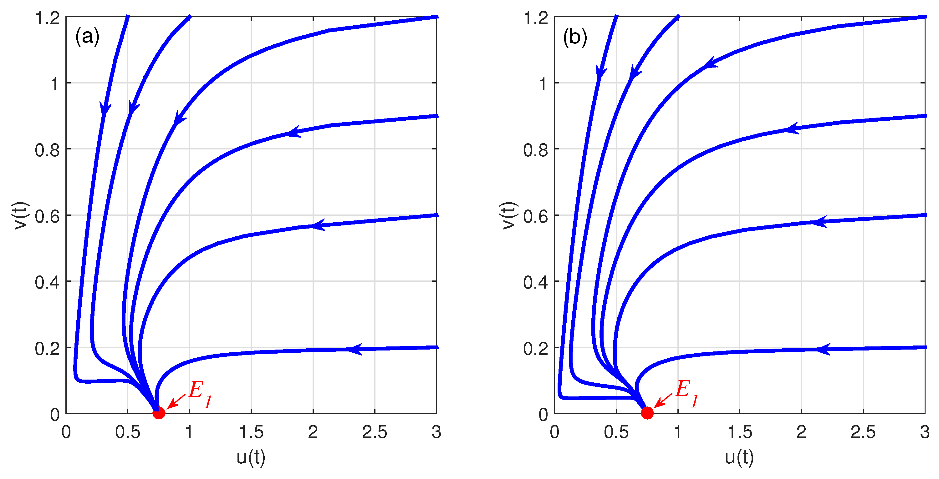
• The Jacobian matrix in Equation (8) evaluated at $E_0$ is

  $$J\left(E_0\right)=\left[\begin{array}{cc}{k}_0& 0\\ 0& -\delta \end{array}\right].$$
  The eigenvalues of $J\left(E_0\right)$ are ${\lambda }_1=k_0>0$ and ${\lambda }_2=-\delta <0$, and consequently we have $\left|arg\left({\lambda }_1\right)\right|=0<\alpha \pi /2$ and $\left|arg\left({\lambda }_2\right)\right|=\pi >\alpha \pi /2$ for $0<\alpha <1$. Hence, $E_0$ is a saddle point.
• If $E_1$ is substituted into the Jacobian matrix in Equation (8), then we have

  $$J\left(E_1\right)=\left[\begin{array}{cc}-k_0& -a\\ 0& b-\delta \end{array}\right].$$
  Obviously, $J\left(E_1\right)$ has eigenvalues ${\lambda }_1=-k_0<0$ and ${\lambda }_2=b-\delta$. We observe that $\left|arg\left({\lambda }_1\right)\right|=\pi >\alpha \pi /2$. If $b<\delta$, then ${\lambda }_2<0$ and thus $\left|arg\left({\lambda }_2\right)\right|=\pi >\alpha \pi /2$. On the other hand, if $b>\delta$, then ${\lambda }_2>0$, and consequently $\left|arg\left({\lambda }_2\right)\right|=0<\alpha \pi /2$. Therefore, $E_1$ is asymptotically stable (locally) if $b<\delta$ and is a saddle point if $b>\delta$.

 □

A similar idea for fractional version is also applied in the percolation theory (see [30]).

We now examine the stability of equilibrium $E^{*}$. The characteristics equation of the Jacobian matrix evaluated at $E^{*}$ is given by

$${\lambda }^2-T\lambda +D=0,$$

(9)

where $T=-\left(b^2{k}_0+b^2\left(\delta -a\right)+{\delta }^2\left(a-b\right)\right)/b^2$ and $D=\left(b\delta k_0\left(b-\delta \right)-a\delta {\left(b-\delta \right)}^2\right)/b^2$. From the existence condition of $E^{*}$, we notice that $D>0$. The eigenvalues of $J\left(E^{*}\right)$ is

$${\lambda }_{1,2}=\frac{T\pm \sqrt{\Delta }}{2},\Delta =T^2-4D.$$

By analyzing these eigenvalues, the stability of $E^{*}$ is stated in following theorem.

Theorem 6.

For the fractional-order system in Equation (4), the interior point$E^{*}$is locally asymptotically stable if one of the following mutually exclusive conditions holds:

1. 

$T<0$and$\Delta \ge 0$

2. 

$\Delta <0$and$\frac{\sqrt{\left|\Delta \right|}}{T}>tan\left(\frac{\alpha \pi }{2}\right)$.

Proof. 

• Since $D>0,T<0$ and $\Delta \ge 0$, ${\lambda }_{1,2}<0$ and $arg\left({\lambda }_{1,2}\right)=\pi >\alpha \pi /2$. Therefore, $E^{*}$ is asymptotically stable.
• Suppose $\Delta <0$. If $\lambda$ is an eigenvalue, then its complex conjugate $\left(\overline{\lambda }\right)$ is also an eigenvalue. We have that $\left|\frac{\lambda -\overline{\lambda }}{\lambda +\overline{\lambda }}\right|=\left|\frac{Im\left(\lambda \right)}{Re\left(\lambda \right)}\right|=arg\left(\lambda \right)=\frac{\sqrt{\left|\Delta \right|}}{T}$. Using the Matignon’s condition (see Theorem 2), it is obvious that $E^{*}$ is locally asymptotically stable if $\frac{\sqrt{\left|\Delta \right|}}{T}>tan\left(\frac{\alpha \pi }{2}\right)$.

 □

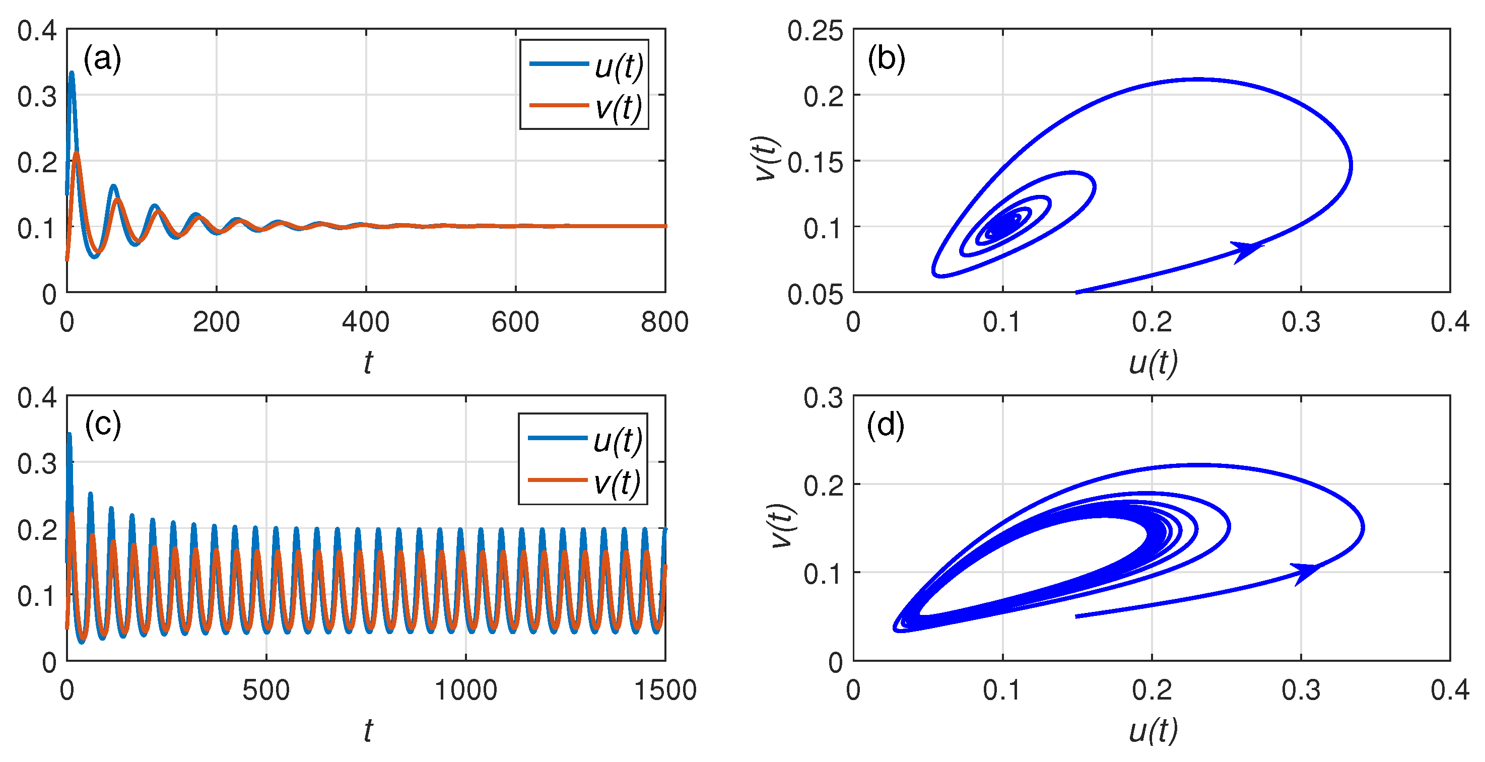
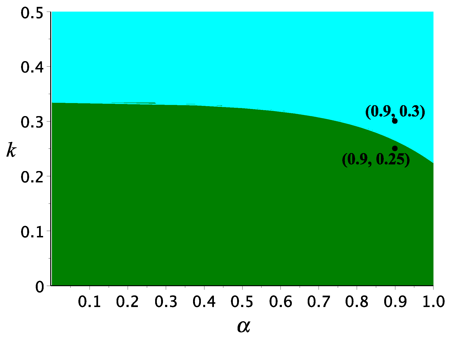
3.4. Hopf Bifurcation

For the following fractional-order commensurate system:

$$D_{*}^{\alpha }w=f(\mu ,w),\alpha \in (0,1],w\in {\mathbb{R}}^2,$$

(10)

Abdelouahab et al. [31] stated that a Hopf bifurcation occurs around an equilibrium E at $\mu ={\mu }^{*}$ if the following conditions hold:

(i)

The eigenvalues of the Jacobian matrix are a pair of complex-conjugate: ${\lambda }_{1,2}\left(\mu \right)=\zeta \left(\mu \right)\pm i\omega \left(\mu \right)$;

(ii)

$p_{1,2}(\alpha ,{\mu }^{*})=0$; and

(iii)

$\frac{\partial p_{1,2}}{\partial \mu }{|}_{\mu ={\mu }^{*}}\ne 0,$

where $p_j(\alpha ,\mu )=\frac{\alpha \pi }{2}-|arg\left({\lambda }_j\left(\mu \right)\right)|,j=1,2.$

The existence of a Hopf bifurcation in the system in Equation (4) is analyzed as follows. From Theorem 6, we can derive the following theorem.

Theorem 7.

Suppose$\Delta <0$and$T>0$. The fractional the model in Equation (4) undergoes a Hopf bifurcation at$E^{*}$when the fractional-order α crosses the critical values

$${\alpha }^{*}=\frac{2}{\pi }{tan}^{-1}\left(\frac{\sqrt{|\Delta |}}{T}\right).$$

Proof. 

If $\Delta <0$, $T>0$ and $\alpha ={\alpha }^{*}$, then the characteristic equation of the Jacobian matrix at $E^{*}$ has a pair of conjugate complex roots ${\lambda }_{1,2}$ located on the border of stability area $arg\left({\lambda }_{1,2}\right)=\frac{{\alpha }^{*}\pi }{2}$. If $\alpha$ changes around ${\alpha }^{*}$, ${\lambda }_{1,2}$ pass through the stability margin and a Hopf bifurcation occurs. □

3.5. Global Asymptotic Stability

Theorem 8.

Let$k_0=1-k$.$E_1$is globally asymptotically stable in the region${\Omega }_1=\left\{(u,v)|u+v\ge \frac{b{k}_0}{\delta }\right\}$.

Proof. 

Define a Lyapunov function $\mathcal{U}(u,v)=\left(u-k_0-k_{0}ln\frac{u}{k_0}+\frac{a}{b}v\right)$. Using Lemma 3, we can show

$$\begin{array}{ccc}{D}_{*}^{\alpha }\mathcal{U}(u,v)& \le & {\displaystyle \frac{u-k_0}{u}{D}_{*}^{\alpha }u+\frac{a}{b}{D}_{*}^{\alpha }v}\hfill \\ & =& {\displaystyle (u-k_0)\left[k_0-u-a\frac{v}{u+v}\right]+\frac{a}{b}\left(b\frac{u}{u+v}-\delta \right)v}\hfill \\ & =& {\displaystyle -{(u-k_0)}^2+a\left[\frac{k_0}{u+v}-\frac{\delta }{b}\right]v.}\hfill \end{array}$$

It is obvious that $D_{*}^{\alpha }\mathcal{U}(u,v)\le 0,\forall (u,v)\in {\Omega }_1$. Furthermore, $D_{*}^{\alpha }\mathcal{U}(u,v)=0$ implies that $u=k_0$ and $v=0$. Hence, the only invariant set on which $D_{*}^{\alpha }\mathcal{U}(u,v)=0$ is the singleton $\left\{E_1\right\}$. Using Lasalle invariance principle (Lemma 4), we conclude that $E_1$ is globally asymptotically stable. □

Theorem 9.

$E^{*}$is globally asymptotically stable in${\Omega }_2=\left\{(u,v)|\frac{v}{v^{*}}>\frac{u}{u^{*}}>1\right\}$.

Proof. 

Consider a Lyapunov function

$$\mathcal{L}(u,v)=\left(u-u^{*}-u^{*}ln\frac{u}{u^{*}}\right)+\frac{a}{b}\left(v-v^{*}-v^{*}ln\frac{v}{v^{*}}\right).$$

Then, based on Lemma 3, we show that

$$\begin{array}{ccc}{D}_{*}^{\alpha }\mathcal{L}(u,v)& \le & {\displaystyle \frac{u-u^{*}}{u}{D}_{*}^{\alpha }u\left(t\right)+\frac{a}{b}\left(\frac{v-v^{*}}{v}\right)D_{*}^{\alpha }v\left(t\right)}\hfill \\ & =& {\displaystyle (u-u^{*})\left(1-u-a\frac{v}{(u+v)}-k\right)+\frac{a}{b}(v-v^{*})\left(\frac{bu}{u+v}-\delta \right)}\hfill \\ & =& {\displaystyle (u-u^{*})\left(-u-a\frac{v}{(u+v)}+u^{*}+a\frac{v^{*}}{(u^{*}+v^{*})}\right)+a(v-v^{*})\left(\frac{u}{u+v}-\frac{u^{*}}{u^{*}+v^{*}}\right)}\hfill \\ & =& {\displaystyle -{(u-u^{*})}^2+a\frac{(u-u^{*})(u{v}^{*}-u^{*}v)+(v-v^{*})(u{v}^{*}-u^{*}v)}{(u+v)(u^{*}+v^{*})}.}\hfill \end{array}$$

Hence, $D_{*}^{\alpha }\mathcal{L}(u,v)\le 0$ for arbitrary $(u,v)\in {\Omega }_2$. Furthermore, $D_{*}^{\alpha }\mathcal{L}(u,v)=0$ implies that $u=u^{*}$ and $v=v^{*}$. Hence, the singleton $\left\{E^{*}\right\}$ is the only invariant set such that $D_{*}^{\alpha }\mathcal{L}(u,v)=0$. Again, the Lasalle invariance principle (Lemma 4) gives conclusion that $E^{*}$ is globally asymptotically stable. □

4. Numerical Simulations

We implemented the predictor–corrector scheme developed by Diethelm [32] to solve our fractional-order model in Equation (4) and to perform some numerical simulations. Since the parameter values are not available, we use hypothetical parameters to illustrate the results of our previous analysis. The hypothetical parameter for the first simulation are taken from Xiao and Cao [7]: $a=1.3,k=0.25$, and $\delta =0.4$. Based on Theorems 5–7, we plot the bifurcation diagram in $(\alpha ,b)$-plane, as shown in Figure 1. In this figure, we can see three different regions. The yellow area represents the stable predator extinction point $\left(E_1\right)$; the green area denotes the stable coexistence point $\left(E^{*}\right)$; and the cyan area corresponds to the limit cycle oscillation. In this figure, we see that, for the case of $b=0.3$ with $\alpha =0.75$ or $\alpha =0.9$, the predator extinction point $E_1=(0.75,0.0)$ is asymptotically stable. This behavior is clearly seen from the phase-portraits shown in Figure 2, i.e., all solutions are convergent to $E_1$. In Theorem 7, we find that, if $\Delta <0$ and $T>0$, then a Hopf bifurcation occurs around $E^{*}$ when $\alpha$ passes through the critical values ${\alpha }^{*}$. The critical values of $\alpha$ in Figure 1 is shown by the line between green area and cyan area. This figure also shows that the Hopf bifurcation can also be driven by parameter b. To show the phenomenon of Hopf bifurcation, we solve system in Equation (4) with the same parameter values as before, except $b=0.8$. From these parameter values, we get ${\alpha }^{*}=0.94366$. Hence, $E^{*}=(0.1,0.1)$ is asymptotically stable for $\alpha \in (0,{\alpha }^{*})$. On the other hand, $E^{*}$ is unstable for $\alpha >{\alpha }^{*}$. The numerical solution depicted in Figure 3a,b shows that, for $\alpha =0.9<{\alpha }^{*}$, the solution is convergent to $E^{*}$. On the other hand, for $\alpha =0.95>{\alpha }_{*}$, the solution is not convergent to any point, and it is converging to a periodic solution (see Figure 3c,d). This shows that the system in Equation (4) undergoes Hopf bifurcation. In Figure 3, we also observe that the smaller value of the order of fractional derivative $\left(\alpha \right)$ may stabilize the equilibrium point. This can be understood from Theorem 2 that a smaller value of $\alpha$ has a larger stability area.

Next, we show the bifurcation diagram in $(\alpha ,k)$-plane for the system in Equation (4) with $a=1.3,b=0.8,$ and $\delta =0.4$ in Figure 4. Figure 4 shows that there are two different stability regions. As in the previous case, the green area represents the asymptotically stable area of coexistence point $\left(E^{*}\right)$, while the cyan area represents the area of stable limit cycle. Thus, the line which separates the two areas corresponds to the Hopf bifurcation point. It is seen that smaller order of fractional derivative has a larger value of critical harvesting rate $k^{*}$. For example, Xiao and Cao [7] showed that, for the case of $\alpha =1$, the critical value of harvesting rate is $k^{*}=0.225$ (see also Figure 4). If we reduce the value of $\alpha$ such that $\alpha =0.9$, then the Hopf bifurcation point becomes $k^{*}=0.26564$. Hence, for $\alpha =0.9$ and $k=0.25<k^{*}$, the coexistence point $E^{*}$ is asymptotically stable. This behavior can be seen in Figure 3a,b. If we take $k=0.3>k^{*}$, then the solution converges to a periodic solution, which shows that $E^{*}$ is unstable (see Figure 5).

5. Concluding Remarks

We introduce and analyze a fractional-order ratio-dependent predator–prey model with linear harvesting. The existence, uniqueness, non-negativity and boundedness of solutions for the proposed model are proven. Based on Matignon’s Theorem, we show the local stability of all possible equilibrium points. Since the related Jacobian matrix has real number eigenvalues, the stability properties of the extinction point of both population and the free predator point are exactly the same as those of first-order system (see [7]). However, it is not the case for the coexistence point as the eigenvalues of its Jacobian matrix might be a complex number. The global stability of the free predator point and the coexistence point are also studied by defining an appropriate Lyapunov function. Further, the existence of Hopf bifurcation driven by the order of fractional derivative $\left(\alpha \right)$ is also established. From the bifurcation diagram, it is also shown that the Hopf bifurcation may be driven by parameter b or k. The dynamical properties of the proposed system were confirmed by the numerical simulations.

To consider the memory effect, in this article, we apply the Caputo fractional derivative. The recent extensive developments of the ory of fractional derivative has gained two new operators of fractional derivatives, which are Caputo–Fabrizio [33] and Atangana–Baleanu [34]. The application of these operators for our predator–prey model with linear harvesting is an interesting future research topic. Furthermore, the comparison of models using those three different types of fractional derivatives as well as with the real world data (if available) will be very interesting.

References

- Gause, G.; Smaragdova, N.; Witt, A. Further studies of interactions between predators and prey. J. Anim. Ecol. 1936, 5, 1–18. [Google Scholar] [CrossRef]
- Li, B.; Kuang, Y. Heteroclinic Bifurcation in the Michaelis–Menten-Type Ratio-Dependent Predator-Prey System. SIAM J. Appl. Math. 2007, 67, 1453–1464. [Google Scholar] [CrossRef]
- Rosenzweig, M.L.; MacArthur, R.H. Graphical Representation and Stability Conditions of Predator-Prey Interactions. Am. Nat. 1963, 97, 209–223. [Google Scholar] [CrossRef]
- Kuang, Y.; Beretta, E. Global qualitative analysis of a ratio-dependent predator-prey system. J. Math. Biol. 1998, 36, 389–406. [Google Scholar] [CrossRef]
- Hsu, S.B.; Hwang, T.W.; Kuang, Y. Global analysis of the Michaelis-Menten-type ratio-dependent predator-prey system. J. Math. Biol. 2001, 42, 489–506. [Google Scholar] [CrossRef] [PubMed]
- Xiao, D.; Ruan, S. Global dynamics of a ratio-dependent predator-prey system. J. Math. Biol. 2001, 43, 268–290. [Google Scholar] [CrossRef] [PubMed]
- Xiao, M.; Cao, J. Hopf Bifurcation and Non-Hyperbolic Equilibrium in a Ratio-Dependent Predator-Prey Model with Linear Harvesting Rate: Analysis and Computation. Math. Comput. Model. 2009, 50, 360–379. [Google Scholar] [CrossRef]
- Podlubny, I. Fractional Differential Equations: An Introduction to Fractional Derivatives, Fractional Differential Equations, to Methods of Their Solution and Some of Their Applications; Academic Press: California, CA, USA, 1999. [Google Scholar]
- Hamdan, N.I.; Kılıçman, A. A fractional order SIR epidemic model for dengue transmission. Chaos Solitons Fractals 2018, 114, 55–62. [Google Scholar] [CrossRef]
- Hamdan, N.I.; Kılıçman, A. Analysis of the fractional order dengue transmission model: A case study in Malaysia. Adv. Differ. Equ. 2019, 2019, 3. [Google Scholar] [CrossRef]
- Moustafa, M.; Mohd, M.H.; Ismail, A.I.; Abdullah, F.A. Dynamical analysis of a fractional-order Rosenzweig–MacArthur model incorporating a prey refuge. Chaos Solitons Fractals 2018, 109, 1–13. [Google Scholar] [CrossRef]
- Moustafa, M.; Mohd, M.H.; Ismail, A.I.; Abdullah, F.A. Stage Structure and Refuge Effects in the Dynamical Analysis of a Fractional Order Rosenzweig-MacArthur Prey-Predator Model. Prog. Fract. Differ. Appl. 2019, 5, 49–64. [Google Scholar] [CrossRef]
- Suryanto, A.; Darti, I.; Anam, S. Stability Analysis of a Fractional Order Modified Leslie-Gower Model with Additive Allee Effect. Int. J. Math. Math. Sci. 2017, 2017, 8273430. [Google Scholar] [CrossRef]
- Shang, Y. A Lie algebra approach to susceptible-infected-susceptible epidemics. Electron. J. Differ. Equ. 2012, 2012, 1–7. [Google Scholar]
- Shang, Y. Lie algebra method for solving biological population model. J. Theor. Appl. Phys. 2013, 7, 67. [Google Scholar] [CrossRef]
- Shang, Y. Lie algebraic discussion for aflnity based information diffusion in social networks. Open Phys. 2017, 15, 83. [Google Scholar] [CrossRef]
- Gazizov, R.; Kasatkin, A. Construction of exact solutions for fractional order differential equations by the invariant subspace method. Comput. Math. Appl. 2013, 66, 576–584. [Google Scholar] [CrossRef]
- Alshamrani, M.; Zedan, H.; Abu-Nawas, M. Lie group method and fractional differential equations. J. Nonlinear Sci. Appl. 2017, 10, 4175–4180. [Google Scholar] [CrossRef]
- Marin, M. Baleanu, D.; Vlase, S. Effect of microtemperatures for micropolar thermoelastic bodies. Struct. Eng. Mech. 2017, 61, 381–387. [Google Scholar] [CrossRef]
- Suryanto, A.; Darti, I. Stability Analysis and Nonstandard Grünwald-Letnikov Scheme for a Fractional Order Predator-Prey Model with Ratio-Dependent Functional Response. AIP Conf. Proc. 2017, 1913, 020011. [Google Scholar] [CrossRef]
- Li, Y.; Chen, Y.Q.; Podlubny, I. Stability of Fractional-Order Nonlinear Dynamic Systems: Lyapunov Direct Method and Generalized Mittag-Leffler Stability. Comput. Math. Appl. 2010, 59, 1810–1821. [Google Scholar] [CrossRef]
- Odibat, Z.M.; Shawagfeh, N.T. Generalized Taylor’s formula. Appl. Math. Comput. 2007, 186, 286–293. [Google Scholar] [CrossRef]
- Li, H.L.; Zhang, L.; Hu, C.; Jiang, Y.L.; Teng, Z. Dynamical Analysis of a Fractional-Order Predator-Prey Model Incorporating a Prey Refuge. J. Appl. Math. Comput. 2017, 54, 435–449. [Google Scholar] [CrossRef]
- Saleh, W.; Kılıçman, A. Note on the Fractional Mittag-Leffler Functions by Applying the Modified Riemann-Liouville Derivatives. Bol. Soc. Parana. Mat. 2019. [Google Scholar] [CrossRef]
- Matignon, D. Stability results on fractional differential equations to control processing. In Proceedings of the 1996 IMACS Multiconference on Computational Engineering in Systems and Application Multiconference, Lille, France, 9–12 July 1996; Volume 2, pp. 963–968. [Google Scholar]
- Petras, I. Fractional-Order Nonlinear Systems: Modeling, Analysis and Simulation; Springer: Beijing, China, 2011. [Google Scholar]
- Vargas-De-León, C. Volterra-type Lyapunov functions for fractional-order epidemic systems. Commun. Nonlinear Sci. Numer. Simul. 2015, 24, 75–85. [Google Scholar] [CrossRef]
- Huo, J.; Zhao, H.; Zhu, L. The effect of vaccines on backward bifurcation in a fractional order HIV model. Nonlinear Anal. Real World Appl. 2015, 26, 289–305. [Google Scholar] [CrossRef]
- Choi, S.K.; Kang, B.; Koo, N. Stability for Caputo Fractional Differential Systems. Abstr. Appl. Anal. 2014, 2014, 631419. [Google Scholar] [CrossRef]
- Shang, Y. Vulnerability of networks: Fractional percolation on random graphs. Phys. Rev. E 2014, 89, 0128131-4. [Google Scholar] [CrossRef]
- Abdelouahab, M.S.; Hamri, N.E.; Wang, J. Hopf Bifurcation and Chaos in Fractional-Order Modified Hybrid Optical System. Nonlinear Dyn. 2012, 69, 275–284. [Google Scholar] [CrossRef]
- Diethelm, K.; Ford, N.J.; Freed, A.D. A predictor-corrector approach for the numerical solution of fractional differential equations. Nonlinear Dyn. 2002, 29, 3–22. [Google Scholar] [CrossRef]
- Caputo, M.; Fabrizio, M. On the notion of fractional derivative and applications to the hysteresis phenomena. Meccanica 2017, 52, 3043–3052. [Google Scholar] [CrossRef]
- Atangana, A.; Baleanu, D. New fractional derivatives with nonlocal and non-singular kernel: Theory and application to heat transfer model. Therm. Sci. 2016, 20, 763–769. [Google Scholar] [CrossRef]
© 2019 by the authors. Licensee MDPI, Basel, Switzerland. This article is an open access article distributed under the terms and conditions of the Creative Commons Attribution (CC BY) license (http://creativecommons.org/licenses/by/4.0/).
Share and Cite
Suryanto, A.; Darti, I.; S. Panigoro, H.; Kilicman, A. A Fractional-Order Predator–Prey Model with Ratio-Dependent Functional Response and Linear Harvesting. Mathematics 2019, 7, 1100. https://doi.org/10.3390/math7111100
Suryanto A, Darti I, S. Panigoro H, Kilicman A. A Fractional-Order Predator–Prey Model with Ratio-Dependent Functional Response and Linear Harvesting. Mathematics. 2019; 7(11):1100. https://doi.org/10.3390/math7111100
Chicago/Turabian StyleSuryanto, Agus, Isnani Darti, Hasan S. Panigoro, and Adem Kilicman. 2019. "A Fractional-Order Predator–Prey Model with Ratio-Dependent Functional Response and Linear Harvesting" Mathematics 7, no. 11: 1100. https://doi.org/10.3390/math7111100
APA StyleSuryanto, A., Darti, I., S. Panigoro, H., & Kilicman, A. (2019). A Fractional-Order Predator–Prey Model with Ratio-Dependent Functional Response and Linear Harvesting. Mathematics, 7(11), 1100. https://doi.org/10.3390/math7111100