On the Matrix Mittag–Leffler Function: Theoretical Properties and Numerical Computation


1
Department of Electrical and Information Engineering, Polytechnic University of Bari, Via E. Orabona n.4, 70125 Bari, Italy
2
INdAM Research Group GNCS, Istituto Nazionale di Alta Matematica “Francesco Severi”, Piazzale Aldo Moro 5, 00185 Rome, Italy
Mathematics 2019, 7(12), 1140; https://doi.org/10.3390/math7121140
Submission received: 14 October 2019
/
Revised: 16 November 2019
/
Accepted: 18 November 2019
/
Published: 21 November 2019
(This article belongs to the Special Issue Advanced Mathematical Methods: Theory and Applications)
Abstract
:Many situations, as for example within the context of Fractional Calculus theory, require computing the Mittag–Leffler (ML) function with matrix arguments. In this paper, we collect theoretical properties of the matrix ML function. Moreover, we describe the available numerical methods aimed at this purpose by stressing advantages and weaknesses.
1. Introduction
The Mittag–Leffler (ML) function has earned the title of “Queen function of fractional calculus” [1,2,3] for the fundamental role it plays within this subject. Indeed, the solution of many integral or differential equations of noninteger order can be expressed in terms of this function.
For this reason, the accurate evaluation of the ML function has deserved great attention, not least because of the serious difficulties this computation raises. We cite, among the most fruitful contributions, the papers [4,5,6,7,8].
We have recently observed an increasing interest in computing the ML function for matrix arguments (e.g., see [9,10,11,12,13,14,15]): this need occurs, for example, when dealing with multiterm Fractional Differential Equations (FDEs), or with systems of FDEs, or to decide the observability and controllability of fractional linear systems.
In this paper, we want to collect the main results concerning the matrix ML function: we will start from the theoretical properties to move to the practical aspects related to its numerical approximation. Our inspiring work is the milestone paper by Moler and van Loan [16], dating back to 1978, dealing with the several ways to compute the matrix exponential. The authors offered indeed a review of the available methods which were declaimed, already in the paper’s title, as “dubious” in the sense that none of them can be considered the top-ranked. Due to the great interest of the topic, twenty-five years later, the same authors published a revised version of this paper [17] to discuss important contributions given in the meantime. In this paper, we would like to use the same simple approach to highlight the difficulties related to the numerical approximation of the matrix ML function.
It is worth stressing that the exponential function is a special ML function; however, it has very nice properties that are not valid for any other instance of ML functions. The semi-group property is one of these and the impossibility to apply it enables, for example, the use of local approximations (which, in the case of the exponential, can be generalized to any argument by exploiting the cited property). Moreover, several methods for the matrix exponential computation were deduced from the fact that this function can be regarded as the solution of simple ordinary differential equations. An analog of this strategy for the ML function presents more difficulties since it can be regarded as a solution of the more involved FDEs.
It becomes clear then that the difficult goal of settling the best numerical method for the exponential function becomes even more tough when treating the matrix ML function. However, in this case, we can affirm that a top-ranked method exists; it was recently proposed [18] and is based on the combination of the Schur–Parlett method [19] and the Optimal Parabolic Contour (OPC) method [4] for the scalar ML function and its derivative. Roughly speaking, this method starts from a Schur decomposition, with reordering and blocking, of the matrix argument and then applies the Parlett’s recurrence to compute the function in the triangular factor. Since this step involves the computation of the ML scalar function and its derivatives, the OPC method [4] is, with some suitable modification, fruitfully applied, as we will accurately describe in the following.
The paper is organized as follows: in Section 2, we recall the definition of the ML function and some basic facts about it. In Section 3, we collect the main theoretical properties of the ML function when evaluated in matrix arguments. We then move to the description of the numerical methods for the matrix ML function in Section 4 and to the computation of its action on given vectors in Section 5. Finally, some concluding remarks are collected in Section 6.
2. The Matrix ML Function
The ML function is defined for complex parameters and , with , by means of the series
with the Euler’s gamma function
It was introduced for by the Swedish mathematician Magnus Gustaf Mittag–Leffler at the beginning of the twentieth century [20,21] and then generalized to any complex by Wiman [22]. Throughout the paper, we will consider real parameters and since they are the most common.
The exponential is trivially a ML function for .
Even the numerical computation of the scalar ML function is not a trivial task, and several studies have been devoted to it [4,5,6,23]. They all agree that the best approach to numerically evaluate is based on a series representation for small values of , asymptotic expansions for large arguments, and special integral representations for intermediate values of z. Finally, Garrappa [4] proposed an effective code, based on some ideas previously developed in [5], which allows for reaching any desired accuracy on the whole complex plane. It is implemented in Matlab (2019, MathWorks Inc., Natick, MA, USA) and we will use this routine for the numerical tests in the following.
The simplest way to compute the matrix ML function is for diagonal arguments. Indeed, if A is a diagonal matrix with eigenvalues , then is also a diagonal matrix, namely , and only the ML function for scalar arguments comes into play.
There are many equivalent ways to extend the definition of the ML function to matrix arguments, as for more general functions [24]. Here, we recall some of them:
Definition 1.
Let and β complex values with . Then, the following equivalent definitions hold for the matrix ML function:
- Taylor series
- Jordan canonical formLet be the distinct eigenvalues of A; then, A can be expressed in the Jordan canonical formwithandThen,with
- Cauchy integralwhere Γ is a simple closed rectifiable curve that strictly encloses the spectrum of A.
- Hermite interpolationIf A has the eigenvalues with multiplicities , thenwhere r is the unique Hermite interpolating polynomial of degree less than that satisfies the interpolation conditions
3. Theoretical Properties of the Matrix ML Function
We collect here the main theoretical properties of the matrix ML function [24,25,26]: the first 11 hold for general matrix functions while the remaining are specific for the ML function.
Proposition 1.
Let with . Let I and 0 denote the identity and the zero matrix, respectively, of dimension n. Then,
- 1.
- ;
- 2.
- ;
- 3.
- for any nonsingular matrix ;
- 4.
- the eigenvalues of are where are the eigenvalues of A;
- 5.
- if B commutes with A, then B commutes with ;
- 6.
- if is block triangular, then is block triangular with the same block structure of A and ;
- 7.
- if is block diagonal, then
- 8.
- , where ⊗ is the Kronecker product;
- 9.
- ;
- 10.
- there is a polynomial of degree at most such that ;
- 11.
- ;
- 12.
- ;
- 13.
- for any natural number ;
- 14.
- for any natural numbers m and r with and ;
- 15.
- for .
If A has no eigenvalues on the negative real axis, then
- 16.
- ;
- 17.
- .
4. Numerical Evaluation of the Matrix ML Function
We give now an overview of different methods for the numerical evaluation of the matrix ML function, with emphasis on the strengths and weaknesses of each of them.
4.1. Series Expansion
As for the exponential, the Taylor series expansion (2) may be regarded as the most direct way to compute the matrix ML function. Indeed, in this definition, only matrix products appear thus to make the approach ideally very simple to implement. In practice, once a fixed number K of terms is chosen, one can use the approximation
However, by following exactly the example presented in [16] for the exponential, we show the weakness of this approach. Indeed, we consider the matrix argument
whose eigenvectors and eigenvalues are explicitly known,
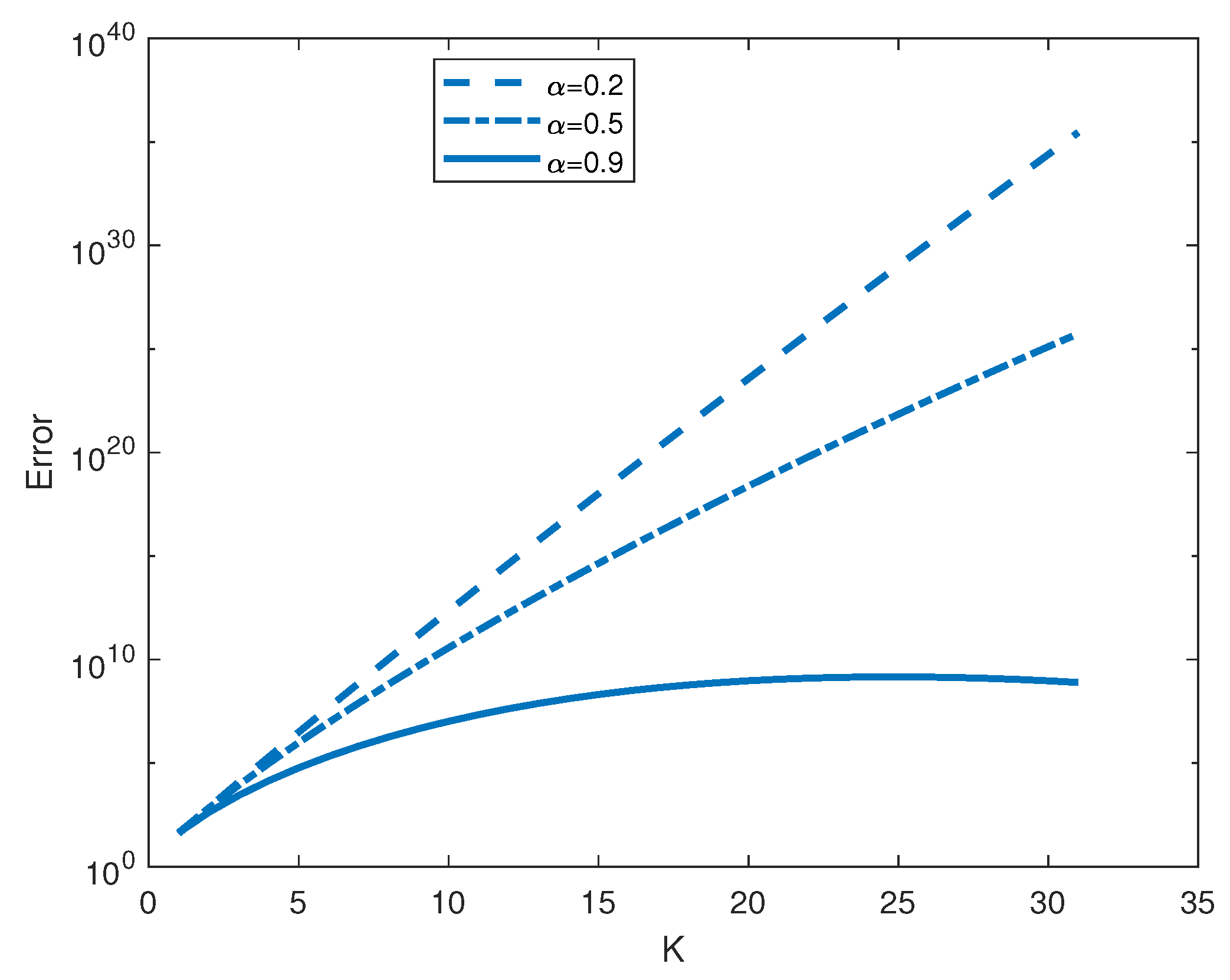
Then, the exact solution can be directly computed as and is the diagonal matrix of diagonal entries and . In Figure 1, we relate the relative error, in norm, between the exact solution and the approximation (5) as K varies, for three different values of and .
Figure 1 clearly shows that the numerical approximation (5) can give unreliable results. In this specific example, the impressive growth of the error is due to numerical cancellation; indeed, the summation terms in Equation (5) get larger as j enlarges and they change sign by passing from the jth power to the next one. This means that we sum up terms with very large modulus and opposite sign, and this is an undisputed source of catastrophic errors.
4.2. Polynomial Methods
Methods based on the minimal polynomial or the eigenpolynomial of a matrix have been proposed to numerically evaluate the matrix ML function. This kind of approach is in general poor and we show the weak points (which are exactly the same we encounter in applying it for the matrix exponential [16]).
The first thing to stress is that they require the eigenvalues’ knowledge. This is usually not a priori available and numerical methods for their computation are usually very expensive. Thus, their application is limited to the case in which eigenvalues are at one’s disposal.
Although in general the minimal polynomial and the eigenpolynomial are very difficult to compute, the latter is simpler to calculate and we focus on this approach.
Let denote the characteristic polynomial of A with
Then, by means of the Cayley–Hamilton theorem, it is easy to prove that any power of A can be expressed as a linear combination of . Thus, also is a polynomial in A with analytic coefficients in t; indeed, formula (2) for the matrix ML function reads
The expression of coefficients is simply obtained once the coefficients are known. However, the weak point is related to their numerical computation since it is very prone to round off error (as shown in [16] already for the 1-by-1 case). For this reason, methods of this kind are strongly discouraged.
4.3. The Schur–Parlett Method Combined with the OPC Method
The third property of Proposition 1 suggests looking for a suitable similarity transformation which moves the attention to the matrix function evaluated in a different argument, hopefully simpler to deal with. In particular, among the best conditioned similarity transformations, one can resort to the Schur one. Indeed, it factors a matrix A as
with T upper triangular and Q unitary. Then,
The Schur decomposition is among the best factorization one can consider since its computation is perfectly stable, unlike other decompositions, as the Jordan one that we will describe in the following. For this reason, it is commonly employed for computing matrix functions [27,28]. The actual evaluation of Equation (7) requires the computation of the ML function for a triangular matrix factor. This topic has been properly addressed for general functions by Parlett in 1976 [29], resulting in a cheap method. Unfortunately, Parlett’s recurrence can give inaccurate results when T has close eigenvalues. In 2003, Higham and Davies [19] proposed an improved version of this method: once the Schur decomposition is computed, the matrix T is reordered and blocked according to its eigenvalues resulting in a matrix, say . Specifically, each diagonal block of has “close” eigenvalues and distinct diagonal blocks have “sufficiently distinct” eigenvalues. In this way, Parlett’s recurrence works well even in the presence of closed eigenvalues of T. Just a final reordering is required at the end of the process to recover from .
The evaluation of starts from the evaluation of the ML function of its diagonal blocks, which are still triangular matrices whose eigenvalues are “close”. Let be one of these diagonal blocks and denotes the mean of these eigenvalues. Then, and
with denoting the k-th order derivative of . The powers of M are expected to decay quickly since the eigenvalues of are close. This means that only a few terms of (8), usually less than the dimension of the block , suffice to get a good accuracy.
Evidently, the computation of (8) involves the computation of the derivatives of the scalar ML function, up to an order depending on the eigenvalues’ properties. This issue has been completely addressed in [18], and we refer to it for the details.
In particular, the analysis of the derivatives of the ML function has been facilitated by resorting to the three parameters’ ML function (also known as the Prabhakar function)
since
The Prabhakar function is an important function occurring in the description of many physical models [30,31,32,33,34,35].
In practice, as for the scalar ML function, one could compute the Prabhakar function, or equivalently the ML derivatives, by the Taylor series for small arguments, the asymptotic expansion for large arguments and an integral representation in the remaining cases. In [18], however, to obtain the same accuracy for all arguments, the inverse Laplace transform has been used in all cases to obtain the simple expression
with any suitable contour in the complex plane encompassing at the left the singularities of the integrand. This last issue is quite delicate: indeed, from a theoretical point of view, the contours chosen to define the inverse Laplace transform are all equivalent while they can lead to extremely different results when the numerical evaluation of these integrals comes into play. Then, an accurate analysis is needed to choose the “optimal” contour which guarantees the desired accuracy, minimizes the computational complexity, and results in a simple implementation. The method proposed in [18], grounded on well established analysis [4,5,15], actually fulfills these requirements since the obtained accuracy is in any case close to the machine precision and the computational complexity is very reasonable. The Matlab code ml_matrix.m implements this method and will be used in the following for numerical tests.
4.4. Jordan Canonical Form
The expression of the matrix ML function in terms of its Jordan canonical form, as stated in Equation (3), could be a direct way to numerically evaluate it. However, the true obstacle in using it is the high sensitivity of the Jordan canonical form to numerical errors (in general, “there exists no numerically stable way to compute Jordan canonical forms” [36]).
To give an example, we consider the Matlab code by Matychyn [37], which implements this approach. We restrict the attention to the exponential case (that is, ) to have as reference solution the result of the well-established expm code by Matlab.
We consider the Chebyshev spectral differentiation matrix of dimension 10. Oddly, even for this “simple” function, the relative error is quite high, namely proportional to .
The error source is almost certainly the well-known ill-conditioning of the eigenvector matrix. Indeed, the code ml_matrix gives a relative error proportional to since it does not involve the Jordan canonical form.
Now, we consider as example the test matrix in [36]
as matrix argument; as before, we just consider the simplest case as a significant example.
For small values of , say , the code [37] stops running, since, when computing the Jordan canonical form, Matlab recognizes that the matrix is singular. On the other hand, the code ml_matrix works very well even for tiny values, say equal to the Matlab machine precision.
Analogously, let
be a matrix. For and , the code [37] just reaches an accuracy proportional to , while the code ml_matrix reaches .
From these examples, we can appreciate the high accuracy reached by the code ml_matrix described in Section 4.3. Moreover, its computational cost is lower than the code based on the Jordan canonical form and, far more important, it does not suffer from the eigenvalues’ conditioning.
4.5. Rational Approximations
Among the nineteen methods to approximate the matrix exponential, Moler and van Loan [16] consider the “exact” evaluation of a rational approximation of the exponential function evaluated in the desired matrix argument. This is indeed a very common approach when dealing with more general functions having good rational approximations (see, e.g., [38,39,40]).
Indeed, let and be polynomials of degree and , respectively, such that, for scalar arguments z,
To evaluate the approximation above in the matrix case, we use a partial fraction expansion of the right-hand side above, leading to
in this way, the computation of is trivial while the sum requires the computation of matrix inversions, namely , for .
Once the rational approximation is fixed, the sum (10) can be computed by actually inverting the matrices if A is a small well-conditioned matrix or, if it is large, incomplete factorizations of A can be cheaply applied [40].
For the ML function, the problem is the detection of a suitable rational approximation to use. The Padé and the Chebyshev rational approximation are commonly preferred for the exponential; this choice is mainly due to their good approximation properties, to the fact that they are explicitly known, and the error analysis is well established.
A key feature of the Padé approximation is that it can be used if is not too large. This does not represent a restriction for the exponential function since it is endowed with the fundamental property
it allows for computing the exponential of an arbitrarily small argument to then extend it to the original argument A. In general, m is chosen as a power of two in order to require only the repeated squaring of the matrix argument.
The property above is only valid for the exponential function, meaning that, for the ML function, there is no direct way to extend the local approximation to the global case.
Some years ago, a global Padé approximation to the ML function was proposed [8] working on the whole real semiaxis . In the matrix case, this restricts the applicability to matrix arguments with real positive eigenvalues. Moreover, the computation of the coefficients is arduous; for this reason, small degrees are considered in [8], which lead to quite important errors.
We now describe the Carathéodory–Fejér approximation of the ML function as an effective tool when a rational approximation is needed.
Carathéodory–Fejér Approximation of the ML Function
As concerns the ML function, Trefethen was the first to address the problem of finding rational approximations when and [41]. Later on, the most general case has been deeply analyzed [11] grounding on the Carathéodory–Fejér (CF) theory; this theory is important since it allows for constructing a near best rational approximation of the ML function. In practice, once we fix a given degree , the residues and the poles are found that define the CF approximation of degree of the ML function. Thus,
When dealing with real arguments, the sum can be arranged as to almost halve the number of terms to compute. Moreover, since a small degree usually suffices to give a good approximation, only a few matrix inverses are actually required. Obviously, this approach is meaningful only for matrix arguments whose inversion can be computed in a stable and reliable way.
5. Numerical Computation of for a Given Vector b
In many situations, the interest is in the computation of for a given vector b. Any method described so far can be applied to compute and then multiply it by the vector b. However, when the dimension of the matrix argument A is very large, ad hoc strategies have to be preferred.
The rational approximation (11) is, for example, a good solution; indeed, it reads
and, rather than matrix inversions, the right-hand side requires only solving linear systems. This approach is effective even for small matrix arguments A, in which case direct methods can be applied for the linear systems involved. When the matrix argument is very large, several alternatives are at one’s disposal: iterative methods can be, for example, applied (see [11]) and, when preconditioning is needed, the same preconditioner can be computed just once and then applied to all shifted systems. Incomplete factorizations of A can be used for example as preconditioners for the systems involved (we refer to [40] for a deep description of the approach).
Krylov subspace methods are an effective tool for the numerical approximation of vectors like ; their first application was related to the exponential and then they have been successfully employed for general functions [38,42,43]. In particular, for the ML function, we refer to [11,12]. The idea is to approximate in Krylov subspaces defined as
The matrix A is projected in these spaces as , where is an orthonormal basis of built by applying the Gram–Schmidt procedure with as starting vector and is an unreduced Hessenberg matrix whose entries are the coefficients of the orthonormalization process.
Then,
where denotes the first column of the identity matrix of dimension .
The potency of these techniques is that usually a small dimension m is enough to get a sufficiently accurate approximation; thus, some classical method usually works to compute .
The convergence of Krylov subspace methods can be quite slow when the spectrum of A is large; this phenomenon was primarily studied for the exponential [44] and successively for the ML function [12]. In these cases, the Rational Arnoldi method can be successfully used, with superb results already for the “one-pole case” [12,45,46,47]. The idea of this method, known as Shift and Invert in the context of eigenvalue problems, is to fix a parameter and to approximate in the Krylov subspaces generated by , rather than A and b.
The computational complexity is larger than for standard Krylov subspace methods since the construction of the Krylov subspaces requires computing vectors of the form , that is, solving several linear systems with the same shifted coefficient matrix. However, for suitable shift parameters, the convergence becomes much faster, to thus compensate the additional cost.
We refer to [12] for a comprehensive description of this method applied to the computation of the matrix ML function, together with the numerical tests to show the effectiveness of the approach. Moreover, for completeness, we want to stress that the actual computation of the matrix ML function in [12] was accomplished by combining the Schur–Parlett recurrence and the Matlab code mlf.m by Podlubny and Kacenak [48]. However, this approach cannot handle the derivatives of the ML scalar function; therefore, to treat more general situations, as, for example, matrix arguments with repeated eigenvalues, the approach described in Section 4.3 has to be considered within the implementation.
6. Conclusions
This paper offers an overview of the matrix ML function: the most important theoretical properties are collected to serve as a review and to help in the treatment of this function. Moreover, the existing methods for its numerical computation are presented, by following the plot used by Moler and Van Loan [16] to describe the methods for the numerical computation of the matrix exponential.
From this analysis, we may conclude that the approach based on the combination of the Schur–Parlett method and the OPC method is the most efficient: it is indeed cheap, accurate, and easy to implement.
Funding
This research was funded by the INdAM-GNCS 2019 project “Metodi numerici efficienti per problemi di evoluzione basati su operatori differenziali ed integrali”.
Conflicts of Interest
The author declares no conflict of interest.
Abbreviations
The following abbreviations are used in this manuscript:
| CF | Carathéodory–Fejér |
| FDE | Fractional Differential Equation |
| ML | Mittag–Leffler |
| OPC | Optimal Parabolic Contour |
References
- Gorenflo, R.; Kilbas, A.A.; Mainardi, F.; Rogosin, S. Mittag–Leffler Functions. Theory and Applications; Springer Monographs in Mathematics; Springer: Berlin, Germany, 2014; 420p, pp. xii, 420p. [Google Scholar]
- Gorenflo, R.; Mainardi, F. Fractional calculus: Integral and differential equations of fractional order. In Fractals and Fractional Calculus in Continuum Mechanics (Udine, 1996); Springer: Vienna, Austria, 1997; Volume 378, pp. 223–276. [Google Scholar]
- Mainardi, F.; Mura, A.; Pagnini, G. The M-Wright function in time-fractional diffusion processes: A tutorial survey. Int. J. Differ. Equ. 2010, 2010, 104505. [Google Scholar] [CrossRef]
- Garrappa, R. Numerical evaluation of two and three parameter Mittag-Leffler functions. SIAM J. Numer. Anal. 2015, 53, 1350–1369. [Google Scholar] [CrossRef]
- Garrappa, R.; Popolizio, M. Evaluation of generalized Mittag–Leffler functions on the real line. Adv. Comput. Math. 2013, 39, 205–225. [Google Scholar] [CrossRef]
- Gorenflo, R.; Loutchko, J.; Luchko, Y. Computation of the Mittag-Leffler function Eα,β(z) and its derivative. Fract. Calc. Appl. Anal. 2002, 5, 491–518. [Google Scholar]
- Valério, D.; Tenreiro Machado, J. On the numerical computation of the Mittag–Leffler function. Commun. Nonlinear Sci. Numer. Simul. 2014, 19, 3419–3424. [Google Scholar] [CrossRef]
- Zeng, C.; Chen, Y. Global Padé approximations of the generalized Mittag–Leffler function and its inverse. Fract. Calc. Appl. Anal. 2015, 18, 1492–1506. [Google Scholar] [CrossRef]
- Garrappa, R.; Moret, I.; Popolizio, M. Solving the time-fractional Schrödinger equation by Krylov projection methods. J. Comput. Phys. 2015, 293, 115–134. [Google Scholar] [CrossRef]
- Garrappa, R.; Moret, I.; Popolizio, M. On the time-fractional Schrödinger equation: Theoretical analysis and numerical solution by matrix Mittag-Leffler functions. Comput. Math. Appl. 2017, 74, 977–992. [Google Scholar] [CrossRef]
- Garrappa, R.; Popolizio, M. On the use of matrix functions for fractional partial differential equations. Math. Comput. Simul. 2011, 81, 1045–1056. [Google Scholar] [CrossRef]
- Moret, I.; Novati, P. On the Convergence of Krylov Subspace Methods for Matrix Mittag–Leffler Functions. SIAM J. Numer. Anal. 2011, 49, 2144–2164. [Google Scholar] [CrossRef]
- Popolizio, M. Numerical solution of multiterm fractional differential equations using the matrix Mittag–Leffler functions. Mathematics 2018, 1, 7. [Google Scholar] [CrossRef]
- Rodrigo, M.R. On fractional matrix exponentials and their explicit calculation. J. Differ. Equ. 2016, 261, 4223–4243. [Google Scholar] [CrossRef]
- Weideman, J.A.C.; Trefethen, L.N. Parabolic and hyperbolic contours for computing the Bromwich integral. Math. Comp. 2007, 76, 1341–1356. [Google Scholar] [CrossRef]
- Moler, C.; Van Loan, C. Nineteen dubious ways to compute the exponential of a matrix. SIAM Rev. 1978, 20, 801–836. [Google Scholar] [CrossRef]
- Moler, C.; Van Loan, C. Nineteen dubious ways to compute the exponential of a matrix, twenty-five years later. SIAM Rev. 2003, 45, 3–49. [Google Scholar] [CrossRef]
- Garrappa, R.; Popolizio, M. Computing the matrix Mittag–Leffler function with applications to fractional calculus. J. Sci. Comput. 2018, 77, 129–153. [Google Scholar] [CrossRef]
- Davies, P.I.; Higham, N.J. A Schur-Parlett algorithm for computing matrix functions. SIAM J. Matrix Anal. Appl. 2003, 25, 464–485. [Google Scholar] [CrossRef]
- Mittag-Leffler, M.G. Sopra la funzione Eα(x). Rend. Accad. Lincei 1904, 13, 3–5. [Google Scholar]
- Mittag-Leffler, M.G. Sur la représentation analytique d’une branche uniforme d’une fonction monogène-cinquième note. Acta Math. 1905, 29, 101–181. [Google Scholar] [CrossRef]
- Wiman, A. Ueber den Fundamentalsatz in der Teorie der Funktionen Eα(x). Acta Math. 1905, 29, 191–201. [Google Scholar] [CrossRef]
- Garrappa, R. Numerical Solution of Fractional Differential Equations: A Survey and a Software Tutorial. Mathematics 2018, 6, 16. [Google Scholar] [CrossRef]
- Higham, N.J. Functions of Matrices; Society for Industrial and Applied Mathematics (SIAM): Philadelphia, PA, USA, 2008; 425p, pp. xx, 425p. [Google Scholar]
- Horn, R.; Johnson, C. Topics in Matrix Analysis; Cambridge University Press: Cambridge, UK, 1994. [Google Scholar]
- Sadeghi, A.; Cardoso, J.R. Some notes on properties of the matrix Mittag–Leffler function. Appl. Math. Comput. 2018, 338, 733–738. [Google Scholar] [CrossRef]
- Del Buono, N.; Lopez, L.; Politi, T. Computation of functions of Hamiltonian and skew-symmetric matrices. Math. Comp. Simul. 2008, 79, 1284–1297. [Google Scholar] [CrossRef]
- Politi, T.; Popolizio, M. On stochasticity preserving methods for the computation of the matrix pth root. Math. Comput. Simul. 2015, 110, 53–68. [Google Scholar] [CrossRef]
- Parlett, B.N. A Recurrence Among the Elements of Functions of Triangular Matrices. Linear Algebra Appl. 1976, 14, 117–121. [Google Scholar] [CrossRef]
- Mainardi, F.; Garrappa, R. On complete monotonicity of the Prabhakar function and non-Debye relaxation in dielectrics. J. Comput. Phys. 2015, 293, 70–80. [Google Scholar] [CrossRef]
- Garrappa, R. Grünwald–Letnikov operators for fractional relaxation in Havriliak–Negami models. Commun. Nonlinear Sci. Numer. Simul. 2016, 38, 178–191. [Google Scholar] [CrossRef]
- Garrappa, R.; Mainardi, F.; Maione, G. Models of dielectric relaxation based on completely monotone functions. Fract. Calc. Appl. Anal. 2016, 19, 1105–1160. [Google Scholar] [CrossRef]
- Garra, R.; Garrappa, R. The Prabhakar or three parameter Mittag-Leffler function: Theory and application. Commun. Nonlinear Sci. Numer. Simul. 2018, 56, 314–329. [Google Scholar] [CrossRef]
- Giusti, A.; Colombaro, I. Prabhakar-like fractional viscoelasticity. Commun. Nonlinear Sci. Numer. Simul. 2018, 56, 138–143. [Google Scholar] [CrossRef]
- Colombaro, I.; Garra, R.; Garrappa, R.; Giusti, A.; Mainardi, F.; Polito, F.; Popolizio, M. A practical guide to Prabhakar fractional calculus. 2019; preprint. [Google Scholar]
- Horn, R.; Johnson, C. Matrix Analysis; Cambridge University Press: Cambridge, UK, 1990. [Google Scholar]
- Matychyn, I. Matrix Mittag–Leffler function. In MATLAB Central, File Exchange, File ID: 62790; MathWorks, Inc.: Natick, MA, USA, 2017. [Google Scholar]
- Lopez, L.; Simoncini, V. Analysis of projection methods for rational function approximation to the matrix exponential. SIAM J. Numer. Anal. 2006, 44, 613–635. [Google Scholar] [CrossRef]
- Trefethen, L.N.; Weideman, J.A.C.; Schmelzer, T. Talbot quadratures and rational approximations. BIT 2006, 46, 653–670. [Google Scholar] [CrossRef]
- Bertaccini, D.; Popolizio, M.; Durastante, F. Efficient approximation of functions of some large matrices by partial fraction expansions. Int. J. Comput. Math. 2019, 96, 1799–1817. [Google Scholar] [CrossRef]
- Schmelzer, T.; Trefethen, L.N. Evaluating matrix functions for exponential integrators via Carathéodory-Fejér approximation and contour integrals. Electron. Trans. Numer. Anal. 2007, 29, 1–18. [Google Scholar]
- Saad, Y. Analysis of some Krylov subspace approximations to the matrix exponential operator. SIAM J. Numer. Anal. 1992, 29, 209–228. [Google Scholar] [CrossRef]
- Frommer, A.; Simoncini, V. Matrix Functions. In Mathematics in Industry; Springer: Berlin, Germany, 2008; Volume 13, pp. 275–303. [Google Scholar]
- Hochbruck, M.; Lubich, C. On Krylov subspace approximations to the matrix exponential operator. SIAM J. Numer. Anal. 1997, 34, 1911–1925. [Google Scholar] [CrossRef]
- Moret, I.; Novati, P. RD-Rational Approximations of the Matrix Exponential. BIT Numer. Math. 2004, 44, 595–615. [Google Scholar] [CrossRef]
- Van den Eshof, J.; Hochbruck, M. Preconditioning Lanczos approximations to the matrix exponential. SIAM J. Sci. Comput. 2006, 27, 1438–1457. [Google Scholar] [CrossRef] [Green Version]
- Popolizio, M.; Simoncini, V. Acceleration techniques for approximating the matrix exponential. SIAM J. Matrix Anal. Appl. 2008, 30, 657–683. [Google Scholar] [CrossRef] [Green Version]
- Podlubny, I.; Kacenak, M. The Matlab mlf code. In MATLAB Central File Exchange, 2001–2009. File ID: 8738.2001; MathWorks, Inc.: Natick, MA, USA, 2017. [Google Scholar]

© 2019 by the author. Licensee MDPI, Basel, Switzerland. This article is an open access article distributed under the terms and conditions of the Creative Commons Attribution (CC BY) license (http://creativecommons.org/licenses/by/4.0/).
Share and Cite
MDPI and ACS Style
Popolizio, M. On the Matrix Mittag–Leffler Function: Theoretical Properties and Numerical Computation. Mathematics 2019, 7, 1140. https://doi.org/10.3390/math7121140
AMA Style
Popolizio M. On the Matrix Mittag–Leffler Function: Theoretical Properties and Numerical Computation. Mathematics. 2019; 7(12):1140. https://doi.org/10.3390/math7121140
Chicago/Turabian StylePopolizio, Marina. 2019. "On the Matrix Mittag–Leffler Function: Theoretical Properties and Numerical Computation" Mathematics 7, no. 12: 1140. https://doi.org/10.3390/math7121140
Note that from the first issue of 2016, this journal uses article numbers instead of page numbers. See further details here.