Digital Supply Chain through Dynamic Inventory and Smart Contracts

Department of Business and Management, LUISS University, 00197 Rome, Italy
Mathematics 2019, 7(12), 1235; https://doi.org/10.3390/math7121235
Submission received: 9 November 2019
/
Revised: 6 December 2019
/
Accepted: 7 December 2019
/
Published: 13 December 2019
(This article belongs to the Special Issue Applications of Operational Research and Mathematical Models in Management)
Abstract
:This paper develops a digital supply chain game, modeling marketing and operation interactions between members. The main novelty of the paper concerns a comparison between static and dynamic solutions of the supply chain game achieved when moving from traditional to digital platforms. Therefore, this study proposes centralized and decentralized versions of the game, comparing their solutions under static and dynamic settings. Moreover, it investigates the decentralized supply chain by evaluating two smart contracts: Revenue sharing and wholesale price contracts. In both cases, the firms use an artificial intelligence system to determine the optimal contract parameters. Numerical and qualitative analyses are used for comparing configurations (centralized, decentralized), settings (static, dynamic), and contract schemes (revenue sharing contract, wholesale price contract). The findings identify the conditions under which smart revenue sharing mechanisms are worth applying.
1. Introduction
Despite its recent advent, supply chain (SC) management was deeply investigated in terms of vertical and horizontal relationships, multitude of tactics and strategies, and various objectives, purposes, and targets, mainly based on the maximization of profit or minimization of costs [1]. Although several contributions emphasized the need for implementing SC strategies, research is still needed to identify the best SC structure and the appropriate methodology for its analysis, especially with new technological disruptions like digitalization, Industry 4.0, and blockchains, which are deeply changing operations and supply chain management. From a methodological point of view, the literature applies both static and dynamic methods to investigate the supply chain management relationships.
The static literature involves time-independent features. In each period, the models do not observe the changes in system parameters, and the main characterization involves decisions on customer demand (deterministic and random, endogenous and exogenous), vertical and horizontal competition within supply chains, and no risk involved, risk incurred by only one or few members, or risk shared between the participants [2].
According to the static literature, the general concept of Nash equilibrium applies for determining the optimal solution, allowing firms to maximize a certain payoff. Starting from this general characterization, the literature proposes multitude types of scenarios including cooperative and non-cooperative settings, simultaneous and sequential decision-making (Cournot and Stackelberg games), vertical and horizontal competition, and embracing numerous areas as pricing (Bertrand’s competition) or production (Cournot’s competition).
In contrast, the dynamic literature considers how the supply chain relationships change and evolve over time. Several subjects can be dynamically analyzed, like the word-of-mouth effect, economies of scale, uncertainty, the bull whip effect, and seasonal, fashion, and holiday demand pattern. In this framework, the system changes can occur at any point of time; consequently, the control of actions and the monitoring of strategies need continuous investigation [3]. SCs adjust their decisions over time, resulting in an inter-temporal interaction among supply chain members. Dynamic setting incorporates a carry-over effect. For example, advertising not only affects the current sales, but it also feeds the brand equity, which in turn has an influence on sales [4]. Ref. [5] proposed the application of a dynamic approach to solve the dilemma between short- and long-term coordination. The first application of a differential game was developed by [6]; afterward, a number of contributions surveyed applications in several areas [7,8,9,10,11,12,13,14,15,16,17,18].
As highlighted by [17], although analyzing supply chains in a static framework generates myopic attitudes, in reality, it remains an ideal solution for supply chain coordination under particular conditions. Similarly, some static mechanisms also coordinate the SC in dynamic settings, whereas others do not [19]. This research contributes the described framework in which the effectiveness of static and dynamic approaches for supply chain coordination is not clear and the boundaries of applications are not clearly defined. According to the literature, several coordination schemes exist. Each of them possesses particular characteristics, and their adoption depends on both the SC structures and the inter-temporal setting. Previous literature showed numerous contributions identifying various contract schemes for supply chain coordination as sales rebates [20], buy-back [21], quantity flexibility [22], quantity premium contract [23], wholesale price and revenue sharing contract [21], and quality targets [16].
To provide both theoretical and practical evidence, this research compares the results of two smart contracts, that is, wholesale price (WPC) and revenue sharing contracts (RSC) in both static and dynamic settings. Accordingly, we are able to highlight both the advantages and the disadvantages of each approach to achieve supply chain coordination [24]. Only few contributions studied the differences between static and dynamic frameworks, as well as their limits and applications [2,25]. Moreover, according to [21], wholesale price and revenue sharing contracts generate different and controversial results depending on the SC structure. By setting a static framework, the authors showed that a revenue sharing coordinates a supply chain including one supplier and one retailer, while it fails in the case of multiple retailers and, consequently, WPC is preferable. Each player prefers RSC with respect to WPC whenever the revenues shared exceed the revenues lost due to a lower transferring price. Nevertheless, RSC is difficult to administer and extremely costly; the contract designer could prefer the implementation of a simple and traditional contract coordinating the SC even when it generates some negative externalities.
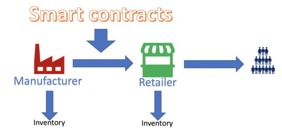
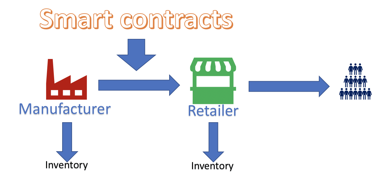
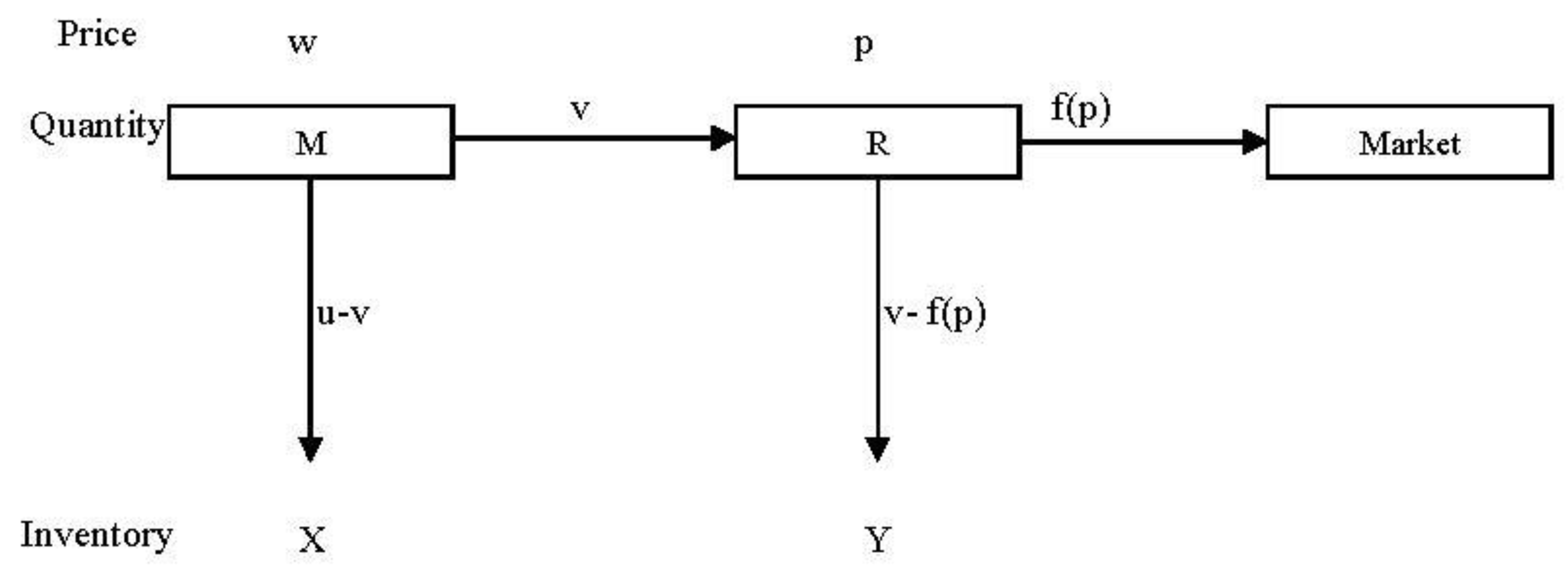
This research extends the study by [21] by proposing a dynamic version of their model and including the digitalization of the supply chain [24]. The findings take position in the literature by comparing RSC and WPC inside static and dynamic frameworks. Figure 1 reports the adopted SC structure which appeared in [6] and, more recently, in [19].
The SC structure consists of one manufacturer (firm he) and one retailer (firm she). The manufacturer makes the quantity u and sells the quantity v to the retailer at a price w. The difference between these two quantities represents his inventory X. The retailer purchases v and sells f(p) to the market. f(p) = a − bp represents the inverse demand function adopted by [6,26], where a and b are positive constants. The difference between v and f(p) is the retailer’s inventory Y.
The retailer fixes the price while the wholesale price is exogenous and intended as determined by an artificial intelligence system that supports the decision-making process. Under RSC, both players share some revenue through the parameter and determine the transferring price w0 such that w0 < w. Firms can use artificial intelligence to identify the best parameters for maximizing their profit functions [27], complementing the system with other technologies like blockchain and big data. Therefore, the contracts become smart contracts.
Beyond presenting and comparing several decentralized SCs characterized by the adoption of WPC and RSC under static and dynamic frameworks, this research proposes the centralized solution, which is one main element of a digital supply chain. Industry 4.0 technologies allow firms to be fully integrated, and the centralized solution is the best formulation representing this framework. In fact, the artificial intelligence identifies the best contract terms according to the best possible outcomes of a supply chain, which is clearly given by the centralized solution. Hence, the centralized SC is a benchmark [27].
This research is organized as follows: Section 2 describes the differences between static and dynamic games. Section 3 introduces the static formulation of the game proposing both centralized and decentralized solutions. Section 4 develops the dynamic version of the theoretical game following the same steps of Section 3, i.e., centralized and decentralized solutions first and their qualitative comparison afterward. Section 5 proposes numerical analysis of the models developed in Section 2 and Section 3, while the last section concludes and presents future directions.
2. Technical Differences between Static and Dynamic Games
The existing literature on inter-firm relationships reports extensively on a large number of theoretical games using both static and dynamic modeling. Essentially, the choice of their adoption depends on the nature of the game. On one hand, static models are time-independent. Any change in the parameters of the system is completely ignored, thereby generating myopic solutions [25]. This class of game is mainly used to characterize decisions on customer demand (deterministic and random, endogenous and exogenous), vertical and horizontal competition, and no-risk actions [21]. On the other hand, a dynamic setting appears to be considerably more appropriate when modeling variables characterized by carry-over effects. For instance, advertising not only affects current sales considerably, but it also feeds the brand equity, which in turn has an influence on sales [28]. Other diffused examples are represented by the “word-of-mouth” effect, economies of scale, uncertainty, the “bull whip” effect, and seasonal, fashion, and holiday demand patterns [21]. In these frameworks, changes may occur at any point in time; consequently, the control of actions is investigated continuously [15].
A static game involves players choosing several strategies simultaneously (one-shot game) or sequentially (strategies are chosen when needed). The static game is cooperative as the players make side-payments or form coalitions [21]. Nash formulates the solution for a non-cooperative game, in which each player maximizes his own objective or payoff function.
A pair of strategies u1 and u2 is a Nash equilibrium (NE) if, for every and , the following pair of inequalities holds:
No players can do better or get more by choosing an action different from ui*, and no player has incentives for choosing any other strategy. In particular, the Nash solution becomes
If the problem is static, strategy sets are not constrained, and the payoff functions are continuously differentiable [21]. First-order conditions apply for finding the best response functions. The NE needs the resolution of a system of best responses translated into a system of first order (necessary) in optimal conditions.
Moreover, the payoffs are maximized when the second-order condition of (sufficient) optimality holds:
The NE uses the concept of best response for finding the solution of the game and for maximizing the players’ payoffs. Each player chooses the best available action, which generally depends on the other players’ actions. In this sense, whenever a player chooses his own actions, he should have in mind the possible actions that the other players might choose (belief). Consequently, the Nash solution changes to
Optimal conditions change accordingly. For further information on the static approach, see the studies by [21,29].
Similarly, dynamic games or differential games involve at least two players having different objective functions. The existing models embrace non-cooperative and cooperative games; however, in both cases, players’ interrelationships and coordination change over time. Both players select the values of their control and state variables, and the game varies according to one or more differential equations. In the case of a two-player game (i = 1, 2), player 1 chooses his control variable, u1, in order to maximize
while player 2 maximizes
with both maximization problems subject to the following state equations:
The standard problem assumes the controls to be continuous piecewise, while are both known and continuous differentiable functions in the four arguments.
Starting from this general formulation, various researches developed the concept of NE in a dynamic setting, occurring whenever
where and describe the optimal control variables of the players. Two mainstream strategies are applied in differential games: Open and closed (feedback) strategies. In the open-loop strategies, each player selects the values of his control variable at the outset of the game, the instantaneous value of which is only a function of time. Players commit their actions at the beginning of the game without making any modification; they do not update the game according to the available information [15].
Hamiltonian and necessary conditions for optimality easily allow the determination of the NE open-loop strategy. For i = 1, 2 and j = 1, 2, the standard optimal control analysis involves
In reality, players commit to the entire course of actions over time, revising their actions as the game instantaneously evolves, according to the state of the system. This class of strategies coincides with the closed-loop strategies.
The instantaneous control is a function not only of time but also of the state of the system x1(t), x2(t) at that time. In this sense, the closed-loop strategy result is a perfect subgame. The game continues at a new stage representing a subgame of the original one. The state of the system variables evolves accordingly to the new state. A feedback strategy allows the players to take their best decisions even if the initial state of the subgame evolves under suboptimal actions, revealing optimality for the initial game, as well as for every subgame evolving from it.
Previous studies did not apply that class of strategy as frequently as the open-loop strategy. Numerous computational difficulties exist. Even when applying Hamiltonian and first-order conditions, the closed-loop games require the computation of the other players’ feedback strategy. For i = 1, 2 and j = 1, 2, the feedback strategy requires the following conditions:
The second part of the right-hand side of the co-states identifies the interaction term. It also requires the computation of partial differential equations; hence, the optimal solution is not guaranteed. Finding player 1′s optimal feedback strategy requires knowing players 2′s optimal feedback strategy, which requires knowing player 1′s feedback strategy, and so on. However, the closed-loop strategy describes the real competition and the firms’ interactions more appropriately. For further information on the dynamic approach, see the studies by [21].
When players adopt the optimal open-loop concept, they design the optimal strategy at the beginning of the planning horizon and then stick to it until the end. By contrast, the term “memoryless” characterizes closed-loop strategies that change over time as new information becomes available [25].
Table 1 summarizes the main differences between static and dynamic games. Static games mainly apply for single (one-shot) games. Their application to the supply chain (SC) does not seem appropriate since long-term and cooperative relationships characterize those games. Nevertheless, the literature shows numerous studies applying static games to short-term and single-period relationships and reporting myopic solutions. In static games, the optimal value of the players’ decision variables is derived by developing a system of first-order conditions. Time does not influence any of them. Static games use the concept of best response for finding the most favorable outcomes for the players, taking other players’ strategies as given [21]. They search for the NE, that is, the point at which each player selects his best response with respect to the other players’ strategies in order to maximize his payoff.
Dynamic modeling fits adequately when modeling long-term inter-firm games. By choosing the optimal control variables, dynamic modeling describes the optimal trajectory of the state variables that optimizes the players’ objective functions. Differential games adequately model cooperative and non-cooperative settings. Each rule is defined from the beginning of the game, and players keep or modify it according to the adoption of an open- or a closed-loop strategy. An open-loop strategy, in fact, definitely fits when modeling integrated SCs that are characterized by diffused trust, collaboration, and commitment. A closed-loop strategy, in contrast, models SCs that are not at all integrated, as well as partnerships, alliances, and other forms of inter-firm relationships, in which the partners develop long-term strategies that are mainly driven by coordination [19].
Static and dynamic methods are extensively applied to firm games, modeling cooperative and non-cooperative scenarios. They cover several areas and show theoretical and practical results. The next section introduces the state of the art in static and dynamic games with particular attention to SC games. This class of game, in fact, received significant attention recently, while monopolist and oligopolistic scenarios rarely appear in today’s world of business.
3. Characterization of the Static Game
In the formulation of the static model, the manufacturer and retailer maximize their own profit functions, and , respectively. We refer to this model as an SC game, because the two firms compete with each other in the maximization of their profits. Therefore, each firm sets the optimal strategies to maximize its own profit function rather than maximizing the profit function of the entire chain. Equations (1) and (2) illustrate these functions.
The retailer benefits from total revenue that is shared with the manufacturer depending on the contract scheme adopted. According to Equations (1) and (2), the parameter describes the sharing of revenues between the two players under RSC that is determined by an artificial intelligence system that supports the firms’ contractual development. In this latter case, the sharing parameter shows values comprised in the interval (0, 1). As its value increases, the amount of revenue transferred from the retailer to the manufacturer decreases. In contrast, as its value approaches 0, the revenue shared with the manufacturer increases. = 1 reflects the wholesale price scheme, in which the manufacturer does not obtain any share of the retailer’s revenue.
This research adopts similar production and purchasing functions as those introduced by [26]. In particular, the manufacturer’s production and the retailer’s purchasing cost functions take a quadratic form, and , respectively. represents the marginal production (purchasing) cost, while the total cost has a quadratic form; as the quantity produced (purchased) increases, the total production (purchasing) cost decreases. represents the optimal production (purchasing) quantity for exploiting economies of scale and minimizing the total production (purchasing) costs. The convexity of the quadratic cost function imposes penalties when u and v diverge from the target level and .
The last part of the profit functions concerns the holding inventory costs. and are the manufacturer’s and retailer’s marginal inventory costs, while expressions and represent the quantities held in stock by the manufacturer and the retailer, respectively. The manufacturer’s stock includes the initial quantity , the production rate u, and the retailer’s purchasing rate v. The retailer’s stock accounts for the initial quantity , the purchasing rate , and the quantity sold .
As long as this research characterizes the static game, it presents the existence of the NE as a solution of the previous system. It is assumed that the manufacturer entirely satisfies the quantity demanded by the retailer and, similarly, the retailer entirely satisfies the demand by the market; hence, u > v > f(p). Assuming that the transferring price w is given and exogenous, u denotes the manufacturer’s decision variable, while v and p indicate the retailer’s one. The NE is a pair of strategies , such that neither the manufacturer nor the retailer deviate.
In particular:
The existence of the Nash equilibrium is checked through verifying the concavity of the player’s payoff. Suppose that the strategy space is compact and convex, and the payoff function is continuous and quasi-concave with respect to each player’s strategy. There exists at least one Nash equilibrium in pure strategy. Easily, the quasi-concavity of the profit functions applies for both players. Given a parameter such that , concavity is generally given by
Proposition 1.
Quasi-concavity of the profit function is a necessary condition for optimality.
Proof.
Since the quasi-concavity is expressed by
the necessary condition for optimality in Equation (5) holds. For each 0 < < 1, the linear combination of one pair of profit functions is always lower than the maximum profit generated by one of the two strategies. □
As proposed by [1], we may use the implicit function theorem for investigating the uniqueness of the equilibrium.
Proposition 2.
The equilibrium of the game is unique with respect to the production and purchasing rate.
Proof.
is zero for both players since the variables at the denominator are independent, while the absolute value of is higher than zero; therefore, the resulting equilibrium exists and is unique. □
3.1. Centralized Solution of the Static SC Game
When studying the centralized SC, the original objective functions in Equations (1) and (2) sum up in a unique one. The game becomes a Pareto static game [30]. Several contributions introduced the profit function in centralized SC. [2] introduced the centralized SC composed by one supplier and one manufacturer, showing decentralized and centralized profit functions in RSC in a static game. [25] proposed centralized and decentralized profit functions in static and dynamic settings for Stalkeberg and Cournot games. To get the centralized profit function, the firms’ profit functions in Equations (1) and (2) are summed up, implying the elimination of the transferring value . Finally, the centralized SC profit function results.
In the centralized formulation of the static model, the firms behave as one player working as a single entity. The first order condition for the decision variables is as follows:
Substituting Equations (9)–(11) into Equation (8), the profit function in centralized SC becomes
Equation (12) is the benchmark of the SC game under static settings. Whatever the coordination scheme adopted under decentralized settings, Equation (12) shows always higher profits.
The centralized solution is a positive benchmark since it allows firms to identify the best outcomes that they can get. The artificial intelligence system uses the centralized solution to search for the best contract terms to be used in supply chain coordination.
3.2. Decentralized Solution of the Static SC Game
In order to characterize the equilibrium with respect to the manufacturer’s and retailer’s decision variables and finding the solution of the decentralized SC, this research develops the necessary conditions for optimality of both Equation (1) and Equation (2).
The parameter plays a key role in determining the price inside the two different schemes.
Lemma 1.
By adopting WPC in the WPC scheme, since , the selling price results higher than that of RSC.
Since, in RSC < 1, this regime is characterized by a price lower than the wholesale price contract, [31,21] described Equation (16) by investigating the advantages and disadvantages of the two coordination contracts, whereby RSC mitigates the double marginalization effect.
Since the parameter does not exist in Equations (13) and (14), the quantities produced and sold in RSC and WPC are equal. Moreover, while Equation (13) remains always identical independent of the contract scheme, Equation (14) changes with respect to the transferring price w. In the WPC, in fact, the transferring price w0 is higher than that of RSC. The manufacturer reduces the transferring price from w0 to w whenever the revenue received from the retailer compensates for the decreasing wholesale price. Similarly, the retailer accepts the RSC if and only if the economic benefits due to a lower transferring price overcome the lower revenue. In sum, the players shift from WPC to RSC whenever
Upon introducing the sharing parameter and adjusting the transferring price, the players’ strategies change. The manufacturer decides the producing quantity and reduces the transferring price, whereas the retailer purchases higher quantities at a lower price and shares revenues with the manufacturer. According to Equation (17), adopting RSC, both players result economically better off.
Lemma 2.
In WPC, the transferring price is higher than that of RSC, and this generates differences in the quantity purchased.
The difference in the quantity purchased depends on the difference in the transferring prices.
Substituting Equations (13)–(15) into Equations (1) and (2), we obtain the firms’ profit functions in static settings.
Proposition 3.
Under the static setting, RSC is more profitable than WPC for both M and R.
Proof.
Proposition 3 holds because of Lemmas 1 and 2. In RSC, the lower transferring price and the higher quantity purchased generate higher total profits than those under a WPC. According to [19], RSC mitigates the double marginalization effect and makes the players economically better off. □
3.3. Comparison between Centralized and Decentralized Solution of the Static SC Game
This section compares the qualitative solutions of centralized and decentralized configurations in terms of profit. Since the RSC generates higher profit than WPC, the relationships between the profits of centralized and decentralized SCs finally result as follows:
In the static formulation of the game, the centralized SC generates higher profit than the decentralized one in the RSC scheme, while the decentralized SC in WPC always generates lower profits compared to those of the previous scenarios. Among all possible sharing parameter values, artificial intelligence suggests adopting a sharing parameter that makes all firms economically better off. Interestingly, the artificial intelligence embedded in blockchains does not allow firms to reach the same outcomes of the centralized solution. In particular, the condition under which the centralized setting produces higher profits than RSC is . This condition highlights the importance of the parameter chosen by artificial intelligence for comparing the two settings. makes the RSC setting more convenient than the centralized one and, ceteris paribus, the previous condition does not hold. Considering , the players do not take advantages from a centralized SC and, moreover, the decentralized SC results more profitable. Nevertheless, considering the parameter , that is, hypothesizing a WPC scheme, the convenience in implementing a centralized SC depends on the condition . Whenever this latter condition holds, in fact, the centralized setting always makes a higher profit than the decentralized one. If , the profits under centralized SC and WPC are equal. Moreover, this is true when . Whenever this difference is small enough, the previous condition becomes ; hence, the centralized setting is not suitable whenever . Therefore, the artificial intelligence and the blockchain system should be created to use big data with the idea of achieving this shared target to make the supply chain better off from an economic and an operational point of view.
This paper extends the analysis of the game not only to the Nash solution but also to the Stackelberg one. This extension has the purpose of highlighting the convenience of playing either Nash or Stackelberg for improving the players’ results as much as possible. Nevertheless, the structure of the game does not allow playing the Stackelberg game. When the manufacturer is the leader, the game does not change at all with respect to the Nash solutions. The manufacturer’s decision variable, in fact, is u. As the Stackelberg game requires the integration of the leader’s announced strategy inside the retailer’s objective function, the game remains completely the same. The retailer’s strategy is not influenced by the manufacturer’s decisions. When the retailer is the leader of the game, again, the solution is not interesting at all. The retailer’s decision variables are v and p, and both of them should be replaced inside the manufacturer’s strategy. Nevertheless, neither v nor p influence the manufacturer’s choices; thus, the Stackelberg game is not interesting as it coincides with the Nash solution. This result derives from the lack of interferences between the players’ decision variables. The structure of the game matters when facing the comparison between Nash and Stackelberg games and should be adequately defined when the comparison is the aim of the study. In all these cases, the artificial intelligence system is not able to find an adequate contractual term to propose. The blockchain does not find a visible solution, and the miners are not able to solve the problem because the solution is equivalent to the previous one.
4. Characterization of the Dynamic Game
As for the static model proposed in Section 2, the purpose of the dynamic model is to maximize the firms’ profit functions, and . The differential game has the same structure as the static one; this similarity allows us to compare them appropriately. Also, in dynamic settings, in fact, the retailer decides the market price and purchased quantity given by p and v, respectively, while the manufacturer decides the production rate, u. The total revenue [a − b(p)] p is shared with respect to the parameter as the players adopt the RSC scheme. The artificial intelligence system is always in charge of deciding the optimal ranges for the sharing parameter. In fact, implies SC coordination through the WPC. The wholesale price and the sharing parameter are also determined by the blockchain, where the miners are asked to solve a more complicated algorithm, which is linked to the dynamics behind the differential games, whose outcomes would eventually lead to smart contracts.
In addition to the previous formulations, we introduce a digitalization option made through information sharing on inventory at all SC levels. This is realized through the adoption of Industry 4.0 technologies in the supply chain [24]. For describing the cost functions, the considerations made for the static game are still valid. The holding cost functions are assumed linear into the objective functions since their motions are controlled by [21] state equations.
By using these two state equations, this research investigates how players’ stocks vary over time. In particular, Equation (23) represents the manufacturer’s state equation, and shows how stocks are controlled over time by the manufacturer’s production rate, u, and by the retailer’s purchasing rate, v. Equation (24) is the retailer’s state equation, which controls the retailer’s stocks over time by the purchasing rate, v, and by the inverse demand function, .
The firm’s profit functions are as follows:
Since a short planning horizon is hypothesized, the discounting factor is not considered in our analysis.
4.1. Centralized Solution of the Dynamic SC Game
As for the static model, this paper presents the centralized dynamic model. This latter model produces a Pareto dynamic optimal solution, since both players make the highest possible profits. Whatever the coordination scheme adopted, the total profits generated are always lower or at least equal to the Pareto dynamic solution, which represents the benchmark of the game. Dynamic centralized settings were extensively proposed recently [27]. In this paper, the authors highlighted the benefits of collaboration in decentralized settings. In this paper, the artificial intelligence working in blockchains uses the centralized solution as a benchmark, searching for a sharing parameter that dynamically optimizes the firms’ profits.
The centralized dynamic model is derived by summing up Equations (25) and (26). Since the players behave as a unique entity, the sharing parameter and the transferring price disappear.
Also, in centralized settings, the discount factor is not considered since the time horizon is assumed to be short enough. By using Equations (23) and (24), the related Hamiltonian results as follows:
where and are the co-state variables. Beyond including the state Equations (23) and (24), this problem considers the following constraints: At any instance of time, the feasible controls u and v take non-negative values and the state constraints X > 0 and Y > 0 must be satisfied. Following this constraint, the necessary optimal conditions are derived for u, v, and p as follows:
By using Equation (29) and the transversality condition in Equation (30), it is easy to show that < 0 for . reflects the implicit value of the inventory X(t), and its negative value shows inefficiency in retaining or marginally increasing the stocks. This result is a consequence of the assumption X > 0. Centralized SC has no incentive to increase inventory. Equation (29) represents the optimal necessary condition for implementing an efficient producing policy in centralized SC. By differentiating and by using the relative transversality condition , it follows that . Moreover, and This latter expression indicates that the centralized SC does not reach the optimal efficient level of production at the end of the planning horizon. represents the loss of efficiency as the salvage value is negative.
Similarly, by using Equation (31) and the transversality condition in Equation (32), as it is assumed that Y > 0, < 0 for . reflects the implicit value of the inventory Y(t), and its negative value shows inefficiency in retaining or marginally increasing stocks. Also, the centralized SC has no incentive to increase inventory. Equation (31) represents the optimal necessary condition for implementing an efficient purchasing policy under centralized SC. By differentiating and by using the relative transversality condition , it follows that . As and , the centralized SC misses the optimal efficient level of purchasing at the end of the planning horizon. represents the loss of efficiency as the salvage value is negative.
From Equation (33), the price policy in centralized SC shows two critical elements values; > 0 indicates the maximum market price, while is the marginal convenience in keeping stocks; hence, it has negative value.
In the centralized SC, the parameter disappears completely. The two players behave as a unique entity, taking advantage of centralization, while also eliminating the double marginalization effect. The transferring price is equal to the marginal producing cost. We use Equations (29), (31), and (33) to resolve the state equation in centralized SC.
By manipulating Equations (34) and (35) and differentiating the state equations with respect to time, we obtain the following system:
Substituting the values from Equations (29), (31), (33), (36), and (37) into Equation (27), the centralized SC profit function in dynamic settings is as follows:
4.2. Decentralized Solution of the Dynamic SC Game
In order to characterize the decentralized solution of the dynamic SC game, this session develops the Hamiltonian for both players showing necessary and sufficient conditions for optimality. The manufacturer’s problem for determining the optimality conditions is as follows:
where and are the co-state variables. The manufacturer’s problem includes the two state Equations (23) and (24) and the following constraints: At any instant of time, the feasible control u takes non-negative values and the state constraints X > 0, Y > 0 must be satisfied.
The necessary optimality conditions are as follows:
Because of the linearity of the game, the condition in Equation (40) is sufficient for optimality. Using Equation (41), we can show for . Therefore, from Equation (40) and the transversality condition in Equation (41), it follows that holds for , and . reflects the manufacturer’s marginal inventory cost and influences the value of X. Since it is negative, the manufacturer has no incentive to marginally increase stocks. reflects the economies of scale in production; as u approaches , the production cost decreases. implies that the manufacturer does not influence the retailer’s inventory policy.
The Hamiltonian maximization condition in Equation (41) shows that the marginal production cost is equal to the marginal inventory cost. Equation (40) represents the manufacturers optimal production policy. By differentiating Equation (41) and by using the transversality condition in Equation (21), it results that
Finally, the condition holds for , and ; therefore, the optimal production rate is given by
Similarly, the retailer’s optimal control problem consists of determining the optimality conditions for v and p, which are the purchasing rate and market price, respectively.
where and are the retailer’s co-state variables.
The retailer’s problem includes the two state Equations (23) and (24) and the following constraints: At any instant of time, the feasible control v and p take non-negative values and the state constraints X > 0, Y > 0 must be satisfied.
Since we modeled a linear game, open- and closed-loop solutions coincide. The equilibrium degenerates at a closed-loop solution depending only on time; the final result is a sub-perfect Nash equilibrium, and the solution is Pareto optimal. Necessary optimality conditions for v and p are as follows:
Equation (47) implies that the retailer does not influence the manufacturer’s inventory policy. Equation (47) shows that for , and, from Equation (21), it follows that for holds. reflects the retailer’s marginal inventory cost and, implicitly, the value of Y. Negativity of this value implies that the retailer has no incentive to marginally increase stocks, according to the assumption Y > 0.
Equation (45) represents the retailer’s optimal purchasing policy. By differentiating Equation (46), it results that
Therefore, for and . At the end of the planning horizon, the optimal retailer’s quantity is given by
Equation (24) represents the necessary condition with respect to the price. In the retailer’s price strategy, two elements appear; the first is > 0, which indicates the maximum market price, and is strictly positive, while the second term is the retailer’s marginal convenience in holding stocks, and its value is negative.
From this result, the main intuition concerns the double marginalization effect deriving from the transferring price and the marginal processing cost. According to [31], the double marginalization effect disappears as the transferring price is equal to the marginal production cost; all coordination contracts also contain, among others, this condition. Previous studies introduced several coordination schemes. Also, in the dynamic framework, the RSC mitigates the double marginalization effect. Since it contains theoretical and practical advantages and disadvantages, its results are compared with the WPC, essentially based on a fixed transferring price charged without considering any players’ agreements, concerning neither revenue sharing nor price discounts. In particular, Equations (25) and (26) are structured in the RSC framework since the retailer shares some revenue defined by the parameter .
Lemma 3.
By adopting the WPC scheme in a dynamic framework, the selling price is higher than that of RSC.
Inside the dynamic setting, the selling price increases over time, while both prices are equal at the end of the planning horizon.
Since T > t, (T − t) is always decreasing and the price increases over time . The lower is, the lower the price is. At the beginning of the planning horizon, ; since T > t, the selling price increases over time for and converges to at the end of the planning horizon.
Nevertheless, the sharing parameter does not enter Equations (45) and (40); hence, the quantity produced and sold under RSC and WPC is identical. However, while Equation (40) is totally independent of the contract scheme since the transferring price does not appear, the difference in the transferring prices in the two contract schemes also generates a difference in the retailer’s purchasing policy. In particular, the quantity purchased in WPC is lower than that of RSC, resulting in the following equation:
Since the transferring price does not enter Equation (40), similarly to the static game, the manufacturer does not modify its producing policy depending on the contract scheme. In contrast, the retailer changes his purchasing policy according to the difference between w and w0. When coordinating the SC by RSC, the quantity purchased is higher. As the gap between transferring price increases, so does the distance between WPC and RSC quantities.
We can state the sufficient optimality conditions in terms of the Hamiltonian by using the Arrow approach. Consider the Hessian matrix for both players consisting of the four partial derivatives of the maximized Hamiltonian with respect to X and Y.
Proposition 4.
The necessary conditions for optimality are also sufficient.
Proof.
In the matrix in Equation (32), the off-diagonal elements are zero. Using the rule of principal minors, we conclude that, for both players, the maximized Hamiltonian is concave in (X, Y); hence, the necessary conditions for optimality are also sufficient. □
We use the results from Equations (40), (45), and (48) to resolve the state equations.
By adequately manipulating Equations (55) and (56) and differentiating the state equations with respect to time, the solution of the previous system is as follows:
Substituting the values from Equations (40), (45), (48), (57), and (58) into Equations (25) and (26), the firms’ profit functions in dynamic settings are as follows:
Proposition 5.
Under the static setting, RSC is more profitable than WPC for both firms.
Proof.
Proposition 6 holds because of Lemma 3 and Lemma 4. In RSC, the lower transferring price and the higher quantity purchased generate higher total profits than those of WPC in a dynamic setting. RSC mitigates the double marginalization effect and makes the players economically better off. □
4.3. Comparison between Centralized and Decentralized Solutions of the Dynamic SC Game
The previous equation fixes an economic benchmark in the dynamic setting. Independent of the coordination scheme adopted, the total SC profits do not exceed that benchmark. According to Proposition 6, the RSC scheme generates higher profits than WPC, and knowing the Pareto solution produces generally higher results, the comparison between dynamic schemes results in the following equation:
Centralized SC generates higher profits as compared to decentralized solutions coordinated by RSC or WPC. This is true when
These expressions represent centralized SC and decentralized SC under RSC and WPC in dynamic settings. The left-hand side of the expression shows the convenience of centralizing the SC expressed in terms of lower costs as compared with the RSC and WPC solutions reported in the middle and right-hand sides of the expression, respectively. The sharing parameter and the difference between and w make the various settings different. As , RSC and WPC generate the same profits, and the players agree on centralizing the SC when . This is also true whenever . As , centralized and decentralized SCs under WPC generate the same results, and Equation (61) does not hold since the RSC produces lower profits. When the manufacturer is indifferent with respect to producing and keeping stocks. He is not advantaged upon coordinating the SC; therefore, the simple WPC is preferable. When , centralization makes the players better off with respect to non-centralized solution; the manufacturer’s inventory cost is in fact lower; hence, centralization produces efficiency in the higher part of the SC. By resolving the left-hand and middle parts of Equation (62), and by integrating and simply manipulating the equations, the threshold of the sharing parameter in dynamic setting results in the following equation:
with
As for the static setting, the dynamic development of the game does not consider the Stackelberg solution. This choice derives from the same motivations expressed previously. When assuming the manufacturer is the leader, upon announcing his decisions at first, the value of the decision variable u should be replaced inside the retailer’s profit function in Equation (40), and then deriving the optimal conditions. As v and p are the retailer’s decisions variables, the players’ problems do not change. When assuming the retailer is the leader, upon announcing his strategy at first, the values of p and v should be replaced inside the manufacturer’s profit function in Equation (25). Even in this case, the manufacturer’s strategy does not change as p and v do not interfere with u. The decisions of each player are not influenced by the others’ strategies; hence, the Stackelberg game does not provide more information than the Nash game. Once again, this result comes from the structure of the game. As our purpose is to compare the economical convenience in adopting alternative coordination schemes under static and dynamic settings, the next section develops the numerical analysis.
5. Numerical Analysis
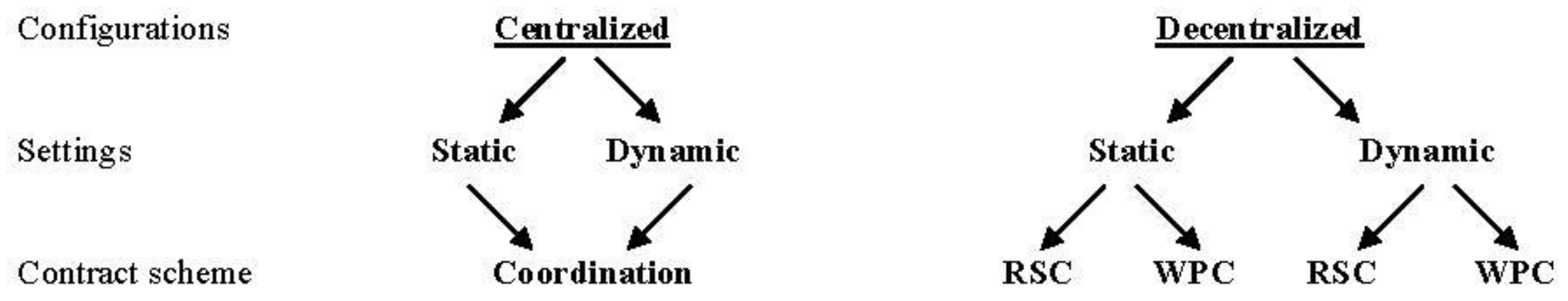
Figure 2 summarizes all possible configurations derived previously considering two contract schemes (RSC and WPC), two settings (static and dynamic), and two configurations (centralized and decentralized SC).
In order to introduce a sound comparison between the previous models and then confirm and/or disconfirm existing results in the literature, we set up numerical analysis following the current trend of research in supply chain management using simulation models in this framework. Table 2 reports the base parameter values used.
With this setting, this study made the following assumptions:
- The marginal production and purchasing costs, as well as the inventory costs, are the same; therefore, each player is indifferent with respect to producing or holding stocks.
- Nevertheless, by producing and purchasing, each player can reach the optimal production and purchasing quantity. This represents the optimal amount of goods to attain in order to exploit the economies of scale and minimizing the total production and purchasing costs. Also, those quantities are assumed equal for both players.
- The transferring price under RSC is equal to the production cost. The manufacturer does not increase his profit directly by selling but receives a compensating quota of the retailer’s income. The parameter describes that proportion.
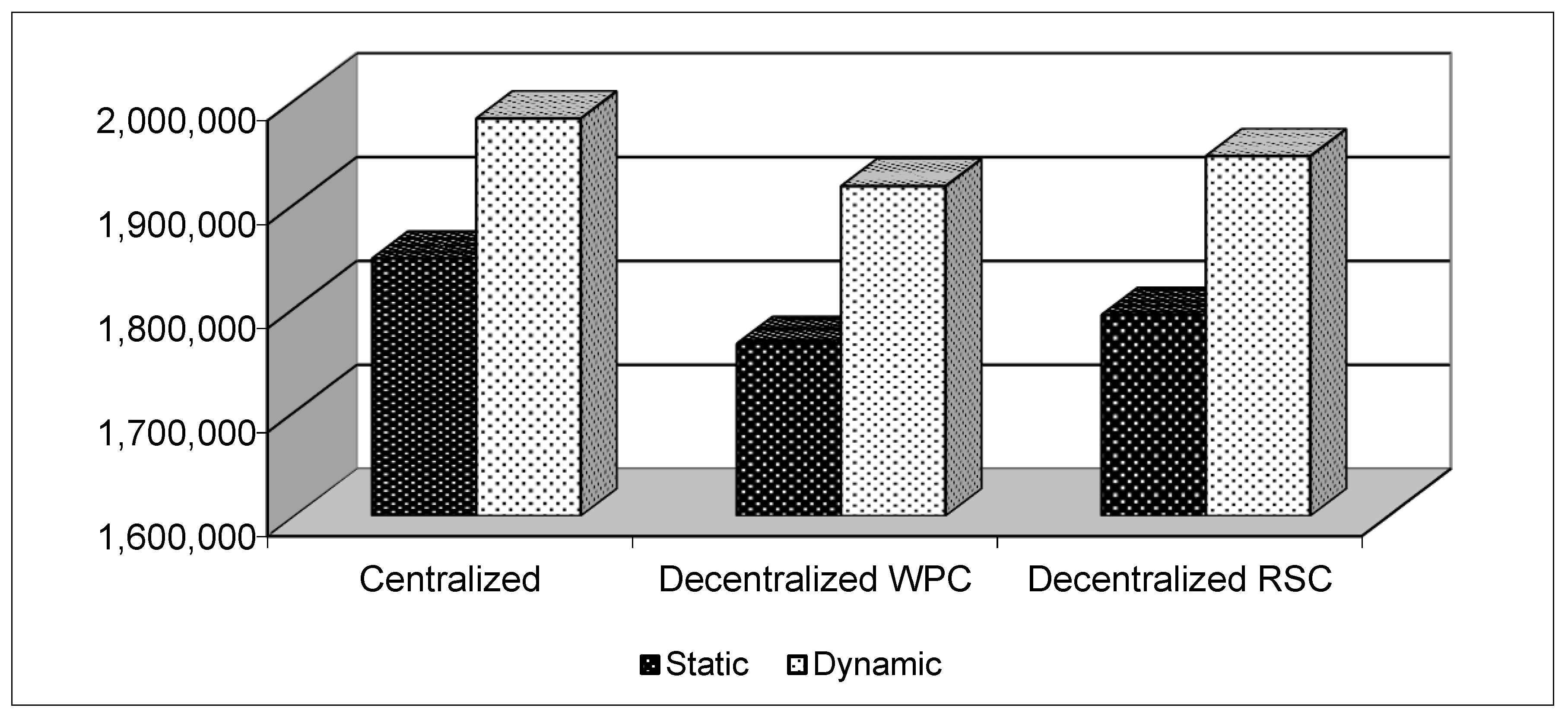
Figure 3, Figure 4 and Figure 5 below were derived by solving the static and the dynamic games optimally and analyzing the cumulative profits. Solving the dynamic games allows one to sum up the cumulative profits over time of both firms by taking into consideration the constraints linked to the state variables along the co-state variables. The outcomes of the static games were computed by solving the game in one period and multiplying the profits for the same planning horizon considered in the dynamic settings. The findings of the research are aligned with the conclusions of [32], who found the application of a theoretical game very appealing and representative of reality. They invited researchers to use theoretical tools by calibrating the parameters according to the framework.
Figure 3 reports the comparison between the cumulative profits at the end of the planning horizon. Independent of the configuration and the contract scheme, the profits obtained under the dynamic setting were always higher than those resulting under the static one. This result introduces one important novelty in the literature showing which setting, static or dynamic, should be adopted when managing SCs. The dynamic setting always prevails in economic terms. It allows developing the economies of scale in production and purchasing and, therefore, achieving the optimal level of and . Along the planning horizon, the production and purchasing rate become closer to those values, reducing the total production and purchasing costs at the end of the planning horizon. The two settings show equal gaps between actual and optimal production and purchasing level only in the beginning of the planning horizon. After that period, while the static setting still keeps the same gap until the end of the planning horizon, the dynamic one develops the economies of scale such that those costs decrease over time and confirm the statements introduced previously. Moreover, the dynamics related to the inventory policy optimize the cumulative profit over time. In the static setting, the inventories remain equal over the entire planning horizon resulting much higher that the dynamic one, i.e., not optimal at all. Finally, the dynamic setting shows an increasing price over time according to its dynamic motion. Under static settings, the price is always constant and, above all, is higher than the dynamic one. This result is always true independent of the coordination scheme and the configuration. Consequently, the demand related to the static settings is always lower than that obtainable under dynamic settings; therefore, it results in lower revenues and cumulative profits.
As confirmed by the flow of contributions in the literature, the centralized SC always results in higher cumulative profits than the decentralized one. In this sense, the centralized SC is a benchmark; whatever the coordination scheme adopted, its results can be at most attained according to the smart contract terms. The simultaneous comparison of contract schemes and configurations reveals that the RSC is highly economically attractive for coordinating decentralized SCs. Compared to the WPC, it reaches a similar level of profits to the centralized SC. This is true especially under dynamic settings. According to the literature, the RSC contract generates higher profits than the WPS. The results of this study partially confirm this previous statement. In particular, it remains valid as the comparison involves the same setting. The RSC under dynamic (static) settings makes higher cumulative profits than the WPC under dynamic (static) settings. This result is well known in the literature. One of the main novelties proposed by this research concerns the comparison of the two coordination schemes considering the setting as well. In particular, the WPC under dynamic settings generates higher cumulative profits than the WPC under a static framework. This result is quite new in the literature. Previous contributions compared the two coordination schemes by always evaluating the same setting. The choice of the setting matters consistently. In the case of a decentralized SC, the adoption of the most appropriate coordination scheme should include the selection of the right setting as well. By coordinating the SC through a WPC and working under a dynamic setting, the economic results improve significantly. The RSC fails in coordinating the SC under static settings when compared with the WPC under dynamic settings. This result finds confirmation from some theoretical results introduced by [19]. The RSC, in fact, is an effective coordination contract scheme; however, it is very expensive and difficult to administer. From this point of view, the WPC is always preferred because it is less problematic. Although RSC could appear extremely attractive, the higher part of the SC adopts WPC, losing some economic benefits expressed in terms of profit but saving time and cost for implementation and control. The results of this research show that, beyond losses and difficulties, the right choice of the coordination scheme also involves the choice of the setting; the RSC is more convenient than the WPC, while that statement contrasts with the results of this research when considering the setting.
Moreover, another important novelty concerns the comparison between decentralized SC under dynamic settings and centralized SC under a static framework. While the flow of contributions highlighted the supremacy of centralized SCs with respect to decentralized SCs, different results emerged when comparing the two settings. In particular, when coordinating SC by means of RSC under dynamic settings, the economic outcomes generated are higher than that of the centralized SC under a static framework. Additionally, the WPC under dynamic settings makes higher cumulative profits than the centralized SC under a static environment. Independent of the coordination scheme adopted, the decentralized SC under dynamic settings produces higher economic results compared to the centralized one under static settings. This result suggests a significant novelty inside the SC literature and introduces a controversial result with respect to the existing contributions. While, up to now, the literature proposed the centralized SC as a primary benchmark for comparing any other scenario, when evaluating configurations belonging to different settings, the results disconfirm part of the existing literature. In particular, this research addresses the appropriateness of investigating the SC management as a dynamic rather than a static phenomenon. In this sense, great merit goes to the use of artificial intelligence and blockchain systems. In fact, the artificial intelligence searches for optimal values of the sharing parameter that allow the firms’ decentralized strategies to mimic the outcomes of a centralized solution. Surprisingly, this job allows firms to better understand the power of a dynamic supply chain in a digital economy. The economic performance of a decentralized supply chain is considerably higher than a static centralized approach, which disregards the use of an artificial intelligence system or blockchain, as well as any form of Industry 4.0 tool. Countless variables involved in SC coordination behave differently at different instants of time; therefore, the application of the static approach generates myopic results. The dynamic investigation allows appreciating the movements and the trajectories of some variables over time such that the players act by evaluating the performance and consequently managing SCs following those changes. The particular case proposed by this research shows that the benefits generated by dynamically evaluating production and purchasing costs, inventories, and demand create controversial results with respect to 20 years of study of SC management. The decentralized SC under dynamic settings is always preferred to the centralized SC under a static environment.
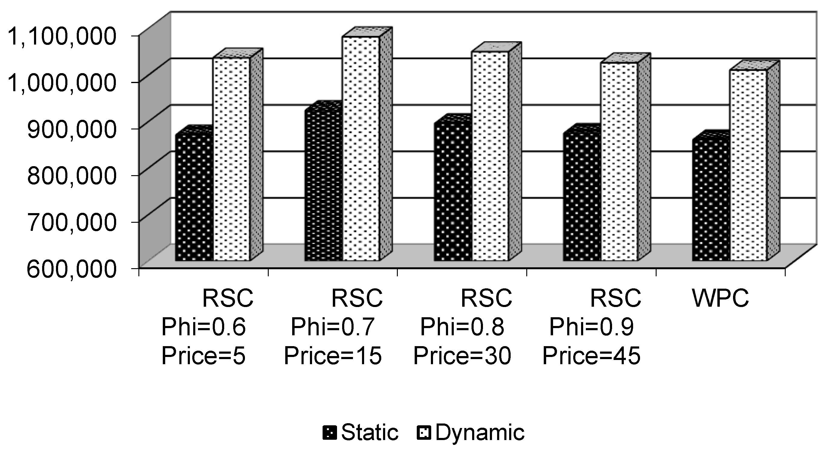
Beyond comparing the economical results from centralized and decentralized settings, this research compares the firm’s cumulative profits under decentralized settings for several values of and w. While the base case reports precise values for both parameters, here, sensitivity analysis was applied in order to investigate whether the previous statements find confirmation in the relationships between firms under decentralized settings and to identify who benefits more when implementing a particular configuration. In particular, was assumed to take values comprised in the interval (0.6, 1], while w took values comprised in the range (5, 60]. Interestingly, the artificial intelligence system proposes the use of a sharing parameter equal to 0.6, as well the minimum wholesale price. This combination can result very challenging for some companies, especially when working in a global supply chain. In fact, firms cannot control the amount of revenue that firms transfer in their transactions. Therefore, the use of blockchains helps substantially in better controlling the transaction, trusting the relationships, and making it visible to all suppliers. Finally, coordination is possible when artificial intelligence is used, as it uses the coordinated solution as a benchmark to derive the optimal contractual parameters. In this sense, we highlight that the use of blockchains and artificial intelligence for accounting duties only is a useless investment. These digital technologies should instead be used for strategic parameters like the sharing parameter and the wholesale price, requiring a high level of negotiation among suppliers.
When evaluating the effect of different combinations of and w on the manufacturer’s cumulative profits, the finding reveals particular appreciation for the RSC in eliminating the double marginalization effect. As the manufacturer sells the products at the minimum selling price that is equal to the marginal cost (w = cm = 5) and obtains a high portion of the retailer’s revenue, the supply chain takes a configuration of RSC able to mitigate the double marginalization effect and substantially increase the manufacturer’s profits. Figure 4 reports the sensitivity analysis of the two parameters for appreciating how the cumulative profit varies and identifying the most convenient configuration. Comparing these parameters from the extreme RSC with w = 5 and = 0.6 to the WPC with w = 60 and = 1, this research shows that the RSC is preferred to the WPC in most cases. The elimination of the double marginalization effect generates better results for the manufacturer with respect to the WPC that gives lower cumulative profits. This statement is highly influenced by the couple of values (w, ). For some combinations of values, the RSC always generates higher results than the WPC independent of static or dynamic settings. However, some other combinations of values disconfirm this statement. They reveal in fact that the WPC is preferred to the RSC and that the setting matters. Moreover, some combinations of parameters imply always preferring the WPC. The manufacturer should appropriately evaluate the two parameters as the economic effects change considerably.
Independent of the combination of (w, ), the retailer’s results appear quite stable. Although the RSC mitigates the double marginalization effect, that contract generates a lower benefit for the retailer. In particular, starting from the extreme configuration w = 5 and = 0.6 and considering several possible combinations, the cumulative profit does not increase as significantly as the manufacturer’s profit. When evaluating the profits within the same setting, the results of this research confirm the existing theory in the theme of SC coordination and contract; the RSC generates higher economical results that the WPC as it is able to mitigate the double marginalization effect. Nevertheless, this well-assessed statement is valid whenever the evaluation of two contract configurations involves the same setting [33]. From Figure 5, it appears quite clear that all configurations of RSC under dynamic (static) settings generate higher results than the WPC under dynamic (static) settings. Notwithstanding, the results vary consistently when comparing heterogeneous settings. In particular, according to the results obtained previously when comparing centralized and decentralized solutions, the WPC under dynamic settings generates better results than the WPC under a static environment. Consequently, the results of this research confirm the previous findings in the literature showing the supremacy of the RSC with respect to the WPC. Since the main purpose of this research concerns the comparison of static and dynamic approaches for coordinating the SC, the results disconfirm part of the existing literature. In particular, it addresses the importance of the setting when choosing the more appropriate contract scheme. In particular, for the retailer, the coordination through the RSC under static settings appears less convenient than the WPC under a dynamic environment. The RSC is difficult to administer and implement, and it does not bring more advantages than the WPC when evaluating them by considering the settings as well. The use of blockchains and artificial intelligence will surely make firms more comfortable in using complex contracts like RSC in the future.
6. Conclusions
Inspired by the contributions by the recent digital transformation, this research developed a SC game including marketing and dynamic inventory decisions. The main novelties of the paper concern the implementation of the SC game under dynamic and static settings, as well as the comparison of two contract schemes, wholesale price contract and revenue sharing contract, used for SC coordination. An artificial intelligence system supports the decision-making process and determines the optimal contract terms. In particular, the artificial intelligence uses the centralized solutions to identify the best contract clauses to be used by the firms. The blockchain allows the complexity of smart contracts to be managed such that firms can easily use digitalization in their transactions.
Our results are aligned with the literature comparing centralized and decentralized SCs within the same setting; the centralized SC under dynamic (static) settings generates higher profits than the decentralized SC under dynamic (static) settings. This result was obtained from the qualitative analysis and within the numerical resolution, and it was valid independent of the coordination scheme adopted (RSC or WPC). Nevertheless, the evaluation of the setting matters substantially. We are able to provide the following findings:
- While the existing contributions successfully assessed that the RSC is preferred to the WPC for coordinating SCs, this statement fails when comparing the WPC under dynamic settings with the RSC under static settings. In particular, the cumulative profits obtained by using WPC under dynamic settings result higher than those generated by implementing RSC under a static environment. Accordingly, SCs should be coordinated by simultaneously evaluating the contract schemes and the setting and converging toward an optimal decision. An artificial intelligence system, along with blockchain and big data, should be implemented according to these targets rather than as mere smart tools to write lines of orders.
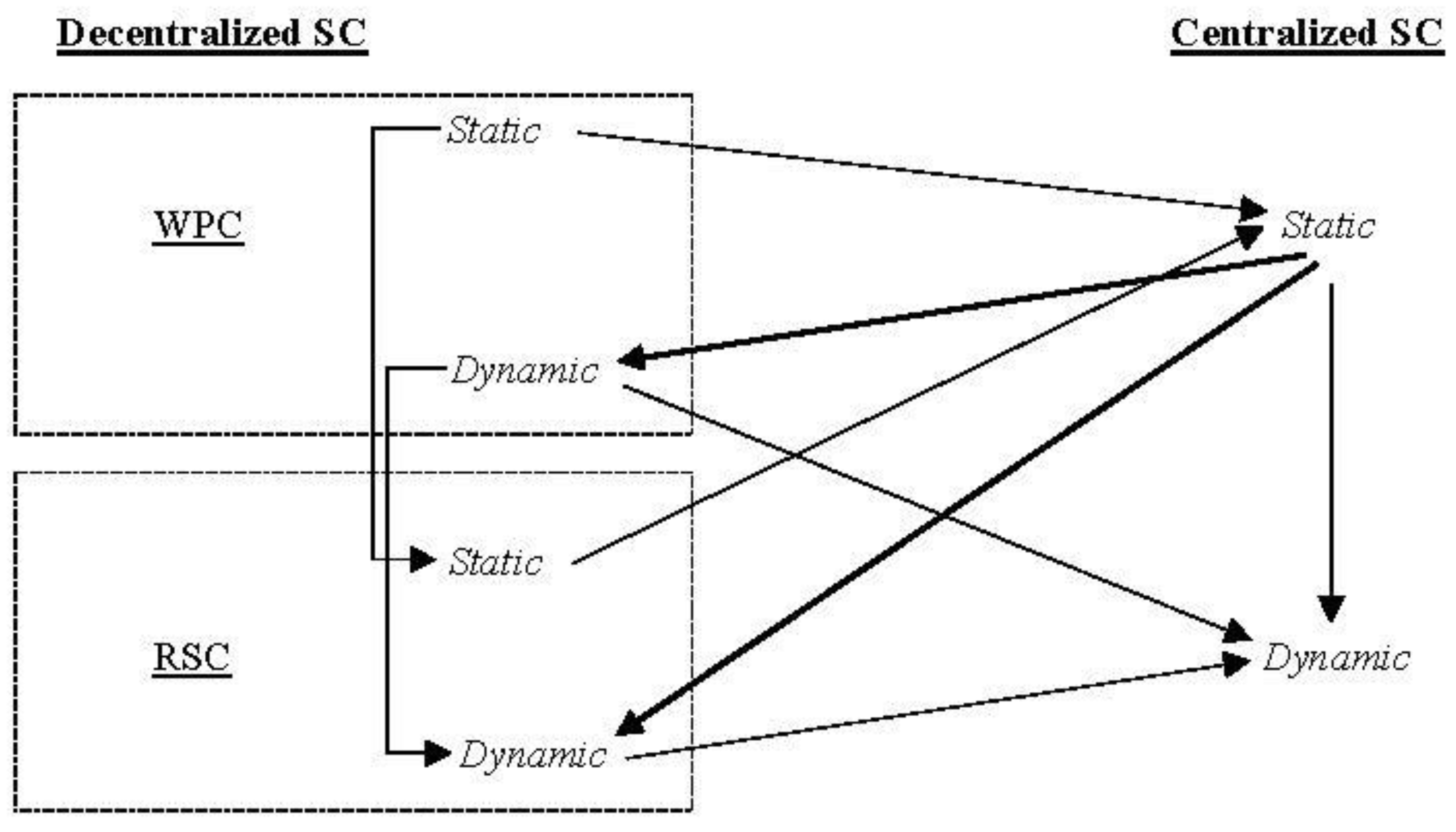
- Existing contributions clearly highlight the preference for the centralized SC to the decentralized one. We compare the cumulative profits finding that the decentralized SC under dynamic settings obtains higher profits than those obtained by the centralized SC under a static framework. This statement is true independent of the contract scheme adopted for SC coordination. This result suggests that the decision-maker cannot disregard the setting when choosing the SC configuration. Static and dynamic settings suggest an important innovation in the literature when evaluating centralized and decentralized SC compositions. Figure 6 reports the summary of our findings showing the convenience when going from one configuration to another. The bold arrows reflect the innovation due to this research, while the others concern the results already known and well established in the literature and confirmed here.
- The choice of the sharing parameter and the transferring price w determines the convenience for each player in adopting one configuration rather than another. This is particularly true for the manufacturer. When is low enough and the transferring price is equal to the marginal production cost, the RSC totally mitigates the double marginalization effect, and it is found to always be highly preferred with respect to the WPC. When the values (, w) change, the results are not obvious. The smart contracts that firms use should aim at searching for the optimal combinations of these two parameters to make SCs better off with digitalization. Our findings suggest that, beyond the choice of setting, the adequate combination of the parameters (, w) plays an important role in choosing the optimal configuration for maximizing the manufacturer’s cumulative profit.
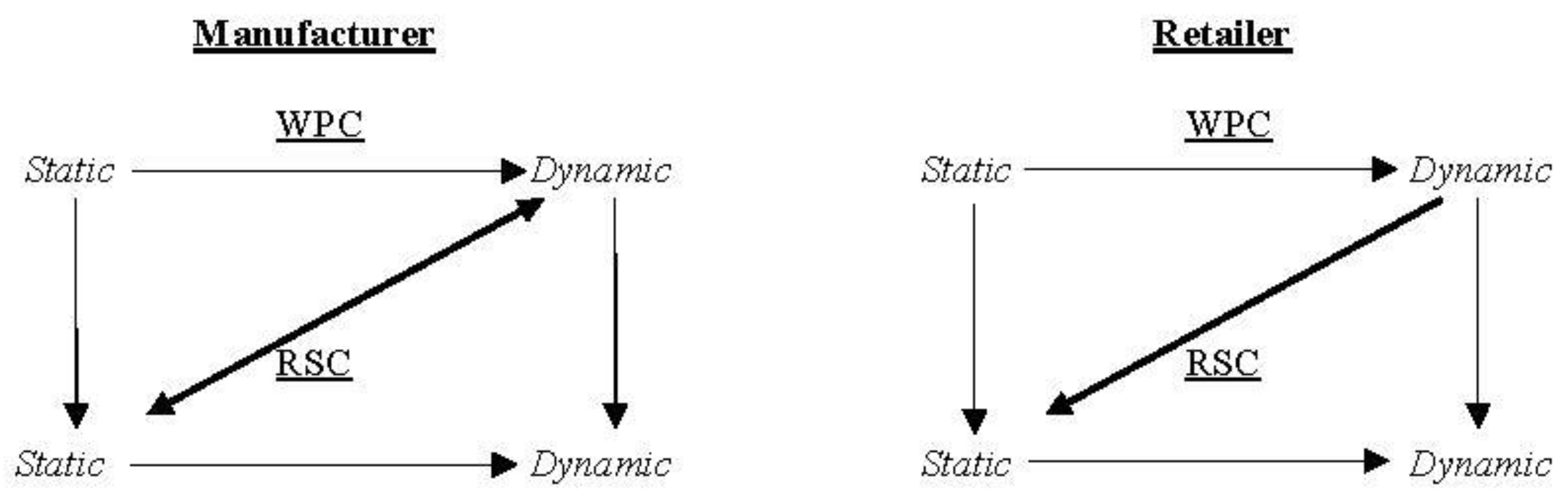
- Finally, the choice of the parameters (, w) substantially influences the retailer’s cumulative profits. Nevertheless, the retailer shows more stable and interesting results with respect to the comparison between static and dynamic settings. The implementation of the RSC is always preferred to the WPC for the higher cumulative profits generated by each combination of (, w). Notwithstanding, this result is true as long as the comparison between the two contract schemes uses the same settings. When evaluating the results of the WPC under dynamic settings with the RSC under static settings, the previous statement fails for each combination of (, w) used in the sensitivity analysis. The retailer incurs higher economic benefits by adopting WPC in dynamic settings than RSC in static settings. This result introduces a novelty in the literature. When coordinating the SC, the choice of the setting matters considerably, and the adoption of the contract scheme depends on the selection of the setting. Figure 7 reports the summary of the firms’ convenience in shifting from one configuration to another. While the results concerning the retailer are quite stable and clear, the choice of the parameters (, w) impacts the manufacturer’s decisions, which is the leading firm in terms of implementing an artificial intelligence system. Non-bold arrows illustrate the well-assessed findings in the literature, while the findings of this paper are shown in bold. Bold and double arrows represent the relationships that need further future investigations, as the results obtained are not at all definitive.
This paper is not free of limitations, which are listed to inspire future research in this area. This research most likely focuses on operational conditions. Future work can analyze the benefits of artificial intelligence and blockchains, along with smart contracts, in other contexts, such as multi-channel, omni-channel, and closed-loop SCs [34]. Future research can look to obtain real data to validate the model rather than using simulated data. Other technologies can also be evaluated in SC frameworks, such as big data, three-dimensional (3D) printing, and cloud computing.
Funding
This research received no external funding.
Conflicts of Interest
The authors declare no conflict of interest.
References
- Mentzer, J.T.; DeWitt, W.; Keebler, J.S.; Min, S.; Nix, N.W.; Smith, C.D.; Zacharia, Z.G. Defining supply chain management. J. Bus. Logist. 2001, 1, 1–25. [Google Scholar] [CrossRef]
- Kogan, K.; Tapiero, C. Supply Chain Games: Operations Management and Risk Evaluation; Springer Series in Operation Research; Springer: Berlin/Heidelberg, Germany, 2007. [Google Scholar]
- De Giovanni, P.; Ramani, V. Product cannibalization and the effect of a service strategy. J. Oper. Res. Soc. 2018, 69, 340–357. [Google Scholar] [CrossRef]
- Ramani, V.; De Giovanni, P. A two-period model of product cannibalization in an atypical Closed-loop Supply Chain with endogenous returns: The case of DellReconnect. Eur. J. Oper. Res. 2017, 262, 1009–1027. [Google Scholar] [CrossRef]
- Jeuland, A.P.; Shugan, S.M. Managing Channel Pro.ts. Mark. Sci. 1983, 2, 239–272. [Google Scholar] [CrossRef]
- Jørgensen, S. Optimal production, purchasing and pricing: A differential game approach. Eur. J. Oper. Res. 1986, 24, 64–76. [Google Scholar] [CrossRef]
- Sethi, S.P. Dynamic Optimal Control models in advertising: A survey. SIAM Rev. 1977, 19, 685–725. [Google Scholar] [CrossRef]
- Feichtinger, G.; Hartel, R.F.; Sethi, S.P. Dynamic optimal control models in advertising: Recent developments. Manag. Sci. 1994, 40, 29–31. [Google Scholar] [CrossRef]
- Dockner, E.; Jørgensen, S.; Long, N.V.; Sorger, G. Differential Games in Economics and Management Science; Cambridge University Press: Cambridge, UK, 2000. [Google Scholar]
- Erickson, G.M. Differential game models of advertising competition. Eur. J. Oper. Res. 1995, 83, 431–438. [Google Scholar] [CrossRef]
- Erickson, G.M. Empirical analysis of closed-loop duopoly advertising strategies. Manag. Sci. 1992, 38, 1732–1749. [Google Scholar] [CrossRef]
- He, X.; Prasad, A.; Sethi, S.; Gutierrez, G. A Survey of Stackelberg Differential Game Models in Supply and Marketing Channels. J. Syst. Sci. Syst. Eng. 2007, 16, 385–413. [Google Scholar] [CrossRef]
- Jørgensen, S.; Zaccour, G. Differential Games in Marketing, International Series in Quantitative Marketing; Kluwer Academic Publishers: Boston, UK, 2004. [Google Scholar]
- Taboubi, S.; Zaccour, G. Coordination Mechanisms in Marketing Channels: A Survey of Game Theory Models; Cahier du GERAD, G-2005-36; GERAD: Montreal, QC, Canada, 2005. [Google Scholar]
- De Giovanni, P. Digital Supply Chain, Design Quality and Circular Economy, in Dynamic Supply Chain Quality Models in Digital Transformation; Springer: Berlin/Heidelberg, Germany, 2020. [Google Scholar]
- De Giovanni, P. A joint maximization incentive in closed-loop supply chains with competing retailers: The case of spent-battery recycling. Eur. J. Oper. Res. 2018, 268, 128–147. [Google Scholar] [CrossRef]
- De Giovanni, P. Coordination in a distribution channel with decisions on the nature of incentives and share-dependency on pricing. J. Oper. Res. Soc. 2016, 67, 1034–1049. [Google Scholar] [CrossRef]
- De Giovanni, P.; Zaccour, G. Optimal quality improvements and pricing strategies with active and passive product returns. Omega 2019, 88, 248–262. [Google Scholar] [CrossRef]
- Cachon, G.; Netessine, S. Game theory in Supply Chain Analysis. In Handbook of Quantitative Supply Chain Analysis: Modeling in the eBusiness Era; David Simchi-Levi, S., Wu, D., Shen, Z., Eds.; Kluwer: Alphen aan den Rijn, The Netherlands, 2004. [Google Scholar]
- Taylor, T.A. Supply chain coordination under channel rebates with sales effort effects. Manag. Sci. 2002, 48, 992–1007. [Google Scholar] [CrossRef] [Green Version]
- Cachon, G.P.; Lariviere, M.A. Supply Chain coordination with revenues sharing contracts: Strength and limitations. Manag. Sci. 2005, 51, 30–44. [Google Scholar] [CrossRef] [Green Version]
- Tsay, A.A. The quantity flexibility contract and supplier-customer incentives. Manag. Sci. 1999, 45, 1339–1358. [Google Scholar] [CrossRef]
- De Giovanni, P. An optimal control model with defective products and goodwill damages. Ann. Oper. Res. 2019, 1–12. Available online: https://link.springer.com/article/10.1007/s10479-019-03176-4 (accessed on 1 October 2019).
- De Giovanni, P. Eco-Digital Supply Chain through Blockchains. In Proceedings of the 9th International Conference on Advanced in Social Science, Economics and Management Study, Rome, Italy, 7–8 December 2019. [Google Scholar]
- Zaccour, G. On the Coordination of Dynamic Marketing Channels and Two-Part Tariffs. Automatica 2008, 44, 1233–1239. [Google Scholar] [CrossRef]
- De Giovanni, P.; Karray, S.; Martín-Herrán, G. Vendor Management Inventory with consignment contracts and the benefits of cooperative advertising. Eur. J. Oper. Res. 2019, 272, 465–480. [Google Scholar] [CrossRef] [Green Version]
- Liu, B.; De Giovanni, P. Green Process Innovation Through Industry 4.0 Technologies and Supply Chain Coordination. Ann. Oper. Res. 2020, 1, 1–32. [Google Scholar]
- Wang, G.; Gunasekaran, A.; Ngai, E.W.; Papadopoulos, T. Big data analytics in logistics and supply chain management: Certain investigations for research and applications. Int. J. Prod. Econ. 2016, 176, 98–110. [Google Scholar] [CrossRef]
- Jørgensen, S. A survey of some differential games in advertising. J. Econ. Dyn. Control 1982, 4, 341–369. [Google Scholar] [CrossRef]
- Genc, T.S.; De Giovanni, P. Optimal return and rebate mechanism in a closed-loop supply chain game. Eur. J. Oper. Res. 2018, 269, 661–681. [Google Scholar] [CrossRef] [Green Version]
- Spengler, J. Vertical integration and antitrust policy. J. Political Econ. 1950, 58, 347–352. [Google Scholar] [CrossRef]
- Chalikias, M.; Skordoulis, M. Implementation of FW Lanchester’s combat model in a supply chain in duopoly: The case of Coca-Cola and Pepsi in Greece. Oper. Res. 2017, 17, 737–745. [Google Scholar]
- Preeker, T.; De Giovanni, P. Coordinating innovation projects with high tech suppliers through contracts. Res. Policy 2018, 47, 1161–1172. [Google Scholar] [CrossRef]
- De Giovanni, P.; Zaccour, G. A selective survey of game-theoretic models of closed-loop supply chains. 4OR 2019, 17, 1–44. [Google Scholar] [CrossRef]
Figure 1.
Representation of the supply chain structure.

Figure 2.
Possible combinations considering configurations, settings, and contract schemes.

Figure 3.
Comparison of cumulative profits between settings, contract schemes, and configurations.

Figure 4.
Sensitivity analysis of manufacturer’s profits.

Figure 5.
Sensitivity analysis of retailer’s profits.

Figure 6.
Summary of the comparison of centralized and decentralized supply chains (SCs).

Figure 7.
Summary of the comparison of manufacturers and retailers.


Table 1.
Technical differences between static and dynamic games.
| Static | Dynamic | |
|---|---|---|
| Planning horizon | One-shot game (t = 1) | The games have starting (t0) and ending (t) periods, or are even infinite |
| Types of games | Cooperative and non-cooperative | Cooperative and non-cooperative over open- and closed-loop frameworks |
| Mathematical computations required | System of first-order conditions | System of ordinary (partial) differential equations in open (closed)-loop games |
| Equilibrium | Best response function | Optimal control variable |
| General objective | Player payoff maximization according to the best response function | Player payoff maximization according to the optimal control variable and the optimal trajectory of the state variables |
Table 2.
Base parameters.
| a | b | hm | hr | cm | cr | pWPC | pRSC | T | |||
|---|---|---|---|---|---|---|---|---|---|---|---|
| 1000 | 20 | 0.6 | 5 | 5 | 100 | 100 | 5 | 5 | 70 | 5 | 100 |
© 2019 by the author. Licensee MDPI, Basel, Switzerland. This article is an open access article distributed under the terms and conditions of the Creative Commons Attribution (CC BY) license (http://creativecommons.org/licenses/by/4.0/).
Share and Cite
MDPI and ACS Style
De Giovanni, P. Digital Supply Chain through Dynamic Inventory and Smart Contracts. Mathematics 2019, 7, 1235. https://doi.org/10.3390/math7121235
AMA Style
De Giovanni P. Digital Supply Chain through Dynamic Inventory and Smart Contracts. Mathematics. 2019; 7(12):1235. https://doi.org/10.3390/math7121235
Chicago/Turabian StyleDe Giovanni, Pietro. 2019. "Digital Supply Chain through Dynamic Inventory and Smart Contracts" Mathematics 7, no. 12: 1235. https://doi.org/10.3390/math7121235
Note that from the first issue of 2016, this journal uses article numbers instead of page numbers. See further details here.