A Method of Solving Compressible Navier Stokes Equations in Cylindrical Coordinates Using Geometric Algebra

Abstract

A method of solution to solve the compressible unsteady 3D Navier-Stokes Equations in cylindrical co-ordinates coupled to the continuity equation in cylindrical coordinates is presented in terms of an additive solution of the three principle directions in the radial, azimuthal and z directions of flow. A dimensionless parameter is introduced whereby in the large limit case a method of solution is sought for in the tube. A reduction to a single partial differential equation is possible and integral calculus methods are applied for the case of a body force in the direction of gravity to obtain an integral form of the Hunter-Saxton equation.

1. Introduction

Compressible flow has many applications some of which are of physics, mathematics and engineering interest. In general we have two types of flows, internal and external. Internal flows in ducts are important in industry and nozzles and diffusers used in engines are also an applied area for these types of flows. In general, density changes are related to temperature changes. External flows can be important for airplanes and projectiles where compressiblilty effects are important. The Navier Stokes equations have been dealt with extensively in the literature for both analytical [1] and numerical solutions [2,3]. Some work converting the compressible Navier-Stokes equations to the Schrödinger equation in quantum mechanics by means of transformations has been carried out by Vadasz [4]. General mathematical and computational methods for compressible flow have been outlined in [5]. Methods in more general fluid mechanics are also addressed in [6]. In the context of functional analysis it has been shown in [7] that generally the motion of a compressible fluid with fixed initial velocity field and constant initial density converges to that of an incompressible fluid as its sound speed goes to infinity. Some analytical methods such as in [8] have been successfully carried out for one and two dimensional isentropic unsteady compressible flow. In the present work I introduce a new procedure to write the compressible unsteady Navier Stokes equations with a general spatial and temporal varying density term in terms of an additive solution of the three principle directions in the radial, azimuthal and z directions of flow. This procedure can be used in physics and engineering to simplify a complex system of PDE to a simpler one such as complex multiphase flows [9] and other areas in physics using Geometric Algebra, such as for example the study of the Maxwell equations. In mathematics, the method leads to the present work which shows the necessary conditions for the full solution of the system of equations for compressible flow to blowup at a certain time for certain types of initial conditions and also implications of using assumptions for necessary and physically meaningful functional forms of density. Following the general procedure, a dimensionless parameter is introduced whereby in the large limit case a method of solution is sought for in the tube. It is concluded that the total divergence of the flow can be expressed as the integral with respect to time of the line integral of the dot product of inertial and azimuthal velocity. The line integral can be evaluated on a contour that is annular and traces the boundary layer as time increases in the flow. A reduction to a single partial differential equation is possible and integral calculus methods are applied for the case of a body force directed downwards with gravity to obtain an integral form of the Hunter-Saxton equation. A specific density function that is exponential in time and having characteristics of a pulse that propagates radially and axially in the tube and can be interpreted as having a large density gradient in time and in space is used.

2. A New Composite Velocity Formulation

The 3D compressible cylindrical unsteady Navier-Stokes equations are written in expanded form, for each component, $u_r$, $u_{\theta }$ and $u_z$:

$$\begin{array}{c}\frac{\partial u_r}{\partial t}+u_r\frac{\partial u_r}{\partial r}+\frac{u_{\theta }}{r}\frac{\partial u_r}{\partial \theta }-\frac{u_{\theta }^2}{r}+u_z\frac{\partial u_r}{\partial z}-\frac{\mu }{\rho }\left(-\frac{u_r}{r^2}+\frac{{\partial }^2{u}_r}{\partial r^2}+\frac{1}{r}\frac{\partial u_r}{\partial r}+\frac{1}{r^2}\frac{{\partial }^2{u}_r}{\partial {\theta }^2}-\frac{2}{r^2}\frac{\partial u_{\theta }}{\partial \theta }+\frac{{\partial }^2{u}_r}{\partial z^2}\right)-\\ \frac{\mu }{3\rho }\frac{\partial }{\partial r}\left(\frac{\partial u_r}{\partial r}+\frac{1}{r}\frac{\partial u_r}{\partial \theta }+\frac{\partial u_r}{\partial z}\right)+\frac{1}{\rho }\frac{\partial p}{\partial r}-F{g}_r=0\end{array}$$

(1)

$$\begin{array}{c}\frac{\partial u_{\theta }}{\partial t}+u_r\frac{\partial u_{\theta }}{\partial r}+\frac{u_{\theta }}{r}\frac{\partial u_{\theta }}{\partial \theta }+\frac{1}{r}{u}_r{u}_{\theta }+u_z\frac{\partial u_{\theta }}{\partial z}-\frac{\mu }{\rho }\left(-\frac{u_{\theta }}{r^2}+\frac{{\partial }^2{u}_{\theta }}{\partial r^2}+\frac{1}{r}\frac{\partial u_{\theta }}{\partial r}+\frac{1}{r^2}\frac{{\partial }^2{u}_{\theta }}{\partial {\theta }^2}+\frac{2}{r^2}\frac{\partial u_r}{\partial \theta }+\frac{{\partial }^2{u}_{\theta }}{\partial z^2}\right)-\\ \frac{1}{r}\frac{\mu }{3\rho }\frac{\partial }{\partial \theta }\left(\frac{\partial u_{\theta }}{\partial r}+\frac{1}{r}\frac{\partial u_{\theta }}{\partial \theta }+\frac{\partial u_{\theta }}{\partial z}\right)+\frac{1}{\rho r}\frac{\partial p}{\partial \theta }-F{g}_{\theta }=0\end{array}$$

(2)

$$\begin{array}{c}\frac{\partial u_z}{\partial t}+u_r\frac{\partial u_z}{\partial r}+\frac{u_{\theta }}{r}\frac{\partial u_z}{\partial \theta }+u_z\frac{\partial u_z}{\partial z}-\frac{\mu }{\rho }\left(\frac{{\partial }^2{u}_z}{\partial r^2}+\frac{1}{r}\frac{\partial u_z}{\partial r}+\frac{1}{r^2}\frac{{\partial }^2{u}_z}{\partial {\theta }^2}+\frac{{\partial }^2{u}_z}{\partial z^2}\right)-\\ \frac{\mu }{3\rho }\frac{\partial }{\partial z}\left(\frac{\partial u_z}{\partial r}+\frac{1}{r}\frac{\partial u_z}{\partial \theta }+\frac{\partial u_z}{\partial z}\right)+\frac{1}{\rho }\frac{\partial p}{\partial z}-F{g}_z=0\end{array}$$

(3)

where $u_r$ is the radial component of velocity, $u_{\theta }$ is the azimuthal component and $u_z$ is the velocity component in the direction along tube, $\rho$ is density, $\mu$ is dynamic viscosity, $F{g}_r$, $F{g}_{\theta }$, $F{g}_z$ are body forces on fluid. The total gravity force vector is expressed as $\overrightarrow{F_T}=(F{g}_r,F{g}_{\theta },F{g}_z)$.

The following relationships between starred and non-starred dimensional quantities together with a non-dimensional quantity $\delta$ are used:

$$u_r=\frac{1}{{\delta }^2}{u}_r^{*}$$

(4)

$$u_{\theta }=\frac{1}{\delta }{u}_{\theta }^{*}$$

(5)

$$u_z=\frac{1}{\delta }{u}_z^{*}$$

(6)

$$r=\frac{r^{*}}{\delta }$$

(7)

$$\theta ={\theta }^{*}$$

(8)

$$z=\frac{1}{\delta }{z}^{*},t=\delta t^{*}$$

(9)

c a constant is defined below, $\delta =-\frac{1}{r^{*}}\frac{\partial \rho }{\partial {\theta }^{*}}{\left(\frac{\partial \rho }{\partial r^{*}}+\frac{\rho }{r^{*}}\right)}^{-1}$ as part of the continuity equation (Equation (12)). The solution of this equation in terms of $\rho$ is of the form $\frac{f_{\rho }\left(\frac{\theta \delta +ln\left(r\right)}{\delta },z,t\right)}{r}$, for general function $f_{\rho }$, I first set $f_{\rho }=B\left(r\right)\left(1+\frac{{\mathrm{e}}^{-\frac{{(\theta \delta +ln(-r))}^2}{\delta }}}{r}\right){\mathrm{e}}^{ct-\mathit{mz}}$, which is a Dirac type pulse as $\delta$ gets arbitrarily large. For the second type of density function of small amplitude, $f_{\rho }=B\left(r\right)\theta \left(1-\frac{{\mathrm{e}}^{-{\left(1-ln\left(r\right)\right)}^2}}{r}\right){\mathrm{e}}^{ct-\mathit{mz}}$, where $B\left(r\right)$ is a function of compact support on an interval $[0,r_w]$. For the second choice of $f_{\rho }$ the density $\rho$ is defined everywhere in tube when $\theta =ϵ$ is small for $\delta$ large and in addition $f_{\rho }$ solves the pde in $\delta$ and $\rho$ above for both types.This will eliminate two of the nonlinear terms in the Navier Stokes equations below for $\delta$ sufficiently large and negative.

Using Equations (4)–(9),multiplying Equations (1)–(3) by cartesian unit vectors $\overrightarrow{e_{r^{*}}}=(1,0,0)$, $\overrightarrow{e_{{\theta }^{*}}}=(0,1,0)$ and $\overrightarrow{k}=(0,0,1)$ respectively and adding Equations (1)–(3) gives the following equation, for the resulting composite vector $\overrightarrow{L_1}=\frac{1}{{\delta }^2}{u}_{r^{*}}^{*}\overrightarrow{e_{r^{*}}}+\frac{1}{\delta }{u}_{{\theta }^{*}}^{*}\overrightarrow{e_{{\theta }^{*}}}+\frac{1}{\delta }{u}_{z^{*}}^{*}\overrightarrow{k}$,

$$\begin{array}{c}\delta \left(\frac{\partial \overrightarrow{L_1}}{\partial t}+\frac{u_{r^{*}}^{*}}{{\delta }^2}\frac{\partial \overrightarrow{L_1}}{\partial r^{*}}+\frac{u_{{\theta }^{*}}^{*}}{\delta r^{*}}\frac{\partial \overrightarrow{L_1}}{\partial {\theta }^{*}}+\frac{1}{\delta }{u}_{z^{*}}^{*}\frac{\partial \overrightarrow{L_1}}{\partial z^{*}}-\frac{1}{{\delta }^2{r}^{*}}{u}_{{\theta }^{*}}^{{*}^2}\overrightarrow{e_{r^{*}}}+\frac{1}{{\delta }^3{r}^{*}}{u}_{r^{*}}^{*}{u}_{{\theta }^{*}}^{*}\overrightarrow{e_{{\theta }^{*}}}\right)-\\ \frac{\mu }{\rho }\left(-{\delta }^2\frac{\overrightarrow{L_1}}{{r^{*}}^2}+{\delta }^2\frac{{\partial }^2\overrightarrow{L_1}}{\partial {r^{*}}^2}+{\delta }^2\frac{1}{r^{*}}\frac{\partial \overrightarrow{L_1}}{\partial r^{*}}+{\delta }^2\frac{1}{{r^{*}}^2}\frac{{\partial }^2\overrightarrow{L_1}}{\partial {{\theta }^{*}}^2}+\frac{2{\delta }^2}{{r^{*}}^2}\left(\frac{1}{{\delta }^2}\frac{\partial u_{r^{*}}^{*}}{\partial {\theta }^{*}}\overrightarrow{e_{{\theta }^{*}}}-\frac{1}{\delta }\frac{\partial u_{{\theta }^{*}}^{*}}{\partial {\theta }^{*}}\overrightarrow{e_{r^{*}}}\right)+{\delta }^2\frac{{\partial }^2\overrightarrow{L_1}}{\partial {z^{*}}^2}\right)-\\ \frac{\mu }{3\rho }\frac{\partial }{\partial r^{*}}\left(\frac{\partial u_{r^{*}}^{*}}{\partial r^{*}}+\frac{1}{r^{*}}\frac{\partial u_{r^{*}}^{*}}{\partial {\theta }^{*}}+\frac{\partial u_{r^{*}}^{*}}{\partial z^{*}}\right)\overrightarrow{e_{r^{*}}}-\frac{\delta }{r^{*}}\frac{\mu }{3\rho }\frac{\partial }{\partial {\theta }^{*}}\left(\frac{\partial u_{{\theta }^{*}}^{*}}{\partial r^{*}}+\frac{1}{r^{*}}\frac{\partial u_{{\theta }^{*}}^{*}}{\partial {\theta }^{*}}+\frac{\partial u_{{\theta }^{*}}^{*}}{\partial z^{*}}\right)\overrightarrow{e_{{\theta }^{*}}}\\ -\delta \frac{\mu }{3\rho }\frac{\partial }{\partial z^{*}}\left(\frac{\partial u_{z^{*}}^{*}}{\partial r^{*}}+\frac{1}{r^{*}}\frac{\partial u_{z^{*}}^{*}}{\partial {\theta }^{*}}+\frac{\partial u_{z^{*}}^{*}}{\partial z^{*}}\right)\overrightarrow{k}+\delta \frac{1}{\rho }\frac{\partial p}{\partial r^{*}}\overrightarrow{e_{r^{*}}}+\delta \frac{1}{r^{*}\rho }\frac{\partial p}{\partial {\theta }^{*}}\overrightarrow{e_{{\theta }^{*}}}+\delta \frac{1}{\rho }\frac{\partial p}{\partial z^{*}}\overrightarrow{k}-\overrightarrow{F_T}=0\end{array}$$

(10)

Furthermore one can take the cross product of Equation (10) with $\overrightarrow{e_{r^{*}}}$ and $\overrightarrow{e_{{\theta }^{*}}}$ to form two equations respectively where in the second case multiplication by $\delta$ to cancel squared nonlinear terms, $-\frac{1}{{\delta }^2{r}^{*}}{u}_{{\theta }^{*}}^{{*}^2}\overrightarrow{e_{r^{*}}},\frac{1}{{\delta }^3{r}^{*}}{u}_{r^{*}}^{*}{u}_{{\theta }^{*}}^{*}\overrightarrow{e_{{\theta }^{*}}}$, leads to,

$$\begin{array}{c}\delta \left(\frac{\partial \overrightarrow{L_A}}{\partial t}+\frac{u_{r^{*}}^{*}}{{\delta }^2}\frac{\partial \overrightarrow{L_A}}{\partial r^{*}}+\frac{u_{{\theta }^{*}}^{*}}{\delta r^{*}}\frac{\partial \overrightarrow{L_A}}{\partial {\theta }^{*}}+\frac{1}{\delta }{u}_{z^{*}}^{*}\frac{\partial \overrightarrow{L_A}}{\partial z^{*}}\right)+{\delta }^{-2}\frac{u_{{\theta }^{*}}^{*}}{r^{*}}\frac{-\rho \overline{L}-\frac{\partial \rho }{\partial t}-u_{z^{*}}^{*}\frac{\partial \rho }{\partial z^{*}}}{\frac{\partial \rho }{\partial r^{*}}}\overrightarrow{k}-\\ \frac{\mu }{\rho }\left(-{\delta }^2\frac{\overrightarrow{L_A}}{{r^{*}}^2}+{\delta }^2\frac{{\partial }^2\overrightarrow{L_A}}{\partial {r^{*}}^2}+{\delta }^2\frac{1}{r^{*}}\frac{\partial \overrightarrow{L_A}}{\partial r^{*}}+{\delta }^2\frac{1}{{r^{*}}^2}\frac{{\partial }^2\overrightarrow{L_A}}{\partial {{\theta }^{*}}^2}+\frac{2{\delta }^2}{{r^{*}}^2}\left(\frac{1}{{\delta }^2}\frac{\partial u_{r^{*}}^{*}}{\partial {\theta }^{*}}\overrightarrow{k}-\frac{1}{\delta }\frac{\partial u_{{\theta }^{*}}^{*}}{\partial {\theta }^{*}}\overrightarrow{k}\right)+{\delta }^2\frac{{\partial }^2\overrightarrow{L_A}}{\partial {z^{*}}^2}\right)+\\ +\frac{\delta }{r^{*}}\frac{\mu }{3\rho }\frac{\partial }{\partial {\theta }^{*}}\left(\frac{\partial u_{{\theta }^{*}}^{*}}{\partial r^{*}}+\frac{1}{r^{*}}\frac{\partial u_{{\theta }^{*}}^{*}}{\partial {\theta }^{*}}+\frac{\partial u_{{\theta }^{*}}^{*}}{\partial z^{*}}\right)\overrightarrow{k}+\delta \frac{\mu }{3\rho }\frac{\partial }{\partial z^{*}}\left(\frac{\partial u_{z^{*}}^{*}}{\partial r^{*}}+\frac{1}{r^{*}}\frac{\partial u_{z^{*}}^{*}}{\partial {\theta }^{*}}+\frac{\partial u_{z^{*}}^{*}}{\partial z^{*}}\right)\overrightarrow{e_{{\theta }^{*}}}-\\ \delta \frac{\mu }{3\rho }\frac{\partial }{\partial r^{*}}\left(\frac{\partial u_{r^{*}}^{*}}{\partial r^{*}}+\frac{1}{r^{*}}\frac{\partial u_{r^{*}}^{*}}{\partial {\theta }^{*}}+\frac{\partial u_{r^{*}}^{*}}{\partial z^{*}}\right)\overrightarrow{k}+{\delta }^2\frac{\mu }{3\rho }\frac{\partial }{\partial z^{*}}\left(\frac{\partial u_{z^{*}}^{*}}{\partial r^{*}}+\frac{1}{r^{*}}\frac{\partial u_{z^{*}}^{*}}{\partial {\theta }^{*}}+\frac{\partial u_{z^{*}}^{*}}{\partial z^{*}}\right)\overrightarrow{e_{r^{*}}}-\delta \frac{1}{r^{*}\rho }\frac{\partial p}{\partial {\theta }^{*}}\overrightarrow{k}-\\ \delta \frac{1}{\rho }\frac{\partial p}{\partial z^{*}}\overrightarrow{e_{{\theta }^{*}}}+{\delta }^2\frac{1}{\rho }\frac{\partial p}{\partial r^{*}}\overrightarrow{k}-{\delta }^2\frac{1}{\rho }\frac{\partial p}{\partial z^{*}}\overrightarrow{e_{r^{*}}}+\overrightarrow{F_T}=0\end{array}$$

(11)

where $\overrightarrow{L_A}=-u_{z^{*}}^{*}\overrightarrow{e_{r^{*}}}-\frac{1}{\delta }{u}_{z^{*}}^{*}\overrightarrow{e_{\theta }^{*}}+\frac{1}{\delta }(u_{r^{*}}^{*}-u_{{\theta }^{*}}^{*})\overrightarrow{k}$, $\overrightarrow{L_A}=\overrightarrow{L_1}\times \overrightarrow{e_{r^{*}}}+\delta \overrightarrow{L_1}\times \overrightarrow{e_{\theta }^{*}}$ and continuity equation, Equation (12) below has been used. Equation (10) is sufficient to carry out the subsequent analysis.

3. A Solution Procedure for $\mathit{\delta }$ Arbitrarily Large in Quantity

Multiplication of Equation (10) by $\frac{\rho }{\delta }$ and Equation (12) below by $\frac{\overrightarrow{L_1}}{\delta }$, addition of the resulting equations [9], and using the ordinary product rule of differential multivariable calculus a form as in Equation (13) is obtained whereby I set $\overrightarrow{a}=\rho \overrightarrow{L_1}$.

The continuity equation in cylindrical co-ordinates is

$$\frac{\partial \rho }{\partial t}+\frac{1}{\delta }{u}_{r^{*}}^{*}\frac{\partial \rho }{\partial r^{*}}+\frac{u_{{\theta }^{*}}^{*}}{r^{*}}\frac{\partial \rho }{\partial {\theta }^{*}}+u_{z^{*}}^{*}\frac{\partial \rho }{\partial z^{*}}=-\rho \left(\frac{1}{\delta }\frac{u_{r^{*}}^{*}}{r^{*}}+\frac{1}{\delta }\frac{\partial u_{r^{*}}^{*}}{\partial r^{*}}+\frac{1}{r^{*}}\frac{\partial u_{{\theta }^{*}}^{*}}{\partial {\theta }^{*}}+\frac{\partial u_{z^{*}}^{*}}{\partial z^{*}}\right)=-\rho \overline{L}$$

(12)

$$\rho \frac{\partial \overrightarrow{a}}{\partial t}+\overrightarrow{a}·\nabla \overrightarrow{a}+{\rho }^2\overrightarrow{b}\nabla ·\overrightarrow{b}=\mu \left(\delta \right)\left({\nabla }^2\overrightarrow{b}+\frac{1}{3}\nabla (\nabla ·\overrightarrow{b})\right)+\nabla P+\overrightarrow{F_T}$$

(13)

where $\mu \left(\delta \right)=\mu \delta$.

Taking the geometric product in the previous equation with the inertial vector term,

$$\overrightarrow{f}=\overrightarrow{a}·\nabla \overrightarrow{a}$$

(14)

where $\overrightarrow{b}=\frac{\overrightarrow{a}}{\rho }$ is defined, where in the context of Geometric Algebra, the following scalar and vector grade equations arise,

$$\overrightarrow{f}·\left({\rho }^2\frac{\partial \overrightarrow{b}}{\partial t}+\rho \overrightarrow{b}\frac{\partial \rho }{\partial t}\right)+{\Vert \overrightarrow{f}\Vert }^2+\overrightarrow{b}·\overrightarrow{f}{\rho }^2\nabla ·\overrightarrow{b}=\mu \left(\delta \right)\overrightarrow{f}·{\nabla }^2\overrightarrow{b}+\frac{\mu \left(\delta \right)}{3}\overrightarrow{f}·\nabla (\nabla ·\overrightarrow{b})+\overrightarrow{f}·\nabla P$$

(15)

$${\rho }^2\frac{\partial \overrightarrow{b}}{\partial t}+\rho \overrightarrow{b}\frac{\partial \rho }{\partial t}+\overrightarrow{b}{\rho }^2\nabla ·\overrightarrow{b}=\mu \left(\delta \right)\left({\nabla }^2\overrightarrow{b}+\frac{1}{3}\nabla (\nabla ·\overrightarrow{b})\right)+\nabla P+\overrightarrow{F_T}$$

(16)

The geometric product of two vectors [10], is defined by $\overrightarrow{A}\overrightarrow{B}=\overrightarrow{A}·\overrightarrow{B}+\overrightarrow{A}\times \overrightarrow{B}$.

Taking the divergence of Equation (16) results in

$$\begin{array}{c}{\rho }^2\frac{\partial }{\partial t}\left(\nabla ·\overrightarrow{b}\right)+\rho \frac{\partial \rho }{\partial t}\nabla ·\overrightarrow{b}+\overrightarrow{b}·\nabla (\rho \frac{\partial \rho }{\partial t})+\nabla ·(\overrightarrow{b}{\rho }^2\nabla ·\overrightarrow{b})=\nabla ·\left(\mu \left(\delta \right){\nabla }^2(\overrightarrow{b}\right)+\\ \frac{\mu \left(\delta \right)}{3}\nabla ·\left(\nabla (\nabla ·\overrightarrow{b})\right)+\nabla ·\left(\nabla P\right)+\nabla ·\overrightarrow{F_T}\end{array}$$

(17)

Upon multiplication of Equation (17) by,

$$H=\frac{\rho \overrightarrow{b}·\overrightarrow{f}}{\frac{\partial \rho }{\partial t}}$$

(18)

the resulting equation is

$$\begin{array}{c}{\rho }^{2}H\frac{\partial }{\partial t}(\nabla ·\overrightarrow{b})+{\rho }^2\overrightarrow{b}·\overrightarrow{f}\nabla ·\overrightarrow{b}+H\overrightarrow{b}·\nabla (\rho \frac{\partial \rho }{\partial t})+H\nabla ·(\overrightarrow{b}{\rho }^2\nabla ·\overrightarrow{b})=\\ \mu \left(\delta \right)H\nabla ·{\nabla }^2\overrightarrow{b}+\frac{\mu \left(\delta \right)}{3}H\nabla ·(\nabla (\nabla ·\overrightarrow{b}))+H\nabla ·(\nabla P)+H\nabla ·\overrightarrow{F_T}\end{array}$$

(19)

which results upon using Equation (15) in,

$$\begin{array}{c}{\rho }^{2}H\frac{\partial }{\partial t}(\nabla ·\overrightarrow{b})-\overrightarrow{f}·\left({\rho }^2\frac{\partial \overrightarrow{b}}{\partial t}+\rho \overrightarrow{b}\frac{\partial \rho }{\partial t}\right)-{\Vert \overrightarrow{f}\Vert }^2-\mu \left|\delta \right|\overrightarrow{f}·{\nabla }^2\overrightarrow{b}-\frac{\mu \left|\delta \right|}{3}\overrightarrow{f}·\nabla (\nabla ·\overrightarrow{b})-\overrightarrow{f}·\nabla P+H\overrightarrow{b}·\nabla (\rho \frac{\partial \rho }{\partial t})+\\ H\nabla ·(\overrightarrow{b}{\rho }^2\nabla ·\overrightarrow{b})=-\mu \left|\delta \right|H(\nabla ·{\nabla }^2\overrightarrow{b})-\frac{\mu \left|\delta \right|}{3}H\nabla ·(\nabla (\nabla ·\overrightarrow{b}))+H\nabla ·\left(\nabla P\right)+H\nabla ·\overrightarrow{F_T}\end{array}$$

(20)

The continuity equation is written in terms of $\overrightarrow{b}$ as,

$$\frac{1}{\delta }\frac{\partial \rho }{\partial t}+\rho \nabla ·\overrightarrow{b}+\overrightarrow{b}·\nabla \rho =0$$

(21)

and

$$\nabla ·\overrightarrow{b}=-\frac{1}{\delta \rho }\frac{\partial \rho }{\partial t}-\nabla \rho ·\overrightarrow{b}$$

(22)

where the following compact expression is given,

$$Y^{*}=\nabla ·\overrightarrow{b}$$

(23)

Multiplying by ${(\overrightarrow{f}·\overrightarrow{f})}^{-1}$ in Equation (20) and, using properties of third derivatives involving the gradient and in particular the fact that the Laplacian of the divergence of a vector field is equivalent to the divergence of the Laplacian of a vector field, leads to the following form,

$$\begin{array}{c}{W}^{*}\frac{\partial Y^{*}}{\partial t}-G(\rho ,\frac{\partial \rho }{\partial t})W^{*}-F(\rho ,\frac{\partial \rho }{\partial t})\overrightarrow{b}\overrightarrow{f}(1+\overrightarrow{f}·\nabla P)-{\rho }^{-2}V\left(\mu \right)\left|\delta \right|W^{*}{\nabla }^2\left(Y^{*}\right)-\overrightarrow{b}\overrightarrow{f}\frac{\partial \rho }{\partial t}\frac{{\rho }^{-1}}{{\Vert \overrightarrow{f}\Vert }^2}\overrightarrow{f}·\left(\frac{\partial \overrightarrow{b}}{\partial t}\right)+\mathsf{\Omega }+\\ \overrightarrow{b}\overrightarrow{f}\frac{\partial \rho }{\partial t}\frac{{\rho }^{-3}}{{\Vert \overrightarrow{f}\Vert }^2}\mu \left|\delta \right|\overrightarrow{f}·{\nabla }^2\overrightarrow{b}+\overrightarrow{b}\overrightarrow{f}\frac{\partial \rho }{\partial t}\frac{{\rho }^{-3}}{{\Vert \overrightarrow{f}\Vert }^2}\frac{\mu \left|\delta \right|}{3}\overrightarrow{f}·\nabla (\nabla ·\overrightarrow{b})-{\rho }^{-2}\overrightarrow{b}\overrightarrow{f}\frac{1}{{\Vert \overrightarrow{f}\Vert }^2}\overrightarrow{b}·\overrightarrow{f}\nabla ·\left(\overrightarrow{b}{\rho }^2\nabla ·\overrightarrow{b}+\nabla P+\overrightarrow{F_T}\right)=0\end{array}$$

(24)

where $\mathsf{\Omega }={\rho }^{-2}H\overrightarrow{b}·\nabla \left(\rho \frac{\partial \rho }{\partial t}\right)$ in Equation (24) and,

$$W^{*}=\left(\frac{\overrightarrow{f}·\overrightarrow{b}}{{\Vert \overrightarrow{f}\Vert }^2}\overrightarrow{f}\right)\overrightarrow{b}=\left(\frac{\overrightarrow{f}·\overrightarrow{b}}{{\Vert \overrightarrow{f}\Vert }^2}\overrightarrow{f}\right)·\overrightarrow{b}+\left(\frac{\overrightarrow{f}·\overrightarrow{b}}{{\Vert \overrightarrow{f}\Vert }^2}\overrightarrow{f}\right)\times \overrightarrow{b}=\xi +\overrightarrow{f}\times \left(\frac{\overrightarrow{f}·\overrightarrow{b}}{{\Vert \overrightarrow{f}\Vert }^2}\overrightarrow{b}\right)$$

(25)

This involves the vector projection of $\overrightarrow{b}$ onto $\overrightarrow{f}$ which is written in the conventional form,

$${proj}_{\mathbf{f}}\mathbf{b}=\frac{\mathbf{f}·\mathbf{b}}{{\Vert \mathbf{f}\Vert }^2}\mathbf{f}$$

(26)

Equation (24) can be written compactly as

$$\frac{\partial Y^{*}}{\partial t}-G(\rho ,\frac{\partial \rho }{\partial t})-{\rho }^{-2}V\left(\mu \right)\left|\delta \right|{\nabla }^2{Y}^{*}-{\rho }^{-2}{\nabla }^{2}P={\rho }^{-2}\frac{U_{\overrightarrow{f}}\left[\mathbf{Q}(\rho ,\frac{\partial \rho }{\partial t},\overrightarrow{b},\frac{\partial \overrightarrow{b}}{\partial t},\nabla P,\overrightarrow{F_T})+\overrightarrow{f}\right]}{U_{\overrightarrow{f}}\overrightarrow{b}}$$

(27)

where $U_{\overrightarrow{f}}\overrightarrow{\xi }$ is the scalar projection for $\overrightarrow{b}$, $G=\frac{1}{{\rho }^2}{\left(\frac{\partial \rho }{\partial t}\right)}^2$, $\mathbf{Q}$ (a differential operator defined by Equations (16) and (24)) and hence for a constant $\alpha$,

$$\frac{\partial Y^{*}}{\partial t}-G(\rho ,\frac{\partial \rho }{\partial t})-{\rho }^{-2}V\left(\mu \right)\left|\delta \right|{\nabla }^2{Y}^{*}-{\rho }^{-2}{\nabla }^{2}P={\rho }^{-2}\frac{\Vert \mathbf{Q}(\rho ,\frac{\partial \rho }{\partial t},\overrightarrow{b},\frac{\partial \overrightarrow{b}}{\partial t},\nabla P,\overrightarrow{F_T})+\overrightarrow{f}\Vert }{\Vert \overrightarrow{b}\Vert }=\alpha {\rho }^{-2}\ge 0$$

(28)

with solution in terms of a function $\mathcal{B}$,

$$Y^{*}=\nabla ·\overrightarrow{b}=\mathcal{B}(\alpha ,r,\theta ,z,t)$$

(29)

If the rate of change of $\rho$ with respect to t is changing exponentially in time as $f_{\rho }=N\left(r\right){\mathrm{e}}^{ct-\mathit{mz}}$ $(\rho =f_{\rho }$ and $c=\frac{1}{\delta }<0,m<0)$, where $N\left(r\right)$ is either of two density type functions defined in the beginning of this paper, it may be proven that $\mathcal{B}$ is written in terms of a separable function, if ${\rho }^{-2}{\nabla }^{2}P$ is chosen to be negligible. and I obtain,

$$Y\left(r,\theta ,z,t\right)={\mathit{F}}_1\left(r\right){\mathit{F}}_2\left(\theta \right){\mathit{F}}_3\left(z\right){\mathit{F}}_4\left(t\right)-1/4\frac{\alpha \left(\delta \right)}{V\left(\mu \left(\delta \right)\right){\delta }^3{\mathit{C}}_2}\left(\frac{{\mathit{C}}_1}{r}+{\mathit{C}}_2{r}^2+{\mathit{C}}_{3}r\right)$$

(30)

where ${\mathit{F}}_{\mathit{i}}$ are the separable parts of the function, $C_1$, $C_2$, $C_3$, are arbitrary constants, and as $C_2\to \infty$,

$$M\left(r\right)=1/4\frac{\alpha \left(\delta \right)}{V\left(\mu \left(\delta \right)\right){\delta }^3{\mathit{C}}_2}\left(\frac{{\mathit{C}}_1}{r}+{\mathit{C}}_2{r}^2+{\mathit{C}}_{3}r\right)=1/4\frac{\alpha \left(\delta \right)r^2}{{\delta }^{3}V\left(\mu \left(\delta \right)\right)}$$

(31)

For $c^2$ approaching zero and using the properties of the norm,

$$\Vert \left[{\mathit{Y}}^{*}\left(r,\theta ,z,t\right)-{\mathit{F}}_1\left(r\right){\mathit{F}}_2\left(\theta \right){\mathit{F}}_3\left(z\right){\mathit{F}}_4\left(t\right)\right]\overrightarrow{b}-\left[\mathbf{Q}\left(\rho ,\frac{\partial \rho }{\partial t},\overrightarrow{b},\frac{\partial \overrightarrow{b}}{\partial t},\nabla P,\overrightarrow{F_T}\right)+\overrightarrow{f}\right]\Vert =0$$

(32)

Furthermore using the property for a norm on a vector space of continuous functions (since away from $r=0$), $\Vert A\Vert =0$ iff $A=0$, and Equation (16) and the second line of Equation (24) gives,

$$\begin{array}{c}\left[{\mathit{Y}}^{*}\left(r,\theta ,z,t\right)-{\mathit{F}}_1\left(r\right){\mathit{F}}_2\left(\theta \right){\mathit{F}}_3\left(z\right){\mathit{F}}_4\left(t\right)\right]\overrightarrow{b}+\\ \left[-2\frac{\partial \overrightarrow{b}}{\partial t}-\frac{1}{\rho }\overrightarrow{b}\frac{\partial \rho }{\partial t}-F(\rho ,\frac{\partial \rho }{\partial t})(\overrightarrow{f}+\overrightarrow{F_T})\right]-{\rho }^{-2}\overrightarrow{b}\nabla ·\left(-\overrightarrow{b}{\rho }^2\nabla ·\overrightarrow{b}+\overrightarrow{F_T}\right)=0\end{array}$$

(33)

where $\Vert \left[{\mathit{Y}}^{*}\left(r,\theta ,z,t\right)-{\mathit{F}}_1\left(r\right){\mathit{F}}_2\left(\theta \right){\mathit{F}}_3\left(z\right){\mathit{F}}_4\left(t\right)\right]\Vert \to 0$, for $\delta \to -\infty$, with $\mu$ chosen such that $V\left(\mu \right(\delta \left)\right)=\alpha \left(\delta \right)$ (here it can be proved that the viscosity is a function of density which is a Dirac pulse function, also in general it can be proven that Equation (28) with viscosity as a function of small amplitude type density function can have a similar form as in Equation (30)) for a new form of $M\left(r\right)$. Next continuing with Equation (33),

$$\begin{array}{c}\left[-2\frac{\partial \overrightarrow{b}}{\partial t}-\frac{1}{\rho }\overrightarrow{b}\frac{\partial \rho }{\partial t}-(c\overrightarrow{f_b}+\overrightarrow{F_T})\right]-{\rho }^{-2}\overrightarrow{b}\nabla ·\overrightarrow{F_T}=0\end{array}$$

(34)

where $F(\rho ,\frac{\partial \rho }{\partial t})={\rho }^{-3}\frac{\partial \rho }{\partial t}$. $\mathsf{\Omega }$ in Equation (24) vanishes due to assumption on rate of change of density with respect to t and $c^2\approx 0$, and finally Equation (22) has been used with a calculation done to show that the expression reduces in going from Equation (33) to Equation (34).

Also, $F(\rho ,\frac{\partial \rho }{\partial t})\overrightarrow{f}={\rho }^{-3}\frac{\partial \rho }{\partial t}{\rho }^2\overrightarrow{b}·\nabla \overrightarrow{b}={\rho }^{-1}\frac{\partial \rho }{\partial t}\overrightarrow{b}·\nabla \overrightarrow{b}=c\overrightarrow{f_b}.$

For large r it can be proven that $F1\left(r\right)$ is decaying as a $J_0$ Bessel function and $F\ne 0$ is an increasing function radially in tube ($r>0$) with the following resulting upon taking the curl of Equation (34),

$$-2\frac{\partial }{\partial t}\nabla \times \overrightarrow{b}-c\nabla \times \overrightarrow{f_b}-\nabla \times \left({\rho }^{-2}\overrightarrow{b}\nabla ·\overrightarrow{F_T}\right)=0$$

(35)

where the conservative gravity force drops out.

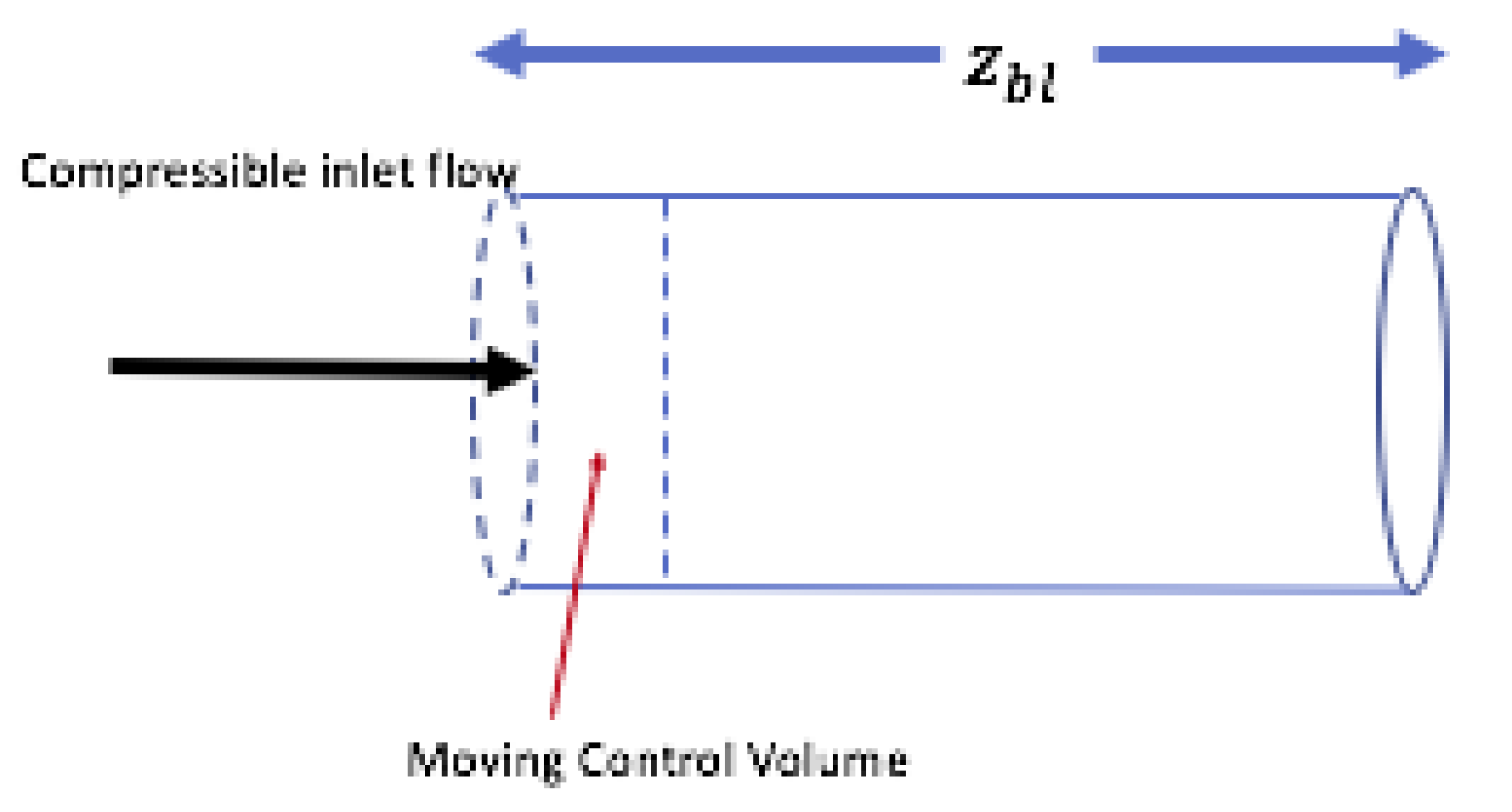
Multiply Equation (35) by the normal vector $cos\left(\theta \right)\overrightarrow{a}$ which is the normal component of $\overrightarrow{a}$ at wall of moving control volume (CV) in Figure 1,

$$cos\left(\theta \right)\overrightarrow{a}·\left[-2\frac{\partial }{\partial t}\nabla \times \overrightarrow{b}-c\nabla \times \overrightarrow{f_b}-\nabla \times \left({\rho }^{-2}\overrightarrow{b}\nabla ·\overrightarrow{F_T}\right)\right]=0$$

(36)

Recalling Divergence theorem and Stoke’s theorem, for general $\mathbf{F}$,

$$\begin{array}{cc}\hfill \underset{V}{\int \int \int }(\nabla ·\mathbf{F})dV& =\underset{S\left(V\right)}{{\displaystyle ∯}}\mathbf{F}·\widehat{\mathbf{n}}dS\hfill \end{array}$$

$$\underset{S}{\int \int }(\nabla \times \mathbf{F})·d\mathbf{S}={\oint }_C\mathbf{F}\left(\mathbf{r}\right)·d\mathbf{r}$$

(37)

where C is the contour of a circle in control volume of tube and S consists of all surfaces of control volume.

Defining the following vector field,

$$\overrightarrow{W}=-\frac{\partial }{\partial t}\nabla \times \overrightarrow{b}-\frac{1}{2}\nabla \times \left({\rho }^{-2}\overrightarrow{b}\nabla ·\overrightarrow{F_T}\right),$$

(38)

$$\begin{array}{cc}\hfill \underset{S\left(V\right)}{{\displaystyle ∯}}\mathbf{W}·\widehat{\mathbf{n}}dS& =\underset{V}{\int \int \int }(\nabla ·\mathbf{W})dV\hfill \end{array}$$

(39)

$$\begin{array}{c}=\frac{c}{2}{\oint }_C{\mathbf{f}}_{\mathbf{b}}\left(\mathbf{r}\right)·d\mathbf{r}\hfill \end{array}$$

(40)

where $\widehat{\mathbf{n}}=cos\left(\theta \right)\overrightarrow{a}$, and Stoke’s theorem has been used. Applying Stoke’s theorem to $\overrightarrow{W}$, hence $\overrightarrow{b}$.

$$\frac{c}{2}{\oint }_C\overrightarrow{f_b}\left(\mathbf{r}\right)·\overrightarrow{T}ds=-{\oint }_C(\frac{\partial \overrightarrow{b}}{\partial t}+\frac{1}{2}{\rho }^{-2}\overrightarrow{b}\nabla ·\overrightarrow{F_T})·d\mathbf{r}$$

(41)

where $\overrightarrow{T}$ is unit tangent vector to closed curve C and $ds$ is arc length,

$${\oint }_C(\frac{c}{2}\overrightarrow{f_b}\left(\mathbf{r}\right)+\frac{\partial \overrightarrow{b}}{\partial t}+\frac{1}{2}{\rho }^{-2}\overrightarrow{b}\nabla ·\overrightarrow{F_T})·d\mathbf{r}=0$$

(42)

The third term in the parenthesis in Equation (42) is integrated by parts for line integral and I obtain the following,

$${\oint }_C(\frac{c}{2}\overrightarrow{f_b}(\mathbf{r})+\frac{\partial \overrightarrow{b}}{\partial t}-\frac{1}{2}\overrightarrow{F_T}\nabla ·({\rho }^{-2}\overrightarrow{b}))·d\mathbf{r}=0$$

(43)

Parametrizing the circle as $r=g\left(\theta \right)$ in polar coordinates it can be proven that the line integral in Equation (43) is,

$${\oint }_C(c\frac{f_{b_1}}{2}+\frac{\partial b_1}{\partial t}-\frac{1}{2}{F}_{T_1}\nabla ·({\rho }^{-2}\overrightarrow{b}))·d\theta -{\oint }_C(c\frac{f_{b_2}}{2}+\frac{\partial b_2}{\partial t}-\frac{1}{2}{F}_{T_2}\nabla ·({\rho }^{-2}\overrightarrow{b}))·dr=0$$

(44)

The normal form of Green’s theorem can be used for the line integral in Equation (44), setting first,

$$M=c\frac{f_{b_1}}{2}+\frac{\partial b_1}{\partial t}-\frac{1}{2}{F}_{T_1}\nabla ·({\rho }^{-2}\overrightarrow{b})$$

(45)

$$N=c\frac{f_{b_2}}{2}+\frac{\partial b_2}{\partial t}-\frac{1}{2}{F}_{T_2}\nabla ·({\rho }^{-2}\overrightarrow{b})$$

(46)

The line integral in Equation (44) is equal to the following,

$${\int \int }_R\left(\frac{\partial M}{\partial r}+\frac{\partial N}{\partial \theta }\right)drd\theta$$

(47)

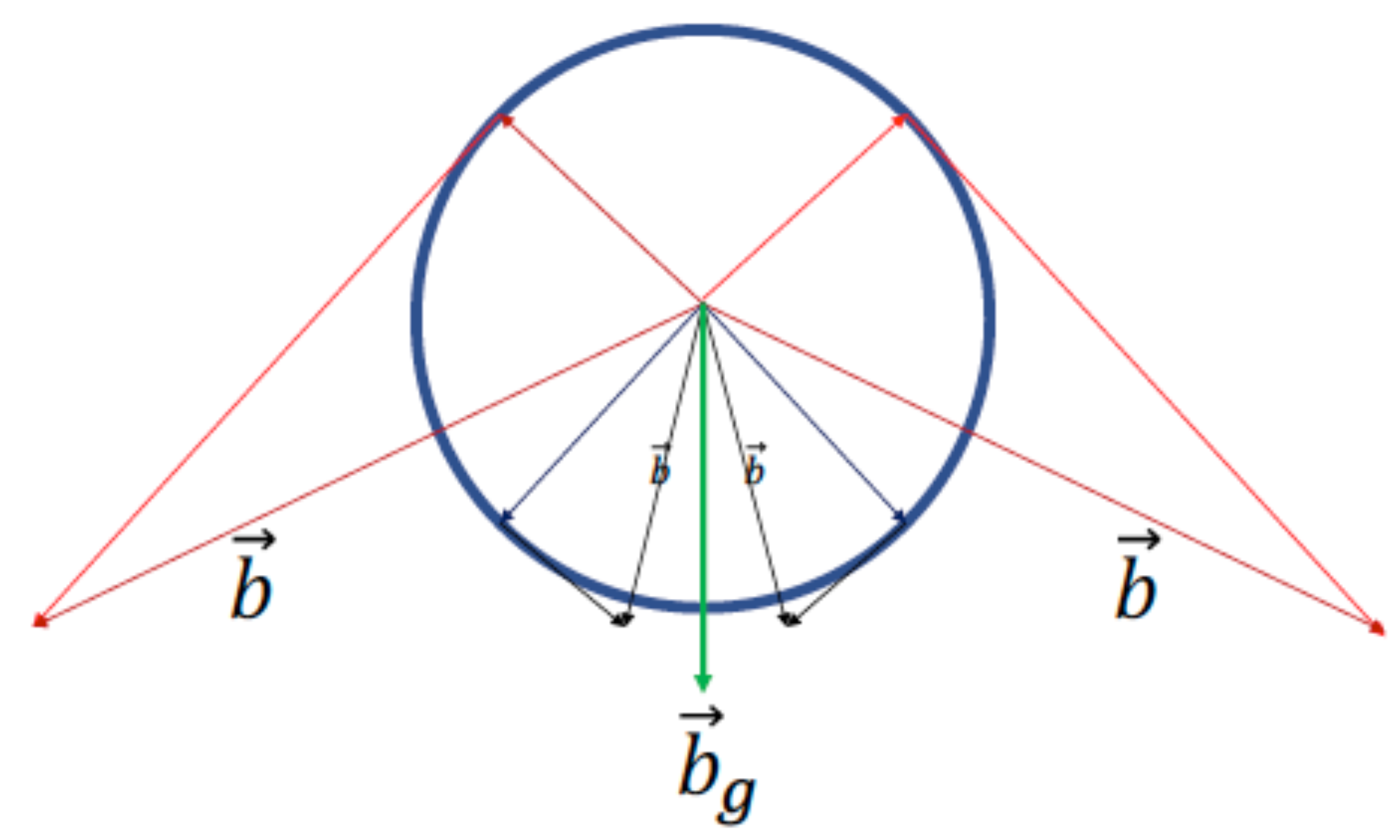
where M and N are given by Equations (45) and (46) respectively and R is the open disk with boundary C. The gravity force $F_{T_1}$ is expressed as follows,

$$F_{T_1}=-\nabla \varphi =-g\nabla h=g\nabla \Vert (\overrightarrow{b}Tcos(\frac{\pi }{4}-\theta ))\Vert$$

(48)

where $\varphi$ is a potential function, h is the negative height in the direction of the vector $\overrightarrow{b_g}$ in Figure 2, T is a time constant and g is gravity constant. Also $cos(\frac{\pi }{4}-\theta )\Vert \overrightarrow{b}\Vert =\Vert \overrightarrow{b_g}\Vert$ at the vertical vector $\overrightarrow{b_g}$ in Figure 2. It follows that Equation (47) becomes,

$${\int \int }_R\left[-\frac{1}{2}gT\frac{\partial }{\partial r}\left[\frac{1}{r^2}{\left(\frac{\partial b_g}{\partial \theta }\right)}^2{\rho }^{-2}\right]+{(\frac{c}{r}{b}_g{b}_{g_{\theta }}+\frac{\partial b_g}{\partial t})}_{\theta }\right]drd\theta$$

(49)

$${\int \int }_R\left[-\frac{1}{2}gT\frac{\partial }{\partial r}\left[{\left(\frac{\partial b_g}{\partial \theta }\right)}^2\frac{1}{r^2}{\left(1+\frac{{\mathrm{e}}^{-{\left(1-ln\left(r\right)\right)}^2}}{r}\right)}^{-2}\right]+{(\frac{c}{r}{b}_g{b}_{g_{\theta }}+\frac{\partial b_g}{\partial t})}_{\theta }\right]drd\theta$$

(50)

$${\int \int }_R\left[-\frac{1}{2}gT\left[{\left(\frac{\partial b_g}{\partial \theta }\right)}^2\frac{4{\mathrm{e}}^{-{\left(ln\left(r\right)-1\right)}^2}ln\left(r\right)-4{\mathrm{e}}^{-{\left(ln\left(r\right)-1\right)}^2}-2r}{r{\left(r+{\mathrm{e}}^{-{\left(ln\left(r\right)-1\right)}^2}\right)}^3}\right]+{(\frac{c}{r}{b}_g{b}_{g_{\theta }}+\frac{\partial b_g}{\partial t})}_{\theta }\right]drd\theta$$

(51)

$$\begin{array}{c}{\int \int }_R-\frac{1}{2}gT\left(4{\mathrm{e}}^{-{\left(ln\left(r\right)-1\right)}^2}ln\left(r\right)-4{\mathrm{e}}^{-{\left(ln\left(r\right)-1\right)}^2}-2r\right)+\\ \frac{\partial }{\partial \theta }\left[r{\left(r+{\mathrm{e}}^{-{\left(ln\left(r\right)-1\right)}^2}\right)}^3\frac{c}{r}{b}_g{b}_{g_{\theta }}+r{\left(r+{\mathrm{e}}^{-{\left(ln\left(r\right)-1\right)}^2}\right)}^3\frac{\partial b_g}{\partial t}\right]drd\theta \end{array}$$

(52)

For $\delta \to \infty$ the function $b_2=b_g(\theta ,t)$ and $b_1=b_1(r,t)\approx 0$, and thus for $c<0$ small, integration in r on the interval $[0,r_w]$, where $r_w$ is near the wall in control volume,

$${\int }_0^{2\pi }\left[-W_2\frac{1}{2}gT{c}^{-1}{\left(\frac{\partial b_g}{\partial \theta }\right)}^2+\frac{\partial }{\partial \theta }{\left[W_1{b}_g{b}_{g_{\theta }}+r{c}^{-1}{W}_3\frac{\partial b_g}{\partial t})\right]}_{\theta }\right]drd\theta$$

(53)

In the above analysis I have integrated the second term in second line of Equation (52) wiith respect to r and have obtained,

$$\begin{array}{c}{W}_1\left(r\right)=3/2A\sqrt{\pi }\mathrm{erf}\left(-5/2+ln\left(r\right)\right)+3/4B\sqrt{\pi }\sqrt{2}\mathrm{erf}\left(1/2\left(2ln\left(r\right)-3\right)\sqrt{2}\right)+\\ 1/6C\sqrt{3}\sqrt{\pi }\mathrm{erf}\left(1/6\left(6ln\left(r\right)-7\right)\sqrt{3}\right)+1/4r^4+C\end{array}$$

(54)

where A, B and C are constants. Letting $r=\frac{r_w}{\delta }$ and $\delta \to \infty$, I obtain a general non-zero constant $W_1=-3A\sqrt{(}\pi )(1/2)-3B\sqrt{(}\pi )\sqrt{(}2)(1/4)-(1/6)C\sqrt{(}3\left)\sqrt{(}\pi \right)+C$. Integrating the first term in Equation (52) with respect to r following the same procedure as in previous step, the result is that I obtain a general nonzero constant $W_2$. The same is true for the third term in Equation (52) where I have a non-zero constant $W_3$.

Choosing constants in $W_1$, $W_2$ and $W_3$ such that $W_2\frac{1}{2}gT{c}^{-1}=1/2$, $W_1=1$ and $c^{-1}{W}_3$ = 1, the resulting equation obtained is the Hunter-Saxton PDE.

4. The Hunter-Saxton Equation

Substituting $f_2$ and $F_{T_1}$ into Equations (45) and (46) since $F_{T_2}=0$ and $f_1,b_1$ terms are negligible in the boundary layer(Recall $u_r=u_r^{*}/{\delta }^2$ then one can obtain an integral form of the Hunter-Saxton equation using Equation (53),

$${\left(b_{2_t}^{*}+b_2^{*}{b}_{2_{\theta }}^{*}\right)}_{\theta }=\frac{1}{2}{b_{2_{\theta }}^{*}}^2$$

(55)

It is of interest that a more complicated partial differential equation is obtained upon taking $F_{T_2}$ to be non zero and thus defining a rotational force related to the vorticity of the fluid elements in the boundary layer. In the interval $[0,t]$ the boundary layer starts to form at $t=0$ and reaches maximum height at time t. See Figure 1 and Figure 3 for control volume over the growth of the boundary layer and contours between boundary layer and tube wall. The time dependence is shown in the inertial term $\overrightarrow{f}$. The right side of Equation (40) consists of nonlinear inertial term $\overrightarrow{f}$ and Equation (39) shows the dependence on these gradients and rate of change of curl of $\overrightarrow{b}$ with respect to t.

5. Discussion

It is known that there exist sufficient conditions for the blowup in time of smooth solutions to the compressible Navier-Stokes equations in arbitrary space dimensions with initial density of compact support [11]. The present work focuses on the compressible Navier Stokes equations in 3D in cylindrical coordinates. It has been shown that this system is reducible to the Hunter-Saxton equation which is used to model nematic liquid crystals and this nonlinear PDE also blows up in finite time if the initial boundary condition is set equal to a non-monotone increasing function [12].

6. Conclusions

An attempt has been made to reduce the compressible Navier Stokes equations coupled to the continuity equation in cylindrical co-ordinates to a simpler problem in terms of an additive solution of the three principle directions in the radial, azimuthal and z directions of flow. A dimensionless parameter is introduced whereby in the large limit case a method of solution is sought for in the tube. By seeking an additive solution using the continuity equation and the simplified vector equation obtained by a similar procedure, using the product rule of differentiable calculus, and using Geometric Algebra as a starting point, it follows through analysis that the integral of total divergence of a specific vector field over time can be expressed as the integral with respect to time of the line integral of the dot product of inertial and azimuthal velocity. The line integral can be evaluated on a contour that is annular and traces the boundary layer as time increases in the flow. It has been shown that a reduction of the 3D compressible unsteady Navier-Stokes equations to a single partial differential equation is possible and integral calculus methods are applied for the case of a body force in the direction of gravity to obtain an integral form of the Hunter-Saxton equation. The radial flow due to the gravitational pull at the centre of the disk in Figure 2 does not result in an immediate radial flow downwards towards the wall of the tube. Rather, the fluid compresses near the centre of the disk where the gravitational force exists (and is greatest there due to a nonuniform mass distribution where it is assumed that the mass is greatest at the center of disk) and hence the density increases locally in response to the force. The compressed fluid expands against the neighbouring fluid particles causing the neighboring fluid particles to compress and set in motion a wave pulse that travels downwards towards the wall in Figure 2 [13]. It is worthy to note that for this reason the density must be not-monotone increasing, i.e., it must either be a Dirac pulse or Gaussian-like wave function (i.e., of compact support), or a pulse of small amplitude.The reduction obtained in this paper allows one to analyze the Hunter-Saxton PDE which gives great insight into the nature of nematic liquid crystals which can be formed due to large temporal and spatial gradients in density. The viscosity can thus be used in describing the flow with boundary layer formation near the surface of the tube. Both a dynamic and rotational viscosity are related to dissipation of energy and on reorientation of the NLC director. The Hunter-Saxton system is known to blow up in finite time when the function used as an initial condition is a not-monotone increasing function. Since the density is necessarily to be either an infinite Dirac function or a pulse of finite and small amplitude, it is concluded that the governing system of compressible non-linear 3D Navier Stokes equations coupled to the space-time density dependent continuity equation will blow up in finite time. A restriction of $F_{T_2}=0$ was made and one can consider a more general body force than has been shown where in addition there is a rotational force applied. Future studies are required to examine this problem.

References

1. Pereira, L.M.; Guerrero, J.S.P.; Cotta, R.M. Integral transformation of the Navier Stokes equations in cylindrical geometry. Comput. Mech. 1998, 21, 60–70. [Google Scholar] [CrossRef]
2. Taylor, C.; Hughes, T.G. Finite Element Programming of the Navier Stokes Equations; Pineridge Press: Swansea, UK, 1981; Available online: https://trove.nla.gov.au/work/25314368?q&versionId=30518049 (accessed on 24 January 2018).
3. MacCormack, R.W. A Numerical Method for Solving the Equations of Compressible Viscous Flow. AIAA J. 1982, 20, 1275–1281. [Google Scholar] [CrossRef]
4. Vadasz, P. Rendering the Navier-Stokes equations for a compressible fluid into the Schrödinger Equation for quantum mechanics. Fluids 2016, 1, 18. [Google Scholar] [CrossRef]
5. Feistauer, M.; Felcman, J.; Straskraba, I. Mathematical and Computational Methods for Compressible Flow; Oxford University Press: Oxford, UK, 2004. [Google Scholar]
6. Batchelor, G.K. An Introduction to Fluid Dynamics; Cambridge University Press: Cambridge, UK, 1967. [Google Scholar]
7. Ebin, D.G. Motion of a slightly compressible fluid. Proc. Natl. Acad. Sci. USA 1975, 72, 539–542. [Google Scholar] [CrossRef] [PubMed]
8. Cai, R. Some Explicit analytical solutions of unsteady compressible flow. J. Fluids Eng. 1998, 120, 760–764. [Google Scholar] [CrossRef]
9. Moschandreou, T. A New Analytical Procedure to Solve Two Phase Flow in Tubes. Math. Comput. Appl. 2018, 23, 26. [Google Scholar] [CrossRef]
10. Doran, C.; Lasenby, A. Geometric Algebra for Physicists; Cambridge University Press: Cambridge, UK, 2003. [Google Scholar]
11. Xin, Z. Blowup of Smooth Solutions to the Compressible Navier-Stokes Equation with Compact Density. Commun. Pure Appl. Math. 1998, 51, 229–240. [Google Scholar] [CrossRef]
12. Hunter, J.K.; Saxton, R. Dynamics of Director Fields. SIAM J. Appl. Math. 1991, 51, 1498–1521. [Google Scholar] [CrossRef]
13. Morisson, F.A. Compressible Fluids; Michigan Technological University: Houghton, MI, USA, 2004; pp. 94–98. [Google Scholar]
Figure 1. Compressible Viscous Flow in a Tube, z b l is the distance to achieve maximum boundary layer height.
Mathematics 07 00126 g001
Figure 2. Vector b g which is pointing in the direction of increasing gravitational force. The right angle triangles show vector addition as expressed by solution, L 1 = b = 1 δ 2 u r * * e r * + 1 δ u θ * * e θ * .
Mathematics 07 00126 g002
Figure 3. A typical set of contour lines between edge of boundary layer and tube wall.
Mathematics 07 00126 g003
Figure 4. Vectors a , c , d as well as d 1 and d 2 which are pointing in the direction of increasing gravitational force. (Appendix A).
Mathematics 07 00126 g004