A Multi-Objective Particle Swarm Optimization Algorithm Based on Gaussian Mutation and an Improved Learning Strategy

Abstract

Obtaining high convergence and uniform distributions remains a major challenge in most metaheuristic multi-objective optimization problems. In this article, a novel multi-objective particle swarm optimization (PSO) algorithm is proposed based on Gaussian mutation and an improved learning strategy. The approach adopts a Gaussian mutation strategy to improve the uniformity of external archives and current populations. To improve the global optimal solution, different learning strategies are proposed for non-dominated and dominated solutions. An indicator is presented to measure the distribution width of the non-dominated solution set, which is produced by various algorithms. Experiments were performed using eight benchmark test functions. The results illustrate that the multi-objective improved PSO algorithm (MOIPSO) yields better convergence and distributions than the other two algorithms, and the distance width indicator is reasonable and effective.

1. Introduction

Multi-objective optimization problems (MOPs) are very common in engineering and other areas of research, such as economics, finance, production scheduling, and aerospace engineering. It is very difficult to solve these problems because they usually involve several conflicting objectives. Generally, the optimal solution of MOPs is a set of optimal solutions (known as a Pareto optimal set), which differs from the solution of single-objective optimization (with only one optimal solution) [1]. Some classical optimization methods (weighted methods, goal programming methods, etc.) require the problem functions to be differentiable and are required to run multiple times with the hope of finding different solutions. In recent years, the multi-objective optimization evolutionary algorithm (MOEA) has become a popular method for solving MOPs, and it has garnered scholarly interest around the world [2]. Many representative MOEAs, such as multiple objective genetic algorithm (MOGA) [3], non-dominated sorting genetic algorithm II (NSGA-II) [4], strength pareto evolutionary algorithm (SPEA) [5] and pareto archived evolution strategy (PAES) [6], have been presented.

Over the past decade, the particle swarm optimization algorithm (PSO) has been used to solve MOPs, and a number of multi-objective PSO algorithms have been suggested. Some studies have shown that the modified PSO algorithm can effectively solve the MOPs and that the non-dominated solution set of the algorithm is much closer to the true Pareto optimal front. Coello and Pultdo [7] incorporated a special mutation operator that enriches the exploratory capabilities. Sierra and Coello [8] proposed the OMOPSO algorithm, which places the whole population into three subpopulations with the same size and uses different mutation operators within different subpopulations. This algorithm improves the exploration ability of the particles. Reddy and Kumar [9] proposed an elitist-mutation multi-objective PSO (EM-MOPSO) algorithm with a strategic mechanism that effectively explores the feasible search space and speeds up the search for the true Pareto optimal region. Leong and Yen [10] proposed a dynamic population multiple-swarm MOPSO algorithm that uses an adaptive local archive to improve the diversity within each swarm. Yen and Leong [11] also proposed a dynamic population multiple-swarm MOPSO algorithm in which the number of swarms is adaptively adjusted throughout the search process via the proposed dynamic swarm strategy. The strategy allocates an appropriate number of swarms to support convergence and diversity criteria among the swarms as required. Chen, Zou, and Wang [12] presented a multi-objective endocrine particle swarm optimization algorithm (MOEPSO) in which the hormone (RH), released by the endocrine system, is encoded as a particle swarm and is then supervised by the corresponding stimulating hormone. Lin et al. [13] introduced a novel MOPSO algorithm using multiple search strategies (MMOPSO), and a decomposition approach was used to transform MOPs into a set of aggregation problems. Then, each particle was accordingly assigned to optimize each aggregation problem. A multi-objective vortex particle swarm optimization (MOVPSO) method was proposed in [14] based on the emerging properties of a swarm to simulate motion with diversity control via collaborative mechanisms using linear and circular movements. The parallel cell coordinate system (PCCS) in self-adaptive MOPSO [15] is used to select global and personal bests, maintain archives and adjust flight parameters. Knight et al. [16] presented a spreading mechanism to promote diversity in MOPSO. Cheng et al. [17] presented a hybrid multi-objective particle swarm optimization that combines the canonical PSO search with a teaching–learning-based optimization (TLBO) algorithm to promote diversity and improve the search ability. Overall, for any improved MOPSO algorithm, the search ability is determined by the neighbouring topological structure, and the convergence rate depends on the dominance relationship.

In this paper, we introduce a new multi-objective PSO algorithm based on Gaussian mutation and an improved learning strategy to solve MOPs. The main new contributions of this work can be summarized as: (1) Gaussian mutation throw points strategy to improve the uniformity of external archives and current populations; (2) For MOPs, it is difficult to select the $g_{\mathrm{best}}$ value of velocity and update the formula. Unlike other MOPSOs, that often randomly select a solution from the external archive as the global optimal solution $g_{\mathrm{best}}$, we present different learning strategies to update the individual positions of the non-dominated and dominated solutions; (3) To further measure the distribution width, the indicator $DW$ is proposed.

The remainder of this paper is organized as follows. In Section 2, we describe the multi-objective optimization. Thereafter, in Section 3, we present a multi-objective improved PSO algorithm (MOIPSO). Section 4 outlines the MOIPSO algorithm. Test problems, performance measures, and the results are provided in Section 5, and the conclusions are presented in Section 6.

2. Description of Multi-Objective Optimization Problems

A general minimization problem of m objectives can be mathematically stated as follows:

Given $x=(x_1,x_2,\cdots ,x_n)\in D$, $D\subset R^n$ where n is the dimension of decision variable space D. Additionally,

$$\begin{array}{cc}min\hfill & y=f(x)=[f_1(x),f_2(x),\cdots ,f_m(x)]\hfill \\ s.t.\hfill & \begin{array}{cccc}{g}_i(x)\hfill & \le & \hfill 0,& \hfill i=1,2,\cdots ,p\\ h_j(x)\hfill & =& \hfill 0,& \hfill j=1,2,\cdots ,q\end{array}\hfill \end{array}$$

(1)

where $y=(f_1,f_2,\cdots ,f_n)\in Y$ is the objective function vector, Y is the objective variable space, $g_i(x)$ is the i-th inequality constraint, and $h_j(x)$ is the j-th equality constraint.

Multiple objectives are included in MOPs, therefore, it is not possible to find a single solution that can optimize all objectives. Generally, improving one objective may cause the performance of the other objectives to decrease. Therefore, the conventional concept of single-objective optimality does not hold, and we must find a solution that is a compromize based on all objectives, i.e., the Pareto optimality. Based on the aforementioned reasons, some important definitions are given as follows for MOPs [18,19]:

Definition 1.

(Pareto dominance) The vector $x^{\prime }=(x_1^{\prime },x_2^{\prime },\cdots ,x_n^{\prime })$ dominates the vector $x=(x_1,x_2,\cdots ,x_n)$ if and only if the next statement is verified. $\forall i=(1,2,\cdots ,n):$ $f_i(x^{\prime })\le f_i(x)$ and $\exists i\in (1,2,\cdots ,n):f_i(x^{\prime })<f_i(x)$, denoted as $x^{\prime }\prec x$.

Definition 2.

(Pareto optimality) A solution $x^{*}\in D$ is a Pareto optimal solution if there is not another $x\in D$ that satisfies $f(x)\prec f(x^{*})$.

Definition 3.

(Pareto optimal set) The Pareto optimal set is defined as the set of all Pareto optimal solutions.

Definition 4.

(Pareto optimal front) The Pareto front consists of the values of the objectives corresponding to the solutions in the Pareto optimal set.

3. An Introduction to the Multi-Objective Improved PSO

3.1. Main Aspects of the Standard PSO Algorithm

PSO was first presented by Kennedy and Eberhart in 1995 [20]. It is a random optimization algorithm based on swarm aptitude. The theory behind PSO comes from research on the behaviour of a bird swarm catching food. Compared with genetic algorithms, it has a simple construction, can be easily implemented, and has few adjustable parameters (Algorithm 1).

Let n be the dimension of the search space, $x_i=(x_{i1},x_{i2},\cdots ,x_{in})$ be the current position of the i-th particle in the swarm, $p_{i\mathrm{best}}=(p_{i\mathrm{best}1},p_{i\mathrm{best}2},\cdots ,p_{i\mathrm{best}n})$ be the best position of the i-th particle at that time, and $g_{\mathrm{best}}=(g_{\mathrm{best}1},g_{\mathrm{best}2},\cdots ,g_{\mathrm{best}n})$ be the best position that the whole swarm has visited. The rate of the velocity of the i-th particle is denoted as $v_i=(v_{i1},v_{i2},\cdots ,v_{in})$.

Algorithm 1: Standard particle swarm optimization [20]

Step 1: Initialize a population of particles $X_N$, such that each particle has a random position vector $x_i$ and a velocity vector $v_i$. Set parameters $c_1$ and $c_2$, the maximum number of generations $T_{max}$, and the generation number $T=0$. Step 2: Calculate the fitness of all the particles in $X_N(T)$. Step 3: Renew the positions and velocities of particles based on the following equations: $$v_{id}^{T+1}=w{v}_{id}^T+c_1{r}_1(p_{i\mathrm{best}d}-x_{id}^T)+c_2{r}_2(g_{\mathrm{best}d}-x_{id}^T)$$ (2) $$x_{id}^{T+1}=x_{id}^T+v_{id}^{T+1}.$$ (3) Step 4: Calculate the fitness of the particles and renew every optimal position and global optimal position of the particles. Step 5: (Termination examination) If the termination criterion is satisfied, then output the global optimal position and the fitness value. Otherwise, let $T=T+1$ and return to Step 2.

3.2. Main Aspects of the Multi-Objective Improved PSO Algorithm (MOIPSO)

3.2.1. Elitist Archive and Crowding Entropy

Since Zitzler introduced SPEA with an elitist reservation mechanism in 1999 [5], many new algorithms have adopted a similar elitist reservation mechanism. Namely, they provide an external archive to store all the non-dominated solutions that have been found. The elitist reservation mechanism is also adopted in this article. As the evolution progresses, the non-dominated solutions in the current archive may not be the non-dominated solutions in the entire evolutionary process, therefore, the archive must be updated. The easiest updating method compares each solution with the current archive at each generation, which allows for the input of better solutions into the archive. The specific archive update rules are as follows [21]: (I) If the new solution dominates one or more solutions of the external archive, the new solution enters the archive, and the dominated solutions are deleted from the archive; (II) If the new solution is dominated by one or more solutions in the external archive, then the new solution is rejected; (III) If the new solution and the solutions in the external archive are not dominated by each other, then the new solution is a non-dominated solution and enters the archive. However, because of the storage space and computational efficiency, the external archive is not infinite. When the archive reaches its maximum size, the largest crowding degree solution will be deleted.

For the crowding distance measure, we cite the crowding entropy in the literature [21]. This method combines the crowded distance and distribution entropy, and the method accurately measures the crowding degree of the solution.

Crowding entropy is defined as follows:

$$\begin{array}{cc}\hfill C{E}_i& =\sum _{j=1}^m(c_{ij}{E}_{ij})/(f_j^{\max }-f_j^{\min })\hfill \\ & =-\sum _{j=1}^m[d{l}_{ij}{\log }_2(p{l}_{ij})+d{u}_{ij}{\log }_2(p{u}_{ij})]/(f_j^{\max }-f_j^{\min }),\hfill \end{array}$$

(4)

where $E_{ij}$ is the distribution entropy of the i-th solution to the j-th objective function. Specifically, $E_{ij}$ is defined as $E_{ij}=-[p{l}_{ij}{\log }_2(p{l}_{ij})+p{u}_{ij}{\log }_2(p{u}_{ij})]$, where $p{l}_{ij}=\frac{d{l}_{ij}}{c_{ij}}$, $p{u}_{ij}=\frac{d{u}_{ij}}{c_{ij}}$, and $c_{ij}=d{l}_{ij}+d{u}_{ij}$. Variables $d{l}_{ij}$ and $d{u}_{ij}$ are the distances from the i-th solution to the lower and upper adjacent solutions for the j-th objective function, $f_j^{\max }$ and $f_j^{\min }$ are the maximum and minimum values of the j-th objective function, and m is the number of objective functions.

Thus, the smaller the crowding entropy, the more crowded the archive. For each objective function, the boundary solutions are assigned infinite crowding entropy values. All other intermediate solutions are assigned crowding entropy values according to Equation (4).

3.2.2. Gaussian Mutation Strategy

Gaussian mutation is a very popular way to improve the particle swarm optimization algorithm. Higashi et al. [22] integrate a Gaussian mutation used for GA into PSO, and leave a certain ambiguity in the transition to the next generation due to Gaussian mutation. This method is used to solve the single-objective optimization problem, and carries on each individual variation in the current population. For the multi-objective problems, Coelho et al. [23] used Gaussian mutation to update the velocity update formula, but they only replaced the uniform random number R with a Gaussian random number $Gd$ in the velocity formula. Liang et al. [24] also introduced Gaussian mutation, which will have a certain probability to initialize the particle adjacent to the target particle. Meanwhile, this will randomly initialize the particles beyond the range to increase the utilization rate of particles. To further improve the performance of the solutions from the MOPs, this paper presents a new Gaussian mutation throw point strategy, which involves the throwing of points into external archives and the current population. The details of the strategy are as follows.

1. Throw points at sparse positions in the external archive to produce a thickened point set (TPS).

For MOPs, researchers hope that the non-dominated solution set is evenly distributed in the true Pareto front, but the solution sets of many methods yield uneven distributions. To increase the number of solutions at sparse positions and make the distribution of the solution set more uniform, we define the crowding degree of the solution in the external archive based on the crowding entropy and use throw points based on a Gaussian distribution of the largest crowding entropy solution (except the boundary solutions). Note that it is more important to find the boundary solutions for the MOPs, and the crowding entropy is infinite at the boundaries. Therefore, we must throw points at the boundary solutions.

The concrete operations are as follows.

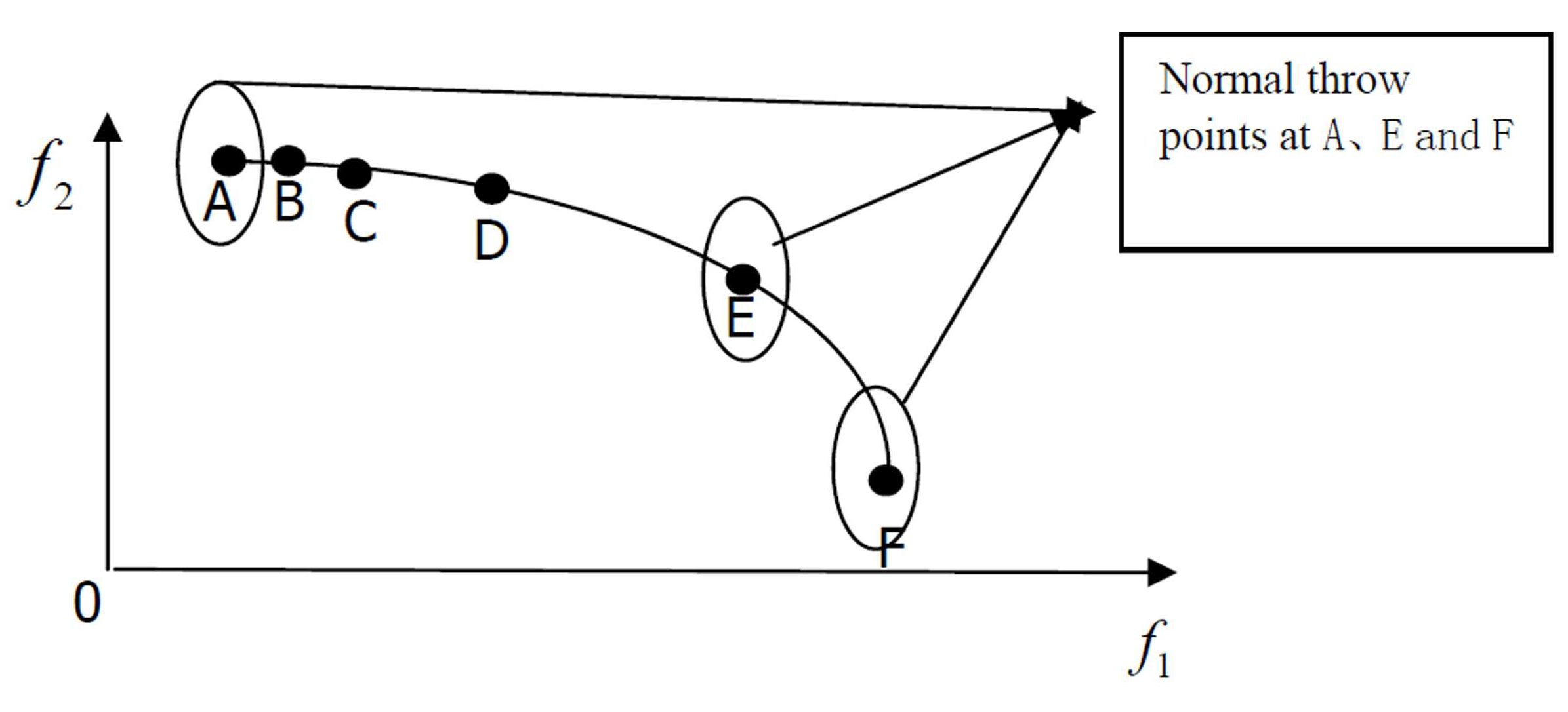
Step 1: Identify a sparse solution based on the crowding entropy, as shown in Figure 1.

Step 2: In the decision space, $A⟶x_A$, $E⟶x_E$, and $F⟶x_F$. We normally throw h points based on centres $x_A$, $x_E$, and $x_F$ and variance $\sigma$. The random variable $Z\sim N(A,\sigma )$, and we add h random points to the TPS. It should be noted that the value of the variance $\sigma$ is $\frac{1}{5}$ the width of each dimension. For example; $x=(x_1,x_2)\in [-10,0]\times [0,10]⟹\sigma =\left(\begin{array}{cc}2& 0\\ 0& 2\end{array}\right)$; $h=5$.

2. Throw points into the current population to produce a Gaussian mutation points set (GMPS).

The algorithm chooses R solutions based on the prescribed probability in the current population, and normal throw points are established at R solutions (method based on (i): Step 2). Finally, we obtain a new GMPS.

3.2.3. Improved Learning Strategy

The standard PSO algorithm is used to solve the single-objective optimization problem, therefore, it is difficult to select the $g_{\mathrm{best}}$ value of velocity and update the formula for MOPs. The reason for this issue is that MOPs do not contain the global optimal solution. In many previous articles, researchers have randomly selected a solution from the external archive as the global optimal solution $g_{\mathrm{best}}$, but this method lacks pertinence and cannot reflect the guidance of $g_{\mathrm{best}}$. Therefore, this article presents a modified velocity formula, redefines the value $g_{\mathrm{best}}$ of Equation (2) and more efficiently applies $g_{\mathrm{best}}$ to solve MOPs.

(i) When $x_i^T$ is not in the external archive, all solutions in the archive that dominate $x_i^T$ can be regarded as global optimal solutions. Therefore, we provide a linear combination of these solutions.

Suppose that there are k archive solutions that dominate $x_i^T:a_1^T,a_2^T,\cdots ,a_k^T$. A set of weights $w_j$ is randomly generated, where $j=1,2,\cdots ,k$ and ${\displaystyle \sum _{j=1}^k}{w}_j=1$. Thus, $g_{\mathrm{best}}$ can be expressed as follows:

$$g_{\mathrm{best}}=\sum _{j=1}^k{w}_j{a}_j^T.$$

Velocity is updated in the formula as follows:

$$v_{id}^{T+1}=w{v}_{id}^T+c_1{r}_1(p_{i\mathrm{best}d}-x_{id}^T)+c_2{r}_2(g_{\mathrm{best}d}-x_{id}^T).$$

(5)

(ii) When $x_i^T$ is in the external archive, the concept of a global optimal solution is meaningless for $x_i^T$ because the global optimal solution is a non-dominated solution. Therefore, all other solutions cannot be better than this solution, and $g_{\mathrm{best}}$ does not exist. Hence, the three parts of Equation (2) are unnecessary, and the velocity updating formula is as follows:

$$v_{id}^{T+1}=w{v}_{id}^T+c_1{r}_1(p_{i\mathrm{best}d}-x_{id}^T).$$

(6)

The position update formula still uses the original model: $x_{id}^{T+1}=x_{id}^T+v_{id}^{T+1}$.

3.2.4. Update External Archive

The updating process of the external archive is an important problem for MOPs. Researchers typically use the archive update rules to compare the current population and the old external archive and then generate a new external archive to further improve the performance of the external archive. This paper uses three sets to update the old external archive. The specific updating methods are shown in Figure 2.

3.2.5. Population Elitist Incremental Strategy

To increase the convergence rate of the population when the algorithm generates the offspring population, we consider the effect of not only the parent population but also the external archive. This paper proposes an elitist incremental strategy that increases the number of external archive solutions in the offspring population to form a new offspring population. The definition is as follows:

$$\begin{array}{cc}& \mathrm{A} \mathrm{new} \mathrm{offspring} \mathrm{population}\hfill \\ \hfill =& \mathrm{randomly} \mathrm{selected}(N-L)\mathrm{offspring} \mathrm{solutions}\hfill \\ & +\mathrm{randomly} \mathrm{selected}L\mathrm{external} \mathrm{archive} \mathrm{solutions},\hfill \end{array}$$

(7)

where N is the population size,

$$L=\left\{\begin{array}{cc}T\hfill & T\le \left[\frac{N}{2}\right]\&\left|A\right|\ge T\hfill \\ \left|A\right|\hfill & T\le \left[\frac{N}{2}\right]\&\left|A\right|<T\hfill \\ \left[\frac{N}{2}\right]\hfill & T>\left[\frac{N}{2}\right]\&\left|A\right|\ge \left[\frac{N}{2}\right]\hfill \\ \left|A\right|\hfill & T>\left[\frac{N}{2}\right]\&\left|A\right|<\left[\frac{N}{2}\right]\hfill \end{array}\right.,$$

T is the number of iterations, and $\left|A\right|$ is the external archive of size A at iteration T.

As a result, the population has strong exploration abilities and can find a wider range of non-dominated solutions at the early stage. The population will further explore the known non-dominated solutions and move closer to the true Pareto front in the later stage.

4. Overview of the MOIPSO Algorithm

As previously discussed, the MOIPSO algorithm can be summarized as follows.

Step l: Randomly initialize the position and velocity of each particle within the search space.

(a) Set the following parameters; $c_1=c_2$, $v_{\max }$, $v_{\min }$, $w_{\max }$, $w_{\min }$, $T=0$, the Gaussian mutation probability $p_r$, the maximum generation number $T_{\max }$, the population size N, and the maximum external archive size $A_{\max }$.

(b) Randomly initialize the population and the velocity.

Step 2: Calculate the fitness of the particles in the initialized population, and initialize the optimal position $p_{i\mathrm{best}}$ of the i-th particle.

Step 3: Initialize an update to the external archive A.

Step 4: For $T=1$:

(a) Renew the velocities of particles based on Equations (5) and (6) and the position of particles based on Equation (7) to form the middle population;

(b) Select the particles based on the Gaussian mutation probability $p_r$ and throw points using the Gaussian mutation strategy (ii) to produce a GMPS;

(c) Calculate the crowding entropy of the external archive solutions and throw points based on the Gaussian mutation strategy (i) to produce a TPS;

(d) Renew the external archive A based on Section 3.2.4. If $\left|A\right|>A_{\max }$, then delete the most crowded particles according to the crowding entropy;

(f) Renew the middle population using the elitist incremental strategy, and form the new offspring population;

(g) Calculate the fitness of the particle in the offspring population;

(h) Renew the optimal position $p_{i\mathrm{best}}$ of each particle;

(i) If the termination criterion is satisfied, then output the Pareto optimal solutions. Otherwise, let $T=T+1$ and go to Step (a).

5. Methods and Simulation Experiments

5.1. Test Problems

To test the performance of MOIPSO, eight unconstrained optimization problems were used in the experiments. The SCH, KUR, and FON functions were suggested by Schaffer in 1985 [25], Kursawe in 1991 [26], and Fonseca in 1998 [27], respectively. The remainders are ZDT problems suggested by Zitzler et al. in 2000 [28]. The optimization problems are described in

Table 1. The tested optimization problems.

Function	Objective Functions	D	Variable Bounds	Characteristics of the Pareto Front
SCH	$\left\{\begin{array}{c}{f}_1(x)=x^2\hfill \\ f_2(x)={(x-2)}^2\hfill \end{array}\right.$	1	$x\in [-{10}^3,{10}^3]$	Convex
FON	$\left\{\begin{array}{c}{f}_1(x)=1-exp(-{\displaystyle \sum _{i=1}^3}{(x_i-\frac{1}{\sqrt{3}})}^2)\hfill \\ f_2(x)=1-exp(-{\displaystyle \sum _{i=1}^3}{(x_i+\frac{1}{\sqrt{3}})}^2)\hfill \end{array}\right.$	3	$x_i\in [-4,4]$	Nonconvex
KUR	$\left\{\begin{array}{c}{f}_1(x)={\displaystyle \sum _{i=1}^{n-1}}(-10exp(-0.2\sqrt{{x_i}^2+{x_{i+1}}^2}))\hfill \\ f_2(x)={\displaystyle \sum _{i=1}^n}({\left|x_i\right|}^{0.8}+5sin({x_i}^3))\hfill \end{array}\right.$	3	$x_i\in [-5,5]$	Disconnect
ZDT1	$\left\{\begin{array}{c}{f}_1(x)=x_1\hfill \\ f_2(x)=g(x)[1-\sqrt{x_1/g(x)}]\hfill \\ g(x)=1+9({\displaystyle \sum _{i=2}^n}{x}_i)/(n-1)\hfill \end{array}\right.$	30	$x_i\in [0,1]$	Convex
ZDT2	$\left\{\begin{array}{c}{f}_1(x)=x_1\hfill \\ f_2(x)=g(x)[1-{(x_1/g(x))}^2]\hfill \\ g(x)=1+9({\displaystyle \sum _{i=2}^n}{x}_i)/(n-1)\hfill \end{array}\right.$	30	$x_i\in [0,1]$	Nonconvex
ZDT3	$\left\{\begin{array}{c}{f}_1(x)=x_1\hfill \\ f_2(x)=g(x)(1-\sqrt{x_1/g(x)}-x_{1}sin(10\pi x_1)/g(x))\hfill \\ g(x)=1+9{\displaystyle \sum _{i=2}^n}{x}_i/(n-1)\hfill \end{array}\right.$	30	$x_i\in [0,1]$	Convex disconnect
ZDT4	$\left\{\begin{array}{c}{f}_1(x)=x_1\hfill \\ f_2(x)=g(x)(1-\sqrt{x_1/g(x)})\hfill \\ g(x)=1+10(n-1)+{\displaystyle \sum _{i=2}^n}[{x_i}^2-10cos(4\pi x_i)]\hfill \end{array}\right.$	10	$x_1\in [0,1]$	Nonconvex
			$x_i\in [-5,5]$ $i=2,\cdots ,n$
ZDT6	$\left\{\begin{array}{c}{f}_1(x)=1-exp(-4x_1){sin}^6(6\pi x_1)\hfill \\ f_2(x)=g(x)[1-{(f_1(x)/g(x))}^2]\hfill \\ g(x)=1+9{\left[{\displaystyle \sum _{i=2}^n}{x}_i/(n-1)\right]}^{0.25}\hfill \end{array}\right.$	10	$x_i\in [0,1]$	Nonconvex

.

5.2. Performance Measures

The standard performance measures of multi-objective evolutionary algorithms were used to evaluate the performance of the proposed algorithm. The performance measures are briefly described as follows.

5.2.1. Convergence Measure Indicator

Ideally, the iterative process of MOEA approaches the Pareto front, but in most cases, it is difficult to find the true Pareto front. The proximity of the approximate solutions to the Pareto optimal solutions is a main indicator.

The concept of generational distance was introduced by Van Veldhuizen [29] to measure the proximity of the approximate solutions to the Pareto optimal solutions. This indicator is defined as follows:

$$GD=\frac{\sqrt{{\displaystyle \sum _{i=1}^n}{\mathrm{dist}}_i^2}}{n},$$

(8)

where n is the number of non-dominated solutions. When the Pareto fronts of the objective function can be expressed in analytic form, ${\mathrm{dist}}_i$ is measured by the Euclidean distance (in objective space) between the i-th non-dominated solution and the nearest member of the Pareto optimal set. Otherwise, ${\mathrm{dist}}_i$ is measured by the Euclidean distance between the i-th non-dominated solution and the reference point set. It is clear that a smaller value of $GD$ is better, and $GD=0$ indicates that the non-dominated solution set is located in the true Pareto front.

5.2.2. Distribution Measure Indicator

Typically, we hope that non-dominated solutions are uniformly distributed in the true Pareto front. Two main factors used to measure the distribution are uniformity and width:

(1) Distribution uniformity ($\Delta$)

The indicator $\Delta$ [4] is used to measure the uniformity and diversity of the non-dominated solution set. When calculating this indicator, we must sort the obtained non-dominated solutions based on the specified objective function values. This indicator is defined as follows:

$$\Delta =\frac{h_f+h_l+{\displaystyle \sum _{i=1}^{n-1}}|h_i-\overline{h}|}{h_f+h_l+(n-1)\overline{h}},$$

(9)

where n is the number of non-dominated solutions, $h_i$ is the Euclidean distance between neighbouring solutions in the non-dominated solution set, $\overline{h}$ is the mean of all $h_i$ values, $h_f$ and $h_l$ are the Euclidean distances between the extreme solutions of the Pareto optimal solution set and the boundary solutions of the non-dominated solution set. When the non-dominated solution set is uniformly distributed in the true Pareto front, $h_f=0$, $h_l=0$, and all $h_i=\overline{h}$, therefore, $\Delta =0$. A small value of $\Delta$ indicates better uniformity in the true Pareto front.

(2) Distribution width ($\mathit{DW}$)

Generally, it is favourable if the boundary solutions can be included in the non-dominated solution set. In other words, in these types of problems, researchers hope to find the boundary points of the true Pareto fronts.

The indicator $M_3^{*}(NP)$, which measures the distribution width, was proposed by Zitzler et al. [28]. The associated formula is as follows:

$$M_3^{*}(NP)=\sqrt{\sum _{i=1}^M\max \{\parallel p_i-q_i{\parallel }^{*},p,q\in NP\}},$$

(10)

where $NP$ is the non-dominated solution set and M is the dimension of the non-dominated solutions. Notably, $M_3^{*}$ can measure the distribution width of the non-dominated solution set, but when the distribution range of the Pareto front is too large or the dimensions of the solutions are large, the value of $M_3^{*}$ will be large. Therefore, it is difficult to compare and compile the data.

Based on the aforementioned method, the new indicator, $DW$, is provided. The concrete form of this indicator is as follows:

$$DW=\left|\frac{{\displaystyle \prod _{i=1}^M}\max \left\{\right|p_i-q_i|,p,q\in NP\}}{{\displaystyle \prod _{i=1}^M}\max \left\{\right|p_i^{\prime }-q_i^{\prime }|,p^{\prime },q^{\prime }\in RP\}}-1\right|,$$

(11)

where $RP$ is the Pareto optimal set or the reference point set. Notably, a small value of $DW$ reflects a better distribution uniformity for the non-dominated solution set.

5.3. Algorithm Comparison

To validate the MOIPSO algorithm, we compared it to NSGA-II [4] and MOPSO [7] based on the above three performance measures. The source codes of NSGA-II and MOPSO are available at http://delta.cs.cinvestav.mx/~ccoello/EMOO/ (matlab code).

The initial population size is 100 for MOIPSO, NSGA-II and MOPSO. The number of iterations directly affects the time complexity of the algorithm, and the convergence of the problem with different iterations is discussed [30]. It can be found that when the program reaches a stable state, the subsequent iterations can no longer improve the performance of the algorithm, but only increase the running time. Therefore, through a large number of numerical experiments, different iteration numbers were chosen based on the complexity of the problems in the three algorithms. The number of iterations completed was 60 for SCH, 100 for FON and KUR, 300 for ZDT1, ZDT2, and ZDT3, and 1000 for ZDT4 and ZDT6.

The range of the parameter has been discussed in some literature [31], so we took the commonly used parameter values for NSGAII and MOPSO. To make the test and its results more comparable, for MOIPSO, the same parameters as MOPSO took the same values, and other parameters were set after a large number of numerical experiments. In the MOPSO and MOIPSO algorithms, $c_1=c_2=1.7$, while $r_1$ and $r_1$ are assigned random values between 0 and 1. In MOPSO, the inertia weight is $w=0.7$, and the inertia weight damping ratio $w_{damp}=1$. In MOIPSO, the inertia weight w adaptively decreased from $w_{\max }=0.9$ to $w_{\min }=0.4$ according to the following formula: $w=w_{\max }-\frac{T(w_{\max }-w_{\min })}{T_{\max }}$. In the NSGA-II [4] algorithm, the crossover probability is $0.8$, and the mutation probability is $0.3$. To evaluate the statistical performance, all the experiments are run 30 times. The best, worst, mean, and average deviations are shown in

Table 2. Comparison of the results of multi-objective improved particle swarm optimization algorithm (MOIPSO) and different algorithms based on the indicator, $GD$.

Function	Statistic	MOPSO	NSGA-II	MOIPSO
SCH	Best	$8.72\times {10}^{-4}$	$8.37\times {10}^{-4}$	$8.34\times {10}^{-4}$
	Worst	$1.30\times {10}^{-3}$	$1.10\times {10}^{-3}$	$1.00\times {10}^{-3}$
	Mean	$9.66\times {10}^{-4}$	$9.56\times {10}^{-4}$	$9.41\times {10}^{-4}$
	Std	$7.89\times {10}^{-5}$	$4.70\times {10}^{-5}$	$4.76\times {10}^{-5}$
FON	Best	$1.00\times {10}^{-3}$	$1.10\times {10}^{-3}$	$1.00\times {10}^{-3}$
	Worst	$1.30\times {10}^{-3}$	$1.30\times {10}^{-3}$	$1.20\times {10}^{-3}$
	Mean	$1.10\times {10}^{-3}$	$1.20\times {10}^{-3}$	$1.10\times {10}^{-3}$
	Std	$6.22\times {10}^{-5}$	$3.73\times {10}^{-5}$	$6.08\times {10}^{-5}$
KUR	Best	$3.10\times {10}^{-3}$	$1.60\times {10}^{-3}$	$1.40\times {10}^{-3}$
	Worst	$3.09\times {10}^{-2}$	$4.40\times {10}^{-3}$	$3.80\times {10}^{-3}$
	Mean	$5.80\times {10}^{-3}$	$3.00\times {10}^{-3}$	$2.50\times {10}^{-3}$
	Std	$4.82\times {10}^{-3}$	$6.43\times {10}^{-4}$	$4.13\times {10}^{-4}$
ZDT1	Best	$1.70\times {10}^{-3}$	$1.96\times {10}^{-2}$	$5.91\times {10}^{-4}$
	Worst	$6.43\times {10}^{-2}$	$5.49\times {10}^{-2}$	$3.20\times {10}^{-3}$
	Mean	$2.63\times {10}^{-2}$	$3.03\times {10}^{-2}$	$1.00\times {10}^{-3}$
	Std	$1.81\times {10}^{-2}$	$7.80\times {10}^{-3}$	$6.30\times {10}^{-4}$
ZDT2	Best	$5.28\times {10}^{-5}$	$2.96\times {10}^{-2}$	$3.51\times {10}^{-4}$
	Worst	$1.55\times {10}^{-1}$	$4.99\times {10}^{-2}$	$3.10\times {10}^{-3}$
	Mean	$4.19\times {10}^{-2}$	$3.84\times {10}^{-2}$	$7.52\times {10}^{-4}$
	Std	$4.49\times {10}^{-2}$	$5.40\times {10}^{-3}$	$5.94\times {10}^{-4}$
ZDT3	Best	$4.04\times {10}^{-4}$	$2.19\times {10}^{-2}$	$5.01\times {10}^{-4}$
	Worst	$1.08\times {10}^{-1}$	$4.74\times {10}^{-2}$	$7.10\times {10}^{-3}$
	Mean	$3.82\times {10}^{-2}$	$3.30\times {10}^{-2}$	$1.20\times {10}^{-3}$
	Std	$3.27\times {10}^{-2}$	$8.10\times {10}^{-3}$	1.50$\times {10}^{-3}$
ZDT4	Best	$1.10\times {10}^{-1}$	$1.30\times {10}^{-3}$	$3.23\times {10}^{-4}$
	Worst	$2.01\times {10}^{-1}$	$2.86\times {10}^{-2}$	$1.61\times {10}^{-2}$
	Mean	$1.40\times {10}^{-1}$	$4.90\times {10}^{-3}$	$9.90\times {10}^{-3}$
	Std	$1.67\times {10}^{-2}$	$6.20\times {10}^{-3}$	$2.37\times {10}^{-2}$
ZDT6	Best	$2.72\times {10}^{-4}$	$1.19\times {10}^{-1}$	$5.36\times {10}^{-4}$
	Worst	$3.32\times {10}^{-1}$	$1.65\times {10}^{-1}$	$4.38\times {10}^{-2}$
	Mean	$2.29\times {10}^{-2}$	$1.46\times {10}^{-1}$	$1.09\times {10}^{-2}$
	Std	$5.96\times {10}^{-2}$	$9.10\times {10}^{-3}$	$1.13\times {10}^{-2}$

,

Table 3. Comparison of the results of MOIPSO and different algorithms based on $\Delta$.

Function	Statistic	MOPSO	NSGA-II	MOIPSO
SCH	Best	$4.68\times {10}^{-1}$	$4.68\times {10}^{-1}$	$4.67\times {10}^{-1}$
	Worst	$4.80\times {10}^{-1}$	$4.73\times {10}^{-1}$	$4.70\times {10}^{-1}$
	Mean	$4.68\times {10}^{-1}$	$4.69\times {10}^{-1}$	$4.67\times {10}^{-1}$
	Std	$2.80\times {10}^{-3}$	$1.70\times {10}^{-3}$	$4.53\times {10}^{-4}$
FON	Best	$4.82\times {10}^{-1}$	$4.81\times {10}^{-1}$	$4.84\times {10}^{-1}$
	Worst	$4.94\times {10}^{-1}$	$4.95\times {10}^{-1}$	$4.85\times {10}^{-1}$
	Mean	$4.86\times {10}^{-1}$	$4.87\times {10}^{-1}$	$4.85\times {10}^{-1}$
	Std	$2.60\times {10}^{-3}$	$3.90\times {10}^{-3}$	$4.70\times {10}^{-4}$
KUR	Best	$4.59\times {10}^{-1}$	$4.64\times {10}^{-1}$	$4.63\times {10}^{-1}$
	Worst	$4.69\times {10}^{-1}$	$4.69\times {10}^{-1}$	$4.68\times {10}^{-1}$
	Mean	$4.63\times {10}^{-1}$	$4.67\times {10}^{-1}$	$4.66\times {10}^{-1}$
	Std	$2.10\times {10}^{-3}$	$1.30\times {10}^{-3}$	$1.10\times {10}^{-3}$
ZDT1	Best	$4.08\times {10}^{-2}$	$2.67\times {10}^{-1}$	$1.13\times {10}^{-2}$
	Worst	$3.54\times {10}^{-1}$	$4.05\times {10}^{-1}$	$1.08\times {10}^{-1}$
	Mean	$2.47\times {10}^{-1}$	$3.43\times {10}^{-1}$	$4.28\times {10}^{-2}$
	Std	$8.62\times {10}^{-2}$	$3.71\times {10}^{-2}$	$9.70\times {10}^{-3}$
ZDT2	Best	$3.78\times {10}^{-1}$	$4.09\times {10}^{-1}$	$3.90\times {10}^{-3}$
	Worst	$9.92\times {10}^{-1}$	$4.90\times {10}^{-1}$	$1.47\times {10}^{-1}$
	Mean	$6.88\times {10}^{-1}$	$4.59\times {10}^{-1}$	$2.65\times {10}^{-2}$
	Std	$1.54\times {10}^{-1}$	$1.99\times {10}^{-2}$	$3.17\times {10}^{-2}$
ZDT3	Best	$4.19\times {10}^{-1}$	$2.64\times {10}^{-1}$	$2.50\times {10}^{-3}$
	Worst	$7.06\times {10}^{-1}$	$3.60\times {10}^{-1}$	$1.94\times {10}^{-1}$
	Mean	$5.58\times {10}^{-1}$	$3.13\times {10}^{-1}$	$3.08\times {10}^{-2}$
	Std	$6.58\times {10}^{-2}$	$2.94\times {10}^{-2}$	$4.57\times {10}^{-2}$
ZDT4	Best	$6.11\times {10}^{-1}$	$1.33\times {10}^{-2}$	$3.70\times {10}^{-3}$
	Worst	$6.89\times {10}^{-1}$	$3.50\times {10}^{-1}$	$4.74\times {10}^{-1}$
	Mean	$6.50\times {10}^{-1}$	$8.96\times {10}^{-2}$	$8.88\times {10}^{-2}$
	Std	$1.95\times {10}^{-2}$	$9.90\times {10}^{-2}$	$1.50\times {10}^{-1}$
ZDT6	Best	$1.07\times {10}^{-2}$	$4.86\times {10}^{-1}$	$1.11\times {10}^{-2}$
	Worst	$4.52\times {10}^{-1}$	$7.95\times {10}^{-1}$	$4.08\times {10}^{-1}$
	Mean	$2.43\times {10}^{-1}$	$6.29\times {10}^{-1}$	$2.28\times {10}^{-1}$
	Std	$1.28\times {10}^{-1}$	$6.92\times {10}^{-2}$	$1.28\times {10}^{-1}$

and

Table 4. Comparison of the results of MOIPSO and different algorithms based on $DW$.

Function	Statistic	MOPSO	NSGA-II	MOIPSO
SCH	Best	$1.00\times {10}^{-3}$	$4.46\times {10}^{-5}$	$4.44\times {10}^{-5}$
	Worst	$6.43\times {10}^{-2}$	$4.35\times {10}^{-2}$	$1.80\times {10}^{-2}$
	Mean	$1.43\times {10}^{-2}$	$1.66\times {10}^{-2}$	$2.70\times {10}^{-3}$
	Std	$1.56\times {10}^{-2}$	$1.26\times {10}^{-2}$	$3.70\times {10}^{-3}$
FON	Best	$2.62\times {10}^{-4}$	$4.21\times {10}^{-4}$	$1.90\times {10}^{-3}$
	Worst	$3.36\times {10}^{-2}$	$9.09\times {10}^{-2}$	$8.00\times {10}^{-3}$
	Mean	$9.60\times {10}^{-3}$	$3.10\times {10}^{-2}$	$5.50\times {10}^{-3}$
	Std	$9.30\times {10}^{-3}$	$2.19\times {10}^{-2}$	$1.60\times {10}^{-3}$
KUR	Best	$3.07\times {10}^{-4}$	$5.50\times {10}^{-3}$	$2.40\times {10}^{-4}$
	Worst	$7.55\times {10}^{-2}$	$7.36\times {10}^{-2}$	$1.11\times {10}^{-2}$
	Mean	$1.32\times {10}^{-2}$	$3.71\times {10}^{-2}$	$3.30\times {10}^{-3}$
	Std	$1.82\times {10}^{-2}$	$1.95\times {10}^{-2}$	$2.40\times {10}^{-3}$
ZDT1	Best	$7.80\times {10}^{-3}$	$5.00\times {10}^{-2}$	$3.20\times {10}^{-3}$
	Worst	$1.33$	$1.29$	$2.26\times {10}^{-2}$
	Mean	$5.23\times {10}^{-1}$	$4.98\times {10}^{-1}$	$1.17\times {10}^{-2}$
	Std	$4.05\times {10}^{-1}$	$2.83\times {10}^{-1}$	$6.20\times {10}^{-2}$
ZDT2	Best	$1.54\times {10}^{-1}$	$1.60\times {10}^{-3}$	$3.30\times {10}^{-3}$
	Worst	$1.00$	$6.40\times {10}^{-1}$	$2.99\times {10}^{-1}$
	Mean	$7.72\times {10}^{-1}$	$2.07\times {10}^{-1}$	$4.16\times {10}^{-2}$
	Std	$2.55\times {10}^{-1}$	$1.49\times {10}^{-1}$	$6.28\times {10}^{-2}$
ZDT3	Best	$4.60\times {10}^{-3}$	$3.49\times {10}^{-2}$	$1.83\times {10}^{-4}$
	Worst	$8.93\times {10}^{-1}$	$5.54\times {10}^{-1}$	$9.63\times {10}^{-1}$
	Mean	$6.23\times {10}^{-1}$	$2.59\times {10}^{-1}$	$8.52\times {10}^{-2}$
	Std	$2.37\times {10}^{-1}$	$1.54\times {10}^{-1}$	$2.37\times {10}^{-1}$
ZDT4	Best	$1.92\times {10}^{-1}$	$9.28\times {10}^{-4}$	$6.50\times {10}^{-3}$
	Worst	$1.00$	$1.64$	$1.68$
	Mean	$6.33\times {10}^{-1}$	$2.21\times {10}^{-1}$	$2.07\times {10}^{-1}$
	Std	$1.95\times {10}^{-1}$	$4.03\times {10}^{-1}$	$1.55\times {10}^{-1}$
ZDT6	Best	$1.42\times {10}^{-2}$	$1.04\times {10}^{-2}$	$2.20\times {10}^{-4}$
	Worst	$6.87$	$1.17$	$1.09$
	Mean	$1.18$	$2.78\times {10}^{-1}$	$1.86\times {10}^{-1}$
	Std	$1.48$	$2.78\times {10}^{-1}$	$8.77\times {10}^{-1}$

, respectively.

The $GD$ results are shown in Table 2. MOIPSO exhibits the best $GD$ values for SCH, KUR, ZDT1 and ZDT4. MOPSO displays the best $GD$ values for ZDT2, ZDT3, and ZDT6. FON, MOIPSO, and MOPSO exhibit similar results. For the worst $GD$, MOIPSO displays high stability and consistently yields the lowest worst $GD$ value in all test problems. For the mean $GD$, MOIPSO produces the best mean values for all test problems except ZDT4, for which FON, MOIPSO, and MOPSO exhibit similar results. With respect to the standard deviation of $GD$, MOIPSO exhibits the best solution for KUR, ZDT1, ZDT2, and ZDT3. NSGA-II yields the best results for the other functions. Thus, MOIPSO produces better values of $GD$ indicators than the other two algorithms in most test problems, and the results of MOIPSO are better than those of the other algorithms by 1∼2 orders of magnitude. This finding indicates that the resulting Pareto fronts obtained via MOIPSO are closer to the true Pareto fronts, and MOIPSO can effectively improve convergence.

Some information for $\Delta$ is shown in Table 3. For the SCH and ZDT1 functions, all the solutions of MOIPSO are better than those of the other algorithms. MOPSO exhibits the best, and the mean best, $\Delta$ value for KUR. MOIPSO has the minimal worst $\Delta$ and the best standard deviation. MOIPSO has the best, the mean best, and the minimal worst $\Delta$ values for ZDT2 and ZDT3, but the standard deviation of NSGA-II is the best. MOIPSO displays the best and the mean best $\Delta$ values for ZDT4. NSGA-II exhibits the minimal worst $\Delta$, and MOPSO yields the best standard deviation. MOPSO provides the best $\Delta$ for ZDT6. MOIPSO has the minimal worst $\Delta$ and the mean best $\Delta$, and the minimal standard deviation of NSGA-II is the best. Table 3 shows that MOIPSO provides the best mean solution for all seven functions. Therefore, the MOIPSO results are evenly distributed in the experiments, however, they are not shown for all the functions.

Table 4 shows the results of a new quality indicator—$DW$. All the solutions of MOIPSO are better than those of the other algorithms for SCH, KUR, and ZDT1. MOIPSO yields the three best indicators for the FON function, and MOPSO provides the best solution for $DW$. NSGA-II exhibits the best $DW$ solution for ZDT2, and the other indicators of MOIPSO are the best. MOIPSO displays the best and the mean best $DW$ for ZDT3, and NSGA-II yields the minimal worst $DW$ and the best standard deviation. NSGA-II exhibits the best $DW$ for ZDT4, and MOPSO displays the minimal worst $DW$. MOIPSO produces the mean best $DW$ and the minimal standard deviation. For the ZDT6 function, NSGA-II exhibits the minimal standard deviation, and the other indicators of MOIPSO are the best. Similarly, the $DW$ results in Table 4 show that MOIPSO is able to produce the best distribution of solutions in the Pareto optimal front for most of the test functions.

According to the above statistical analyses, MOIPSO successfully solves the SCH, ZDT1 and ZDT6 problems, as illustrated by Figure 3, Figure 4 and Figure 5. Figure 3 shows that the three algorithms have similar convergence performances for the SCH function, however, MOIPSO exhibits better uniformity. Figure 4 and Figure 5 illustrate the superior convergence and distribution results of MOIPSO compared with those of the other algorithms. Furthermore, by combining the data from Table 4 and the figures, we can see that when the boundary solutions do not exist in non-dominated solutions or solutions do not converge to the true Pareto front, then the $DW$ value is very large. In the case of NSGAII and MOPSO for ZDT6, because some points are far away from the true optimal pare fronts, their $DW$ values are ${10}^{-2}$, but the values are ${10}^{-4}$ for MOIPSO and we can find that all the solutions are near the true optimal Pareto fronts in Figure 4. Thus, the $DW$ indicator can measure the distribution width of the non-dominated solution set.

From the numerical results, we can also see that the MOIPSO algorithm performs better than other algorithms in distribution uniformity and width. This is obviously a good result of the Gaussian mutation throw point strategy. However, this method is not omnipotent. Firstly, when the number of throwing points is too large, the running time will rapidly increase. It is difficult to determine the number, so in this paper, we have done a lot of experiments to determine it. Secondly, for all sparse solutions, we will throw points, so when the Pareto optimal front of optimization problem is very complex and contains a large number of outliers, the effectiveness of our Gaussian mutation throw point strategy will be affected.

6. Conclusions

A new multi-objective PSO algorithm based on Gaussian mutation and an improved learning strategy (MOIPSO) is presented to solve MOPs. First, MOIPSO builds different learning strategies to update the individual positions of the non-dominated and dominated solutions. Then, the Gaussian mutation strategy is used to create throw points at sparse and boundary positions. These updating strategies yield high convergence and a satisfactory distribution. To further measure the distribution width, the indicator $DW$ is proposed.

The performance of MOIPSO was tested based on different MOP benchmark functions with convex and nonconvex objection functions. To demonstrate the effectiveness of MOIPSO, the results were compared to those of MOPSO and NSGA-II. The experimental results showed that MOIPSO significantly outperforms all other algorithms based on the test problems with respect to three metrics. The resulting data and figures indicate that the proposed $DW$ indicator is reasonable.

In this article, only two-objective functions are tested. In the near future, we also plan to evaluate MOIPSO using other objective test functions. Furthermore, most parameters in this paper (such as the number of throw points, cognitive coefficient, etc.) have certain values. It would be interesting to study whether these control parameters could adaptively change as the iteration time increases.

References

- Miettinen, K.M. Nonlinear Multi-Objective Optimization; Kluwer Academic Publishers: Boston, MA, USA, 1999. [Google Scholar]
- Deb, K. Multi-Objective Optimization Using Evolutionary Algorithms; John Wiley and Sons: Hoboken, NJ, USA, 2001. [Google Scholar]
- Fonseca, C.M.; Fleming, P.J. Genetic Algorithm for Multi-Objective Optimization: Formulation, Discussion and Generalization; Morgan Kaufmann Publishers: Burlington, MA, USA, 1993. [Google Scholar]
- Deb, K.; Pratap, A.; Agrawal, S.; Meyarivan, T. A fast and elitist multi-objective genetic algorithm: NSGA-II. IEEE Trans. Evol. Comput. 2002, 6, 182–197. [Google Scholar] [CrossRef]
- Zitzler, E.; Thiele, L. Multi-objective evolutionary algorithms: A comparative case study and the strength pareto approach. IEEE Trans. Evol. Comput. 1999, 3, 257–271. [Google Scholar] [CrossRef]
- Knowles, J.D.; Corne, D.W. Approximating the nondominated front using the Pareto archived evolution strategy. IEEE Trans. Evol. Comput. 2000, 8, 149–172. [Google Scholar] [CrossRef]
- Coello, C.A.C.; Pultdo, G.T.; Lechuga, M.S. Handling multiple objectives with particle swarm optimization. IEEE Trans. Evol. Comput. 2004, 8, 256–279. [Google Scholar] [CrossRef]
- Sierra, M.R.; Coello, C.A.C. Improving PSO-Based Multi-Objective Optimization Using Crowding, Mutation and ε-Dominance; Springer: Berlin/Heidelberg, Germany, 2005; pp. 505–519. [Google Scholar]
- Reddy, M.J.; Kumar, D.N. An efficient multi-objective optimization algorithm based on swarm intelligence for engineering design. Eng. Optim. 2007, 39, 49–68. [Google Scholar] [CrossRef]
- Leong, W.F.; Yen, G.G. PSO-based multi-objective optimization with dynamic population size and adaptive local archives. IEEE Trans. Syst. Man Cybern. Part B 2008, 38, 1270–1293. [Google Scholar] [CrossRef] [PubMed]
- Yen, G.G.; Leong, W.F. Dynamic multiple swarms in multi-objective particle swarm optimization. IEEE Trans. Syst. Man Cybern. Part B 2009, 39, 890–911. [Google Scholar] [CrossRef]
- Chen, D.B.; Zou, F.; Wang, J.T. A multi-objective endocrine PSO algorithm and application. Appl. Soft Comput. 2011, 11, 4508–4520. [Google Scholar] [CrossRef]
- Lin, Q.; Li, J.; Du, Z.; Chen, J.; Ming, Z. A novel multi-objective particle swarm optimization with multiple search strategies. Eur. J. Oper. Res. 2015, 247, 732–744. [Google Scholar] [CrossRef]
- Meza, J.; Espitia, H.; Montenegro, C.; Giménez, E.; González-Crespo, R. Movpso: Vortex multi-objective particle swarm optimization. Appl. Soft Comput. 2017, 52, 1042–1057. [Google Scholar] [CrossRef]
- Hu, W.; Yen, G.G. Adaptive multi-objective particle swarm optimization based on parallel cell coordinate system. IEEE Trans. Evol. Comput. 2015, 19, 1–18. [Google Scholar]
- Knight, J.T.; Singer, D.J.; Collette, M.D. Testing of a spreading mechanism to promote diversity in multi-objective particle swarm optimization. IEEE Trans. Evol. Comput. 2015, 16, 279–302. [Google Scholar] [CrossRef]
- Cheng, T.; Chen, M.; Fleming, P.J.; Yang, Z.; Gan, S. A novel hybrid teaching learning based multi-objective particle swarm optimization. Neurocomputing 2017, 222, 11–25. [Google Scholar] [CrossRef]
- Coello, C.A.C. Evolutionary multi-objective optimization: A historical view of the field. IEEE Comput. Intell. Mag. 2006, 1, 28–36. [Google Scholar] [CrossRef]
- Zitzler, E. Evolutionary Algorithm for Multiobjective Optimization: Methods and Application; Swiss Federal Institute of Technology: Zurich, Switzerland, 1999. [Google Scholar]
- Kennedy, J.; Eberhart, R.C. Particle Swarm Optimization. In Proceedings of the IEEE International Conference on Neural Networks, Perth, Australia, 27 November–1 December 1995; pp. 1942–1948. [Google Scholar]
- Wang, Y.N.; Wu, L.H.; Yuan, X.F. Multi-objective self-adaptive differential evolution with elitist archive and crowding entropy-based diversity measure. Soft Comput. 2010, 14, 193–209. [Google Scholar] [CrossRef]
- Higashi, N.; Iba, H. Particle Swarm Optimization with Gaussian Mutation; IEEE: Piscataway, NJ, USA, 2013. [Google Scholar]
- Coelho, L.D.S.; Ayala, V.H.; Alotto, P. A Multiobjective Gaussian Particle Swarm Approach Applied to Electromagnetic Optimization. IEEE Trans. Mag. 2010, 46, 3289–3292. [Google Scholar] [CrossRef]
- Liang, H.M.; Zhang, K.; Yu, H.H. Multi-objective Gaussian particle swarm algorithm optimization based on niche sorting for actuator design. Adv. Mech. Eng. 2015, 7, 1–7. [Google Scholar] [CrossRef]
- Schaffer, J.D. Multiple objective optimization with vector evaluated genetic algorithm. In Proceedings of the 1st International Conference on Genetic Algorithm and Their Applications, Pittsburg, CA, USA, 24–26 July 1985; pp. 93–100. [Google Scholar]
- Kursawe, F. A varant of evolution strategies for vector optimization. In International Conference on Parallel Problem Solving from Nature; Springer: Berlin/Heidelberg, Germany, 1991; pp. 193–197. [Google Scholar]
- Fonseca, C.M.; Fleming, P.J. Multiobjective optimization and multiple constraint handling with evolutionary algorithms, Part II: Application example. IEEE Trans. Syst. Man Cybern. A 1998, 28, 38–47. [Google Scholar] [CrossRef]
- Zitzler, E.; Deb, K.; Thiele, L. Comparison of multi-objective evolutionary algorithms: Empirical results. Evol. Comput. 2000, 8, 173–195. [Google Scholar] [CrossRef]
- Van Veldhuizen, D.A.; Lamont, G.B. Evolutionary computation and convergence to a Pareto front. In Late Breaking Papers at the Genetic Programming 1998 Conference; Standford University: Stanford, CA, USA, 1998; pp. 221–228. [Google Scholar]
- Saraswat, A.; Saini, A. Multi-objective optimal reactive power dispatch considering voltage stability in power systems using HFMOEA. Eng. Appl. Artif. Intell. 2013, 26, 390–404. [Google Scholar] [CrossRef]
- Ding, S.X.; Chen, C.; Xin, B.; Psrdalos, P. A bi-objective load balancing model in a distributed simulation system using NSGA-II and MOPSO approaches. Appl. Soft Comput. 2018, 63, 249–267. [Google Scholar] [CrossRef]
Figure 1.
The selection process of the sparse solution.
Figure 2.
The updating process of the external archive.
Figure 3.
For SCH, the comparisons between the true Pareto front and the best ones obtained by three different algorithms.
Figure 4.
For ZDT1, the comparisons between the true Pareto front and the best ones obtained by three different algorithms.
Figure 5.
For ZDT6, the comparisons between the true Pareto front and the best ones obtained by three different algorithms.