Monarch Butterfly Optimization for Facility Layout Design Based on a Single Loop Material Handling Path


School of Air Transport, Transportation and Logistics, Korea Aerospace University, 76, Hanggonddaehak-ro, Deoyang-gu, Goyang-si, Gyeonggi-do 10540, Korea
*
Author to whom correspondence should be addressed.
Mathematics 2019, 7(2), 154; https://doi.org/10.3390/math7020154
Submission received: 26 December 2018
/
Revised: 30 January 2019
/
Accepted: 31 January 2019
/
Published: 6 February 2019
(This article belongs to the Special Issue Evolutionary Computation)
Abstract
:Facility layout problems (FLPs) are concerned with the non-overlapping arrangement of facilities. The objective of many FLP-based studies is to minimize the total material handling cost between facilities, which are considered as rectangular blocks of given space. However, it is important to integrate a layout design associated with continual material flow when the system uses circulating material handling equipment. The present study proposes approaches to solve the layout design and shortest single loop material handling path. Monarch butterfly optimization (MBO), a recently-announced meta-heuristic algorithm, is applied to determine the layout configuration. A loop construction method is proposed to construct a single loop material handling path for the given layout in every MBO iteration. A slicing tree structure (STS) is used to represent the layout configuration in solution form. A total of 11 instances are tested to evaluate the algorithm’s performance. The proposed approach generates solutions as intended within a reasonable amount of time.
1. Introduction
A facility layout design has significant value to the manufacturing world. From the machine lines to the path of material handling equipment, many factors related to operation efficiency depend on the facility layout design [1]. Because a layout configuration is directly related to the material handling performance in a factory or workspace, researchers have been studying optimal facility layouts with various approaches. In academia, this came to be called the facility layout problem (FLP).
The FLP ranges over an arrangement of blocks in a given area [2]. The blocks, which are regarded as departments, can be machines, workspaces or even buildings. In an FLP, departments that are known in size have to be arranged in a given space without overlapping [3]. For cases where each department has a different size, the term unequal area facility layout problem (UAFLP) has been coined. In this study, we use the acronym FLP to mean UAFLP. Mixed integer programming (MIP) can be used to solve FLPs. However, FLPs are categorized as NP-hard because they encounter many restrictions, including location or aspect ratio limitations. These restrictions prevent FLPs from being solved in a reasonable amount of computational time [4]. Therefore, to solve large-sized problems of generally more than 12 departments, various meta-heuristic approaches have been used [5,6,7,8].
In this study, monarch butterfly optimization (MBO), a relatively new meta-heuristic, is adopted to solve the FLP. Inspired by the monarch butterfly species, MBO mimics the butterfly’s group migration [9]. MBO has a simple concept and parameters relative to other meta-heuristic algorithms. The simple structure of the algorithm facilitates the implementation of complicated expressions of the layout representation in computer code. In addition, several studies have successfully demonstrated MBO’s performance [10,11,12,13,14].
When solving an FLP using meta-heuristics, a layout representation method is necessary to construct the department sequence. Indeed, various heuristic methods concerned with layout representation have been proposed. However, pre-defined layout representations such as the flexible bay structure (FBS) or slicing tree structure (STS) have been widely used to easily represent the layout scheme. When assigning the departments to floor space, the FBS only considers one cutting direction. Therefore, the FBS is relatively easy to apply and takes less computational time. However, the STS allows both the vertical and horizontal directions. While this makes the STS more complicated and adds computational time, it also produces a greater variety of layout configurations that combine two directions than the FBS [6]. Most previous studies dealt with loop-based FLPs by using FBS representation. We adopt the STS to gain greater flexibility in solution space and to obtain better solutions.
To estimate the fitness value of the obtained layout, various evaluation methods can be applied. Typically, a rectilinear distance-based approach is used [15] to evaluate the results. However, in this study, a single loop distance is applied to evaluate the layout. This single loop can be regarded as route-of-path-based material handling equipment such as automated guided vehicles (AGVs) or power and free systems. This kind of measurement can aid the design of certain layouts operated with path-based vehicles. We define a single loop distance as the size of a single loop where the material handling equipment can access all of the departments through the path, and the path is never crossed.
To find a single loop in the obtained layout, the single loop construction method is proposed in this study. Before constructing a single loop, a department-searching procedure is conducted to determine a feasible layout. After searching every adjacent department, the single loop department is determined based on the number of adjacent departments. If there are no more departments to be included, the single loop construction method can be finished, and a single loop is obtained. This process is embedded in every MBO iteration, and single loop size minimization becomes the main objective of the layout design.
This paper proceeds as follows. The research background and the literature review are introduced in Section 2, Section 3 deals with the layout representation method and the adoption of MBO in the FLP. Section 4 defines the MBO approach with respect to the FLP. The computational results of this research and the conclusion are described in Section 5 and Section 6, respectively.
2. Background and Literature Review
According to Kochhar et al. [16], because the importance of facility layout has come to the fore, the FLP has been widely studied. As mentioned, the FLP deals with the placement of departments in a given area without overlapping [17]. Typically, a good facility layout is directly related to the material handling cost. Therefore, the objective function value (OFV), which is used to evaluate the layout configuration, is also related to the movement between departments [18]. Several distance measurements exist, as shown in Figure 1. The rectilinear distance in Figure 1a is composed of the absolute distance between two datum points of the department on both the x and y axis. On the contrary, the Euclidean distance, which is the shortest diagonal distance, can be seen in Figure 1d [19]. The contour distance is described in Figure 1b. In this measurement, the movement between two departments must occur along the adjacent department’s boundary. Figure 1c deals with the single loop distance. As previously defined, all departments should be accessible through a single loop. Therefore, in this case, the single loop distance can be the OFV of the layout.
However, in terms of operating circulating path-based material handling systems, the layout configured for the shortest single loop might be helpful. For instance, the derived single loop path can be regarded as a practically appropriate planned path for vehicle-based systems [20]. In this way, the FLP with the single loop can be an industrial alternative to that of general FLPs that deal with traditional distances between departments. Moreover, the single loop is much simpler than other loop networks because there are no interactions or departments along the path [21].
Two early approaches to the single loop under an FLP were conducted by Tanchoco and Sinriech [22] and Sinriech and Tanchoco [21] in the 1990s. They considered a single loop to be a more effective and cost-saving alternative for material handling equipment operation. In their papers, the optimal single-loop (OSL) guide paths for AGVs were proposed for the single closed loop guide path layout. A valid single loop problem and single loop station location problem were developed by the authors and worked well with the general FLPs. Asef-Vaziri et al. [23] defined an FLP with a single loop as the shortest loop design problem (SLDP) and introduced improved integer linear programming (ILP). To demonstrate its performance, several problems were tested. Subsequently, Ahmadi-Javid and Ramshe [24] corrected the ILP formulation and developed a cutting-plane algorithm to generate reasonable computational results. Over time, other researchers have tried to develop a variety of powerful meta-heuristics to obtain better layout solutions in less computational time. In Yang and Peters’ research [25], a two-step heuristic approach was proposed for an open-field type layout with a single loop path. Their approach combined a space-filling curve with simulated annealing (SA). In the first step, a traditional block layout with a directed loop was solved with the combined heuristic approach. Next, an MIP formulation was solved using the spatial coordinate and orientation location inputs from the first stage. Hojabri et al. [26] suggested a decomposition algorithm for solving a single loop material flow. In the process of finding the solution, all departments were located along a loop and removed randomly from that loop until a feasible loop was found. This proposed algorithm was successful in solving large problems in a short amount of time. Jahandideh et al. [27] introduced a genetic algorithm (GA) to design a unidirectional loop in an FLP by considering the total loaded and empty trips. Asef-Vaziri et al. [28] proposed a single loop-based facility layout design. They used a hybrid GA and noted that the computational time could be effectively reduced even with a large number of departments.
Additional forms of single loop FLPs were studied by other researchers. Chae and Peters [29] used a single loop structure as a department placement guideline and applied SA to search for solutions. Niroomand et al. [30] built on Chae and Peters’ department placement strategy and used a modified migrating birds optimization to find a better layout configuration for a closed loop-based facility layout problem (CLLP). Kang et al. [31] applied the cuckoo search algorithm to a CLLP and showed that the algorithm generated quality solutions for the CLLP. More details about loop-based FLPs can be read in the review papers provided by Asef-Vaziri and Laporte [32] and Asef-Vaziri and Kazemi [20].
To solve FLPs using various meta-heuristic approaches, a proper layout representation should be encoded to adopt the meta-heuristics. Various layout representations have been proposed. For example, Kulturel-Konak and Konak [33] proposed location/shape representation, which employs the shape and centroid coordinates of the departments. Gonçalves and Resende [19] suggested the empty maximal spaces (EMSs) method as a layout representation. The EMSs method lists every department’s minimum and maximum vertex. Instead of developing new heuristics, pre-defined and well-known layout representation methods have also been used. In essence, the FBS and STS methods are based on the cutting action and the combination of this numeric information. The FBS is a common layout representation method. It is relatively simple to adopt because it only locates the departments in one bay direction, horizontal or vertical [4]. In contrast, both horizontal and vertical directions are allowed in the STS [34]. Therefore, the STS can show more diverse layout configurations than the FBS [5]. To broaden the search space and find better solutions, we adopt the STS. The STS is explained in Section 4.1 in detail.
For the solution process, a recently introduced meta-heuristic algorithm, Wang et al.’s monarch butterfly optimization (MBO) [9], is used to solve the FLP in our study. MBO mimics the movement of the monarch butterfly species between eastern North America and Mexico. Basically, the butterflies are divided into two groups that are represented as Land 1 and Land 2. The butterflies in these two groups migrate separately according to (1) the migration operator and (2) the butterfly adjusting operator. The two operators each have a role in maintaining and developing butterfly individuals to achieve better solutions. MBO has relatively less computation time and decision parameters, and several studies have adopted MBO for various optimization problems. Wang et al. [14] proposed a new version of MBO with a self-adaptive crossover operator and greedy strategy. In its original form, MBO updates the newly generated butterfly without any restrictions. However, to improve the fitness value and convergence, a new solution can be updated when the fitness value is better than the previous one. Ghanem and Jantan [35] combined MBO with artificial bee colony (ABC) optimization to achieve global solution searching ability. To avoid the proposed algorithm falling into the local optimal solution, a modified butterfly adjusting operator is used as a mutation operator in ABC. Chen et al. [10] introduced MBO with the greedy strategy to solve the dynamic vehicle routing problem (DVRP), which is a transformed version of a VRP with dynamic customer appearance. The introduced algorithm outperformed the existing methods while drawing several new best solutions. By all accounts, MBO performed reasonably well with various optimization instances. Therefore, due to these advantages, we apply MBO to solve our layout design based on the shortest single loop path.
3. Problem Description
As mentioned, the FLP deals with the arrangement of departments in a given floor space. The general version of the FLP can be formulated mathematically as an MIP model to find the optimal solution [36]. Following this, many researchers modified MIP models to increase effectiveness and efficiency [37,38,39]. We introduce a conceptual model for comprehension. For the material handling equipment, which circulates along the single loop, the size of the loop is very important. Therefore, the objective function is to minimize the size of the single loop. The parameters and variables used in this study are introduced in Table 1.
The objective function (1) deals with the size of the single loop, where S indicates the feasible layout and it is determined based on the Equations (2) to (7). The responsive single loop size is shown as the function in (1), . Thus, the final goal of the model is to find the layout which can provide the shortest single loop material handling path. As mentioned, these constraints are used to solve a general FLP with the rectilinear distance metric, specifically the UAFLP, after linearizing the area constraint, (2), and making the form an MIP [36,37,38,39]. Equation (3) restricts the size of each department, and (4) and (5) place the department in the given floor space without overlapping. All of the placed departments should be within a given floor space by Equation (6).
However, the layout configuration determined in the slicing tree structure, which we use in this study, is a little different from the layout generated by the MIP model. The basic structure of the slicing tree and the method of searching for the layout design are explained in Section 4.1 and Section 4.2, respectively.
As mentioned, the models to find the shortest loop in a given layout were proposed by several studies [23,24,40,41]. In this study, searching for the shortest loop in the layout should proceed in every iteration of the layout design process. Thus, we introduce a simple conceptual model to explain how the shortest loop could be constructed in a given layout using the STS.
The smallest size of a loop can be obtained by evaluating possible single loops in a given layout. Thus, the objective function , as shown in Equation (8), indicates the minimum value among the possible single loop. The measure of the single loop size is calculated as follows, where indicates the set of departments placed inside of the loop boundary.
The left term indicates the sum of the perimeter of departments that are in , and the right term indicates the sum of the border of departments and , which are in and adjacent to each other. Finally, this measure should return the minimum value to the objective function (1).
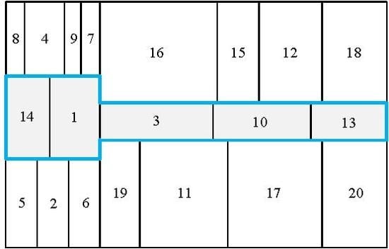
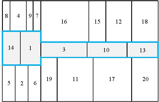
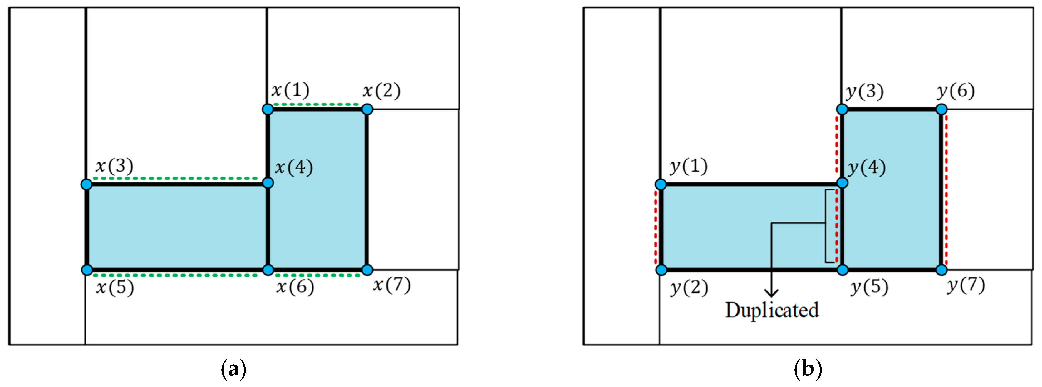
An example of this calculation is shown in Figure 2. As shown in Figure 2, the size of the loop can be calculated as the sum of the perimeter of the two departments. If we calculate separately in the and directions, it is equivalent to twice of length in the direction (Figure 2a) plus twice the length in the direction excluding the shared border of the departments (Figure 2b). The axis contains the distances of , , , and . In this case, there are no duplicated distances between the adjacent departments. The axis contains the distances of , , , and . In this case, the distance of is shared by two adjacent departments. Therefore, this duplicated distance () should be subtracted. The measurement criterion of is described in detail in Section 4.3.
4. Layout Design with MBO and Single Loop Construction
As explained in Section 3, the problems we deal with are divided into two parts: the layout design and the single loop construction. In the layout design part, we use the STS to obtain the basic layout configuration, and we determine the single loop for a given layout in the single loop construction section. MBO is used to search for a better layout, which forms the shorter single loop.
4.1. Layout Representation
An FLP needs a layout representation method to be shown its layout in a certain code. The STS is adopted as a layout representation in our study. In principle, the STS has more encoding vectors than FBS, which represent components of the STS such as the department and slicing cutting sequence. Therefore, generally, the FBS has been adopted for layout representation because of its relative simplicity [27,28]. However, by allowing both directions, the STS can offer a greater variety of layouts than the FBS, as shown in Figure 3.
Basically, the STS is composed of an internal and external node. The internal node represents the horizontal and vertical cutting direction. The external node, on the other hand, represents the sequence of departments in a layout [6].
As shown in Figure 4, the horizontal and vertical directions are symbolized as binary values. This type of STS with binary vectors was originally from [42,43]. In the authors’ papers, the STS sequence of a layout with n number of departments can be represented with leaves and nodes. In this study, an STS with three encoding sequences is adopted, as described in Figure 5. First, the department sequence (1-3-2-5-4-6) is horizontally divided into two branches (1-3 and 2-5-4-6) because the cut orientation is 2 with a cut code of 0. Next, from the given cut orientation code of 1, the sub-branch (1-3) is separated into individual departments. At this point, the inverse vertical cut occurs because the cut code is 3 rather than 1. Accordingly, the sub-branch (1-3) is separated into 3 and 1 sequentially. The other sub-branches separate in a likewise fashion. In the third step, the sub-branch (2-5-4-6) is divided into two parts vertically, (2-5) and (4-6). Sequentially, the sub-branch (2-5) is horizontally divided into individual departments (2) and (5). The other sub-branch, (4-6), is divided into (4) and (6) by a vertical cut.
Komarudin and Wong [44] first introduced this type of STS, which is composed of the department sequence, the cut orientation, and the cut code. The department sequence indicates the order of departments in a line. The cut orientation shows the location where the horizontal or vertical cut occurs. Lastly, the cut code represents the cutting direction, and this is usually composed of binary vectors. Using this structure as a basis, Kang and Chae [5] extended the cut code from 0 to 3 to represent the inverse assignment and decrease the computation time. Likewise, in this study, the cut code is represented as 0 for the horizontal direction, 1 for the vertical direction, 2 for the inverse horizontal direction and 3 for the inverse vertical direction.
4.2. Monarch Butterfly Optimization
MBO was introduced by Wang et al. [9] for the first time. Inspired by the behavior of the monarch butterfly, MBO mimics the migration patterns of this species. The monarch butterfly migrates from the northern USA and southern Canada to Mexico during the summer and autumn. In this regard, the migrating butterfly population can be divided into two groups: Land 1 and Land 2. To simplify the migration of the monarch butterfly, the butterfly individuals stay in Land 1 for four months and Land 2 for seven months. The butterfly individuals in Land 2 move to Land 1 in April. On the other hand, the butterfly individuals in Land 1 move to Land 2 in September. Accordingly, the butterflies in Land 1 () and Land 2 () compose the total butterfly population (). This can be expressed as Equations (9) and (10).
stands for the rate (%) of butterfly individuals staying in Land 1. Therefore, the subpopulation in Land 1 can be expressed as where is the nearest integer that is greater than or equal to .
After dividing the population, the new butterfly individuals in Land 1 and Land 2 can be generated by each operator in parallel (i.e., the migration operator and butterfly adjusting operator). After the operator application, the fitness values of each generated individual are evaluated. If the newly generated individual has a better fitness value than the previous one, the old parent individual is replaced with the new one via the greedy strategy, as in Equation (11) [10].
The overall process of the updating scheme can be seen in Figure 6.
As mentioned, butterflies in Land 1 and Land 2 undergo their updating process simultaneously. The migration operator, which is the operator in Land 1, is driven by a modified random number , which is a random decimal fraction multiplied by . According to the original author, can be regarded as a value of 1.2, which reflects the migration period of a 12-month a year.
| Operator 1: Migration Operator | |
| Begin | |
| for (all monarch butterfly in Subpopulation 1) | |
| if () | |
| in Subpopulation 1 | (12) |
| Else | |
| in Subpopulation 2 | (13) |
| End | |
| End | |
| End | |
In Equation (12), is an individual butterfly that has three separate representations: a department sequence, cut orientation and cut code. is the current generation. Thus, is a butterfly of the generation . Similarly, indicates an individual butterfly that is randomly selected from Subpopulation 1, and indicates the one from Subpopulation 2. The new individual from Land 1, , is randomly selected from Subpopulation 1 if is less than or equal to , as shown in Equation (12). If is greater than , a new butterfly is selected in Subpopulation 2, as shown in Equation (13). , the butterfly adjusting ratio, is set to 0.41 (5/12) in accordance with the migration period in Land 1 [9].
The butterflies in Land 2 are updated via the other updating operator, the butterfly adjusting operator.
| Operator 2: Butterfly Adjusting Operator | |
| Begin | |
| for (all monarch butterfly in Subpopulation 2) | |
| if () | |
| (14) | |
| Else | |
| in Subpopulation 2 | (15) |
| if () | |
| swap two components in the random Subpopulation | (16) |
| End | |
| End | |
| End | |
For Subpopulation 2-oriented butterflies, if the random number is lower than or equal to p, the current best butterfly individual can exist in a new generation, as in Equation (14). This ensures that the butterfly, which provides the best fitness value, continues to the next generation. On the other hand, if is greater than p, a randomly selected butterfly in Land 2 can become a new butterfly, as in Equation (15). But in the case of Equation (16), this can be modified by a butterfly adjusting rate, . If is greater than , two components in the parent butterfly are swapped randomly and this generates a new offspring. The process of swapping two departments is described in Figure 7.
By using this meta-heuristic approach with the STS, the evaluation method of an obtained layout is described in the next section.
4.3. Loop Construction Method
The single loop construction method is heuristically constructed in this study. The adjacent rule, which helps to find the adjacent relationship between departments, is modeled, and the loop sequence heuristic is established using the adjacent rules. For the candidate department and the relevant department , the adjacent rules can be defined as below.
According to Figure 8, is a coordinate from the west corner of Department on the axis. In the same way, is a coordinate from the south corner of Department on the axis. and are the horizontal and vertical length of Department on each axis, respectively. The following description is an example of the adjacent rules between Departments and on the axis. At least one adjacent rule must be satisfied. The examples of adjacent rules can be seen in Figure 9. In this process, adjacent duplication is allowed because the reverse adjacent case of the departments must be considered. As shown in Figure 10, if the departments only share a vertex, this case is not regarded as an adjacency.
- If , Departments and have an upper adjacent relationship.
- If , Departments and have a lower adjacent relationship.
- The upper two conditions are satisfied with a dual adjacent-1 relationship.
- If and , Departments and have a dual adjacent-2 relationship.
With these adjacent cases, the duplicated distance of Departments and () can be represented as follows.
| (a) Upper adjacent | |
| (b) Lower adjacent | |
| (c-1) Dual adjacent -1 | |
| (c-2) The opposite case of dual adjacent -1 | |
| (d) Dual adjacent -2 |
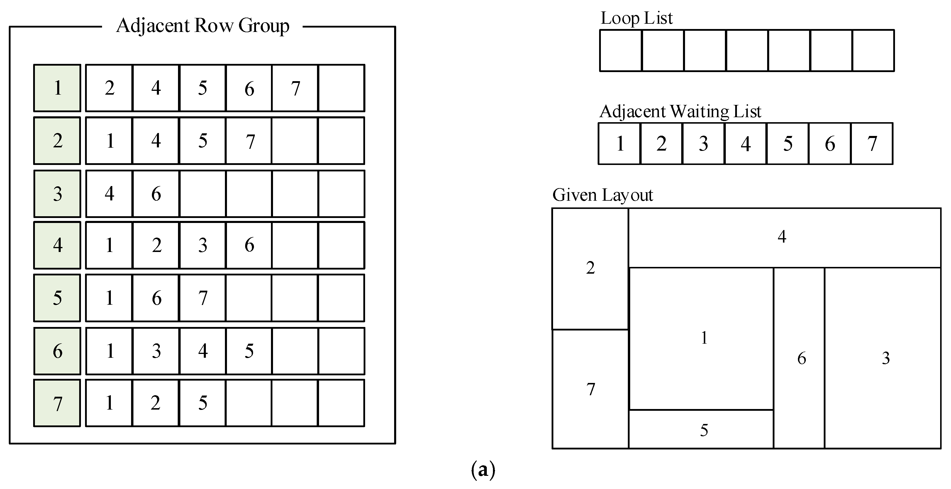
The single loop construction method follows a number of steps. In the initial stage, all departments are regarded as loop candidate departments, and each department, except the comparison target, must be compared to determine if it is adjacent to the target or not. The illustration of a single loop construction is shown in Figure 11.
- Step 0. Initialize all loop measuring sequences.
- Step 1. For all loop candidate departments, explore every adjacent department using the adjacent rules. The adjacent departments are stored in the adjacent row of each candidate target. Once the exploration is done, eliminate the duplicated departments in each adjacent row.
- Step 2. When the exploration is finished, choose one candidate department (loop department) that has the most adjacent departments and put it in the loop sequence list. Remove the adjacent row of the candidate department from the adjacent row group.
- Step 3. Remove the adjacent departments that belong to the chosen loop department from each of the adjacent rows.
- Step 4. Remove the loop department and adjacent departments that belong to the loop department from the adjacent waiting list.
- Step 5. Iterate Steps 2 to 4 until there are no remaining departments in the adjacent waiting list. When selecting the loop candidate department, it must contain the loop department as an adjacent department.
- Step 6. Measure the loop size with the departments in the loop sequence.
All lists and rows must be initialized in Step 0. Following Figure 11a, the adjacent departments are explored and stored in the adjacent row of the corresponding target department. Afterwards, in Figure 11b, the adjacent row of Department 1 with the largest number of adjacent departments is chosen to be a loop department, and this can be stored in the loop list. The adjacent departments (2, 4, 5, 6, and 7) in the adjacent row of Department 1 are now located on the loop. Therefore, they can be erased from the adjacent waiting list. However, there is still a remaining department (3) that is not located on the loop, and the next iteration must occur. Shown in Figure 11c, the adjacent row of Departments 4 and 6 have the same number of remaining departments. At this time, to minimize the loop size, the department that makes the entire size of the loop smaller can be chosen. Therefore, Department 6 can be selected. Repeating the previous iteration, Department 6 is selected as a loop department, and the adjacent department (3) can be removed from the adjacent waiting list. Because the adjacent waiting list is empty, the loop list is completed.
The single loop construction strategy proposed in this study is relatively easy to understand. Moreover, this seems to be a reasonable method to find a loop department in the layout that is constructed by using the STS because the STS can represent complicated layouts.
5. Computational Results
5.1. Experiment Information
The computational experiments with a set of well-known instances were tested to evaluate the performance of the proposed algorithms. The program was coded in JAVA, and the experiment was conducted on a computer with an Intel Core i5 CPU processor (3.5 GHz) and 8 GB of memory. The parameter setting for the experiment can be seen in Table 2.
, the total number of butterfly individuals, is set as equal to the number of departments of each instance. The size of correspondingly increases when the amount of instances increases to secure the diversification of a solution set. The remainders are set following the original parameter setting of [9]. Many studies using MBO [10,11,12,14,35] have adopted this same parameter setting because the original setting was based on the bio-inspired migration rate of the monarch butterfly.
Information regarding well-known instances is introduced in Table 3. From FO7 to AB20, the sum of every department’s size is the same as the given floor space. For the vC10s problem, the minimum length of the department is given as 5 instead of the aspect ratio. KC15 and KC25 are introduced in this study for the first time to estimate the performance of the algorithm under the problem diversity. The area information of KC15 and KC25 can be confirmed in Table A1 and Table A2. The compactness of SC30 and SC35 are less than 1.0. Simply speaking, the sum of the department’s area sizes is less than the given floor size. Therefore, the empty spaces are regarded as dummy departments in this study. It is unnecessary for the dummy departments to be located along the loop, and their aspect ratio is assumed to be free.
5.2. Experiment Results
Several well-known instances from 7 to 62 departments are tested to evaluate the performance of the algorithm. The best OFV, the average OFV, and the corresponding computation time can be seen in Table 4. Since the STS can show the cutting style that can be obtained from both FBS and STS, as shown in Figure 12 and Figure 13, the obtained layouts of FO7, FO8, FO9, and vC10a tend to have a bay-cutting layout form, which can also be derived by the FBS. On the other hand, the rest of the layouts are composed of both vertical and horizontal cuts that can be easily seen in the STS representation, as shown in Figure 13, Figure 14, Figure 15 and Figure 16. It can be said that that as the number of departments increases, the layout tends to have an STS-like look.
To the best of our knowledge, there is no previous literature that solves the UAFLP with the objective of determining the shortest single loop distance. Therefore, a direct comparison to the objective function used in other methods would not be appropriate. However, a comparison of computation times for similar instances would offer a clue in terms of the performance of the proposed MBO. Table 5 compares the present results with those provided by Asef-vaziri et al. [28]. Their approach is similar in that the pre-defined layout representation is used with a meta-heuristic to determine the layout design based on a single loop. The objective function and the values in [28] are different, as mentioned. The objective of [28] includes the loaded and empty flow between pairs of I/O points, while this study finds the shortest single loop material handling path. There are several factors that affect computation time. The computer system could be one of them. The results in [28] are generated from an 8GB RAM computer with a core-i7 CPU, while this study uses an 8GB RAM computer with a core-i5 CPU. Data structure also affects the computation time. AB20 is the only instance that uses both methods, and the proposed method provides a slightly faster CPU time. We are able to confirm that the proposed heuristic and MBO in this study can solve the problem in a relatively reasonable computation time, as shown in Table 4.
The layout configurations of SC30 and SC35 are shown in Figure 15. The area compactness of SC30 and SC35 is less than 1. That means the floor space is greater than the total department area. Thus, the dummy departments are included to solve the problem in the given layout structure. The departments, for which the numbers are greater than the given problem size in Figure 15, are the dummy department. For instance, department 38 in Figure 15b is one of the dummy departments, and thus, the single loop does not need to proceed through to any segment of the department. Figure 16 shows the layout configuration of DU62, and this problem does not include the dummy department.
6. Conclusions
Facility layout problems (FLPs) are placement problems that consider changes in the width and height of non-overlapping departments in a certain space. Several distance measurements, including the rectilinear distance or Euclidean distance, have been suggested to evaluate the obtained layout. However, these distance measurements are not appropriate for certain material handling systems such as circulating AVGs or power and free systems. Therefore, to determine a layout that considers the usage of circulating path-based equipment, we proposed a single loop construction method with a meta-heuristic, MBO. The MBO mimics the monarch butterfly’s migration patterns. Its performance has been verified in various optimization problems. The MBO is relatively easy to apply and modify compared to other evolutionary algorithms because it has very simple operators and parameter sets.
The objective function of this study is the single loop size minimization for the circulating material handling equipment path. To evaluate the objective function values (OFVs), a single loop construction method that finds the single loop while minimizing the OFVs was introduced.
To evaluate the algorithm performance, several well-known instances were tested. MBO successfully found the single loop in a reasonable amount of time. The proposed algorithm tends to generate favorable solutions. Further studies can search for better layout placements considering better loop construction heuristics with reduced computation times. Additionally, improving MBO with other powerful methods could yield potential developments. As mentioned, to generate better solutions with MBO, some researchers took specific operators from other meta-heuristic algorithms. It might be a meaningful challenge to find different operators which fit with MBO.
Author Contributions
Conceptualization, M.K. and J.C.; methodology, M.K.; software, M.K.; validation, M.K. and J.C.; formal analysis, M.K.; investigation, M.K.; resources, J.C.; data curation, M.K.; writing—original draft preparation, M.K.; writing—review and editing, J.C.; visualization, M.K.; supervision, J.C.; project administration, J.C.; funding acquisition, J.C.
Funding
This work was supported by a 2017 Korea Aerospace University faculty research grant.
Conflicts of Interest
The authors declare no conflict of interest.
Appendix A
The instances used in this study is basically brought from other papers. However, two instances were created in this study for department size of 15 and 25. The specific area information of the new instances as follows.

Table A1.
The department area of KC15.
| Department number | 1 | 2 | 3 | 4 | 5 | 6 | 7 | 8 | 9 | 10 | 11 | 12 | 13 | 14 | 15 |
| Area | 0.5 | 0.4 | 0.6 | 0.18 | 0.45 | 0.45 | 0.45 | 0.45 | 0.21 | 0.1 | 0.74 | 0.42 | 0.25 | 0.5 | 0.3 |
Table A2.
The department area of KC25.
| Department number | 1 | 2 | 3 | 4 | 5 | 6 | 7 | 8 | 9 | 10 | 11 | 12 | 13 | 14 | 15 |
| Area | 0.33 | 0.5 | 0.4 | 0.38 | 0.45 | 0.49 | 0.45 | 0.24 | 0.14 | 0.3 | 0.3 | 0.42 | 0.25 | 0.5 | 0.3 |
| Department number | 16 | 17 | 18 | 19 | 20 | 21 | 22 | 23 | 24 | 25 | |||||
| Area | 0.45 | 0.51 | 0.44 | 0.34 | 0.3 | 0.43 | 0.24 | 0.3 | 0.3 | 0.24 |
References
- Tompkins, J.A.; White, J.A.; Bozer, Y.A.; Tanchoco, J.M.A. Facilities Planning, 4th ed.; John Wiley & Sons: Hoboken, NJ, USA, 2010. [Google Scholar]
- Kusiak, A.; Heragu, S.S. The facility layout problem. Eur. J. Oper. Res. 1987, 29, 229–251. [Google Scholar] [CrossRef]
- Ingole, S.; Singh, D. Unequal-area, fixed-shape facility layout problems using the firefly algorithm. Eng. Optim. 2017, 49, 1097–1115. [Google Scholar] [CrossRef]
- Tate, D.M.; Smith, A.E. Unequal-area facility layout by genetic search. IIE Trans. 1995, 27, 465–472. [Google Scholar] [CrossRef]
- Kang, S.; Chae, J. Harmony search for the layout design of an unequal area facility. Expert Syst. Appl. 2017, 79, 269–281. [Google Scholar] [CrossRef]
- Drira, A.; Pierreval, H.; Hajri-Gabouj, S. Facility layout problems: A survey. Annu. Rev. Control 2007, 31, 255–267. [Google Scholar] [CrossRef]
- Shouman, M.A.; Nawara, G.M.; Reyad, A.H.; El-darandaly, K. Facility layout problem (FLP) and intelligent techniques: a survey. In Proceedings of the 7th International Conference on Production Engineeering, Design and Control(PEDAC), Alexandria, Egypt, 13–15 February 2001; pp. 409–422. [Google Scholar]
- Meller, R.D.; Gau, K.Y. The facility layout problem: Recent and emerging trends and perspectives. J. Manuf. Syst. 1996, 15, 351–366. [Google Scholar] [CrossRef]
- Wang, G.-G.; Deb, S.; Cui, Z. Monarch butterfly optimization. Neural Comput. Appl. 2015, 1–20. [Google Scholar] [CrossRef]
- Chen, S.; Chen, R.; Gao, J. A Monarch Butterfly Optimization for the Dynamic Vehicle Routing Problem. Algorithms 2017, 10, 107. [Google Scholar] [CrossRef]
- Ghetas, M.; Yong, C.H.; Sumari, P. Harmony-based monarch butterfly optimization algorithm. In 2015 IEEE International Conference on Control System, Computing and Engineering (ICCSCE); IEEE: George Town, Malaysia, 2015; pp. 156–161. [Google Scholar]
- Wang, G.-G.; Hao, G.-S.; Cheng, S.; Qin, Q. A Discrete Monarch Butterfly Optimization for Chinese TSP Problem. In International Conference in Swarm Intelligence; Springer: Cham, Switzerland, 2016; Volume 9712, pp. 165–173. [Google Scholar]
- Wang, G.-G.; Deb, S.; Zhao, X.; Cui, Z. A new monarch butterfly optimization with an improved crossover operator. Oper. Res. 2018, 18, 731–755. [Google Scholar] [CrossRef]
- Wang, G.-G.; Zhao, X.; Deb, S. A Novel Monarch Butterfly Optimization with Greedy Strategy and Self-Adaptive. In 2015 Second International Conference on Soft Computing and Machine Intelligence (ISCMI); IEEE: Hong Kong, China, 2015; pp. 45–50. [Google Scholar]
- Chittratanawat, S.; Noble, J.S. An integrated approach for facility layout, P/D location and material handling system design. Int. J. Prod. Res. 1999, 37, 683–706. [Google Scholar] [CrossRef]
- Kochhar, J.S.; Foster, B.T.; Heragu, S.S. HOPE: A genetic algorithm for the unequal area facility layout problem. Comput. Oper. Res. 1998, 25, 583–594. [Google Scholar] [CrossRef]
- Scholz, D.; Petrick, A.; Domschke, W. STaTS: A Slicing Tree and Tabu Search based heuristic for the unequal area facility layout problem. Eur. J. Oper. Res. 2009, 197, 166–178. [Google Scholar] [CrossRef]
- Bukchin, Y.; Tzur, M. A new MILP approach for the facility process-layout design problem with rectangular and L/T shape departments. Int. J. Prod. Res. 2014, 52, 7339–7359. [Google Scholar] [CrossRef]
- Gonçalves, J.F.; Resende, M.G.C. A biased random-key genetic algorithm for the unequal area facility layout problem. Eur. J. Oper. Res. 2015, 246, 86–107. [Google Scholar] [CrossRef]
- Asef-Vaziri, A.; Kazemi, M. Covering and connectivity constraints in loop-based formulation of material flow network design in facility layout. Eur. J. Oper. Res. 2018, 264, 1033–1044. [Google Scholar] [CrossRef]
- Sinriech, D.; Tanchoco, J.M.A. Solution methods for the mathematical models of single-loop AGV systems. Int. J. Prod. Res. 1993, 31, 705–725. [Google Scholar] [CrossRef]
- Tanchoco, J.M.A.; Sinriech, D. OSL—optimal single-loop guide paths for AGVS. Int. J. Prod. Res. 1992, 30, 665–681. [Google Scholar] [CrossRef]
- Asef-Vaziri, A.; Laporte, G.; Sriskandarajah, C. The block layout shortest loop design problem. IIE Trans. 2000, 32, 727–734. [Google Scholar] [CrossRef]
- Ahmadi-Javid, A.; Ramshe, N. On the block layout shortest loop design problem. IIE Trans. 2013, 45, 494–501. [Google Scholar] [CrossRef]
- Yang, T.; Peters, B.A.; Tu, M. Layout design for flexible manufacturing systems considering single-loop directional flow patterns. Eur. J. Oper. Res. 2005, 164, 440–455. [Google Scholar] [CrossRef]
- Hojabri, H.; Hojabri, A.; Jaafari, A.A.; Farahani, L.N. A Loop Material Flow System Design. Eng. Comput. Sci. 2010, 3, 1544–1545. [Google Scholar]
- Jahandideh, H.; Asef-Vaziri, A.; Modarres, M. Genetic Algorithm for Designing a Convenient Facility Layout for a Circular Flow Path. Available online: https://arxiv.org/vc/arxiv/papers/1211/1211.2361v1.pdf (accessed on 6 December 2018).
- Asef-Vaziri, A.; Jahandideh, H.; Modarres, M. Loop-based facility layout design under flexible bay structures. Int. J. Prod. Econ. 2017, 193, 713–725. [Google Scholar] [CrossRef]
- Chae, J.; Peters, B.A. A simulated annealing algorithm based on a closed loop layout for facility layout design in flexible manufacturing systems. Int. J. Prod. Res. 2006, 44, 2561–2572. [Google Scholar] [CrossRef]
- Niroomand, S.; Hadi-Vencheh, A.; Şahin, R.; Vizvári, B. Modified migrating birds optimization algorithm for closed loop layout with exact distances in flexible manufacturing systems. Expert Syst. Appl. 2015, 42, 6586–6597. [Google Scholar] [CrossRef]
- Kang, S.; Kim, M.; Chae, J. A closed loop based facility layout design using a cuckoo search algorithm. Expert Syst. Appl. 2018, 93, 322–335. [Google Scholar] [CrossRef]
- Asef-Vaziri, A.; Laporte, G. Loop based facility planning and material handling. Eur. J. Oper. Res. 2005, 164, 1–11. [Google Scholar] [CrossRef]
- Kulturel-Konak, S.; Konak, A. Linear Programming Based Genetic Algorithm for the Unequal Area Facility Layout Problem. Int. J. Prod. Res. 2013, 51, 4302–4324. [Google Scholar] [CrossRef]
- Azadivar, F.; Wang, J. Facility layout optimization using simulation and genetic algorithms. Int. J. Prod. Res. 2000, 38, 4369–4383. [Google Scholar] [CrossRef]
- Ghanem, W.A.H.M.; Jantan, A. Hybridizing artificial bee colony with monarch butterfly optimization for numerical optimization problems. Neural Comput. Appl. 2018, 30, 163–181. [Google Scholar] [CrossRef]
- Montreuil, B. A Modelling Framework for Integrating Layout Design and flow Network Design. In Material Handling ’90; Springer: Berlin, Heidelberg, 1991; Volume 2, pp. 95–115. ISBN 978-3-642-84356-3. [Google Scholar]
- Meller, R.D.; Narayanan, V.; Vance, P.H. Optimal facility layout design. Oper. Res. Lett. 1998, 23, 117–127. [Google Scholar] [CrossRef]
- Sherali, H.D.; Fraticelli, B.M.P.; Meller, R.D. Enhanced Model Formulations for Optimal Facility Layout. Oper. Res. 2003, 51, 629–644. [Google Scholar] [CrossRef]
- Castillo, I.; Westerlund, T. An ε-accurate model for optimal unequal-area block layout design. Comput. Oper. Res. 2005, 32, 429–447. [Google Scholar] [CrossRef]
- Farahani, R.Z.; Laporte, G.; Sharifyazdi, M. A practical exact algorithm for the shortest loop design problem in a block layout. Int. J. Prod. Res. 2005, 43, 1879–1887. [Google Scholar] [CrossRef]
- Asef-Vaziri, A.; Ortiz, R.A. The value of the shortest loop covering all work centers in a manufacturing facility layout. Int. J. Prod. Res. 2008, 46, 703–722. [Google Scholar] [CrossRef]
- Tam, K.Y. Genetic algorithms, function optimization, and facility layout design. Eur. J. Oper. Res. 1992, 63, 322–346. [Google Scholar] [CrossRef]
- Tam, K.Y. A simulated annealing algorithm for allocating space to manufacturing cells. Int. J. Prod. Res. 1992, 30, 63–87. [Google Scholar] [CrossRef]
- Komarudin, K.; Wong, K.Y. Applying Ant System for solving Unequal Area Facility Layout Problems. Eur. J. Oper. Res. 2010, 202, 730–746. [Google Scholar] [CrossRef]
- van Camp, D.J.; Carter, M.W.; Vannelli, A. A nonlinear optimization approach for solving facility layout problems. Eur. J. Oper. Res. 1992, 57, 174–189. [Google Scholar] [CrossRef]
- Armour, G.C.; Buffa, E.S. A Heuristic Algorithm and Simulation Approach to Relative Location of Facilities. Manage. Sci. 1963, 9, 294–309. [Google Scholar] [CrossRef]
- Liu, Q.; Meller, R.D. A sequence-pair representation and MIP-model- based heuristic for the facility layout problem with rectangular departments. IIE Trans. 2007, 39, 377–394. [Google Scholar] [CrossRef]
- Dunker, T.; Radons, G.; Westkämper, E. A coevolutionary algorithm for a facility layout problem. Int. J. Prod. Res. 2003, 41, 3479–3500. [Google Scholar] [CrossRef]
Figure 1.
Examples of distance measurement. (a) Rectilinear distance; (b) Contour distance; (c) Single loop distance; (d) Euclidean distance.
Figure 1.
Examples of distance measurement. (a) Rectilinear distance; (b) Contour distance; (c) Single loop distance; (d) Euclidean distance.

Figure 2.
Loop distance measurements. (a) On the axis; (b) On the axis.

Figure 3.
Layout representation. (a) Flexible bay structure; (b) Slicing tree structure.

Figure 4.
An example of the slicing tree structure. (a) Layout representation; (b) Tree structure.

Figure 5.
Slicing tree encoding scheme.

Figure 6.
Updating process of MBO. (a) Migration operator; (b) Butterfly adjusting operator.

Figure 7.
Swapping process.

Figure 8.
The example of coordinates.

Figure 9.
Examples of adjacent cases. (a) Upper adjacent; (b) Lower adjacent; (c) Dual adjacent-1; (d) Dual adjacent-2.
Figure 9.
Examples of adjacent cases. (a) Upper adjacent; (b) Lower adjacent; (c) Dual adjacent-1; (d) Dual adjacent-2.

Figure 10.
A case with non-contiguous departments.

Figure 11.
Single loop construction steps. (a) Step 1; (b) Steps 2–4 with Iteration 1; (c) Steps 2–4 with Iteration 2.
Figure 11.
Single loop construction steps. (a) Step 1; (b) Steps 2–4 with Iteration 1; (c) Steps 2–4 with Iteration 2.


Figure 12.
Layout configurations. (a) FO7; (b) FO8; (c) FO9.

Figure 13.
Layout configurations. (a) vC10s; (b) vC10a; (c) KC15.

Figure 14.
Layout configurations. (a) AB20; (b) KC25.

Figure 15.
Layout configurations. (a) SC30; (b) SC35.

Figure 16.
Layout configuration for DU62.

Table 1.
Parameters and variables.
| Parameters and Variables | |
|---|---|
| The number of departments | |
| The or size of the floor space, where | |
| The or size of the department | |
| The valid lower bound and upper bound of | |
| The centroid coordinate of department in a direction of | |
| The south-west coordinate of department in a direction of | |
| The size of the single loop. | |
| 1, when the department is on the left of the . 0, otherwise | |
| 1, when the department is lower than that of the . 0, otherwise | |
Table 2.
Parameters used in MBO.
| Name | Rate |
|---|---|
| No. of departments | |
| 5/12 | |
| 5/12 | |
| 1.2 |
Table 3.
The instance information.
| Name | Number of Departments | Floor Space | Shape Constraint | Reference |
|---|---|---|---|---|
| FO7 | 7 | 8.5413.00 | ar = 5 | Meller et al. [37] |
| FO8 | 8 | 11.3113.00 | ar = 5 | Meller et al. [37] |
| FO9 | 9 | 12.0013.00 | ar = 5 | Meller et al. [37] |
| vC10s | 10 | 25.00 | = 5 | van Camp et al. [45] |
| vC10a | 10 | 25.0051.00 | ar = 5 | van Camp et al. [45] |
| KC15 | 15 | 2.003.00 | ar = 3 | This study |
| AB20 | 20 | 2.003.00 | ar = 4 | Armour and Buffa [46] |
| KC25 | 25 | 3.003.00 | ar = 4 | This study |
| SC30 | 30 | 15.0012.00 | ar = 5 | Liu and Meller [47] |
| SC35 | 35 | 16.0015.00 | ar = 4 | Liu and Meller [47] |
| DU62 | 62 | 117.124117.124 | ar = 4 | Dunker et al. [48] |
Table 4.
The experiment results.
| Name | Best OFV | Best’s CPU Time | Average OFV | Average CPU Time |
|---|---|---|---|---|
| FO7 | 12.10 | 10.56 | 13.10 | 11.03 |
| FO8 | 12.01 | 9.10 | 16.80 | 13.82 |
| FO9 | 12.82 | 12.85 | 15.14 | 14.37 |
| vC10s | 72.84 | 30.13 | 80.24 | 41.62 |
| vC10a | 43.81 | 35.03 | 48.16 | 38.74 |
| KC15 | 4.89 | 40.45 | 6.12 | 41.82 |
| AB20 | 6.00 | 91.42 | 8.97 | 93.52 |
| KC25 | 9.18 | 103.59 | 13.05 | 118.40 |
| SC30 | 36.78 | 412.38 | 59.13 | 406.67 |
| SC35 | 54.50 | 778.52 | 86.24 | 711.49 |
| DU62 | 509.41 | 1151.37 | 722.63 | 1104.65 |
Table 5.
The computation time comparison.
| This Study | Asef-vaziri et al. [28] | ||||
|---|---|---|---|---|---|
| Problem | Average OFV | Average CPU time | Problem | Average OFV | CPU time |
| FO7 | 13.10 | 11.03 | |||
| FO8 | 16.80 | 13.82 | |||
| FO9 | 15.14 | 14.37 | |||
| vC10s | 80.24 | 41.62 | vC10 | 2.32 | 24.00 |
| vC10a | 48.16 | 38.74 | |||
| KC15 | 6.12 | 41.82 | ML15 | 2.22 | 60.00 |
| AB20 | 8.97 | 93.52 | AB20 | 1.25 | 101.00 |
| KC25 | 13.05 | 118.40 | ML25 | 2.03 | 181.00 |
| SC30 | 59.13 | 406.67 | TA30 | 1.57 | 471.00 |
| SC35 | 86.24 | 711.49 | KG37 | 2.06 | 507.00 |
| DU62 | 722.63 | 1104.65 | DE62 | 1.38 | 1487.00 |
© 2019 by the authors. Licensee MDPI, Basel, Switzerland. This article is an open access article distributed under the terms and conditions of the Creative Commons Attribution (CC BY) license (http://creativecommons.org/licenses/by/4.0/).
Share and Cite
MDPI and ACS Style
Kim, M.; Chae, J. Monarch Butterfly Optimization for Facility Layout Design Based on a Single Loop Material Handling Path. Mathematics 2019, 7, 154. https://doi.org/10.3390/math7020154
AMA Style
Kim M, Chae J. Monarch Butterfly Optimization for Facility Layout Design Based on a Single Loop Material Handling Path. Mathematics. 2019; 7(2):154. https://doi.org/10.3390/math7020154
Chicago/Turabian StyleKim, Minhee, and Junjae Chae. 2019. "Monarch Butterfly Optimization for Facility Layout Design Based on a Single Loop Material Handling Path" Mathematics 7, no. 2: 154. https://doi.org/10.3390/math7020154
Note that from the first issue of 2016, this journal uses article numbers instead of page numbers. See further details here.