Enhancing Elephant Herding Optimization with Novel Individual Updating Strategies for Large-Scale Optimization Problems

Changchun Institute of Optics, Fine Mechanics and Physics, Chinese Academy of Sciences, Changchun 130033, China
*
Author to whom correspondence should be addressed.
Mathematics 2019, 7(5), 395; https://doi.org/10.3390/math7050395
Submission received: 16 February 2019
/
Revised: 26 April 2019
/
Accepted: 27 April 2019
/
Published: 30 April 2019
(This article belongs to the Special Issue Evolutionary Computation)
Abstract
:Inspired by the behavior of elephants in nature, elephant herd optimization (EHO) was proposed recently for global optimization. Like most other metaheuristic algorithms, EHO does not use the previous individuals in the later updating process. If the useful information in the previous individuals were fully exploited and used in the later optimization process, the quality of solutions may be improved significantly. In this paper, we propose several new updating strategies for EHO, in which one, two, or three individuals are selected from the previous iterations, and their useful information is incorporated into the updating process. Accordingly, the final individual at this iteration is generated according to the elephant generated by the basic EHO, and the selected previous elephants through a weighted sum. The weights are determined by a random number and the fitness of the elephant individuals at the previous iteration. We incorporated each of the six individual updating strategies individually into the basic EHO, creating six improved variants of EHO. We benchmarked these proposed methods using sixteen test functions. Our experimental results demonstrated that the proposed improved methods significantly outperformed the basic EHO.
1. Introduction
Inspired by nature, a large variety of metaheuristic algorithms [1] have been proposed that provide optimal or near-optimal solutions to various complex large-scale problems that are difficult to solve using traditional techniques. Some of the many successful metaheuristic approaches include particle swarm optimization (PSO) [2,3], cooperative coevolution [4,5,6], seagull optimization algorithm [7], GRASP [8], clustering algorithm [9], and differential evolution (DE) [10,11], among others.
In 2015, Wang et al. [12,13] proposed a new metaheuristic algorithm called elephant herd optimization (EHO), for finding the optimal or near-optimal function values. Although EHO exhibits a good performance on benchmark evaluations [12,13], like most other metaheuristic methods, it does not utilize the best information from the previous elephant individuals to guide current and future searches. This gap will be addressed, because previous individuals can provide a variety of useful information. If such information could be fully exploited and applied in the later updating process, the performance of EHO may be improved significantly, without adding unnecessary operations and fitness evaluations.
In the research presented in this paper, we extended and improved the performance of the original EHO (which we call “the basic EHO”) by fully investigating the information in the previous elephant individuals. Then, we designed six updating strategies to update the individuals. For each of the six individual updating strategies, first, we selected a certain number of elephants from the previous iterations. This selection could be made in either a fixed or random way, with one, two, or three individuals selected from previous iterations. Next, we used the information from these selected previous individual elephants to update the individuals. In this way, the information from the previous individuals could be reused fully. The final elephant individual at this iteration was generated according to the elephant individual generated by the basic EHO at the current iteration, along with the selected previous elephants using a weighted sum. While there are many ways to determine the weights, in our current work, they were determined by random numbers. Last, by combining the six individual updating strategies with EHO, we developed the improved variants of EHO. To verify our work, we benchmarked these variants using sixteen cases involving large-scale complex functions. Our experimental results showed that the proposed variants of EHO significantly outperformed the originally described EHO.
The organization of the remainder of this paper is as follows. Section 2 reviews the main steps of the basic EHO. In Section 3, we describe the proposed method for incorporating useful information from previous elephants into the EHO. Section 4 provides details of our various experiments on sixteen large-scale functions. Lastly, Section 5 offers our conclusion and suggestions for future work.
2. Related Work
As EHO [12,13] is a newly-proposed swarm intelligence-based algorithm, in this section, some of the most representative work regarding swarm intelligence, including EHO, are summarized and reviewed.
Meena et al. [14] proposed an improved EHO algorithm, which is used to solve the multi-objective distributed energy resources (DER) accommodation problem of distribution systems by combining a technique for order of preference by similarity to ideal solution (TOPSIS). The proposed technique is productively implemented on three small- to large-scale benchmark test distribution systems of 33-bus, 118-bus, and 880-bus.
When the spectral resolution of the satellite imagery is increased, the higher within-class variability reduces the statistical separability between the LU/LC classes in spectral space and tends to continue diminishing the classification accuracy of the traditional classifiers. These are mostly per pixel and parametric in nature. Jayanth et al. [15] used EHO to solve the problems. The experimental results revealed that EHO shows an improvement of 10.7% on Arsikere Taluk and 6.63% on the NITK campus over the support vector machine.
Rashwan et al. [16] carried out a series of experiments on a standard test bench, as well as engineering problems and real-world problems, in order to understand the impact of the control parameters. On top of that, the main aim of this paper is to propose different approaches to enhance the performance of EHO. Case studies ranging from the recent test bench problems of Congress on Evolutionary Computation (CEC) 2016, to the popular engineering problems of the gear train, welded beam, three-bar truss design problem, continuous stirred tank reactor, and fed-batch fermentor, are used to validate and test the performances of the proposed EHOs against existing techniques.
Correia et al. [17] firstly used a metaheuristic algorithm, namely EHO, to address the energy-based source localization problem in wireless sensor networks. Through extensive simulations, the key parameters of the EHO algorithm are optimized, such that they match the energy decay model between two sensor nodes. The simulation results show that the new approach significantly outperforms the existing solutions in noisy environments, encouraging further improvement and testing of metaheuristic methods.
Jafari et al. [18] proposed a new hybrid algorithm that was based on EHO and cultural algorithm (CA), known as the elephant herding optimization cultural (EHOC) algorithm. In this process, the belief space defined by the cultural algorithm was used to improve the standard EHO. In EHOC, based on the belief space, the separating operator is defined, which can create new local optimums in the search space, so as to improve the algorithm search ability and to create an algorithm with an optimal exploration–exploitation balance. The CA, EHO, and EHOC algorithms are applied to eight mathematical optimization problems and four truss weight minimization problems, and to assess the performance of the proposed algorithm, the results are compared. The results clearly indicate that EHOC can accelerate the convergence rate effectively and can develop better solutions compared with CA and EHO.
Hassanien et al. [19] combined support vector regression (SVR) with EHO in order to predict the values of the three emotional scales as continuous variables. Multiple experiments are applied to evaluate the prediction performance. EHO was applied in two stages of the optimization. Firstly, to fine-tune the regression parameters of the SVR. Secondly, to select the most relevant features extracted from all 40 EEG channels, and to eliminate the ineffective and redundant features. To verify the proposed approach, the results proved EHO-SVR’s ability to gain a relatively enhanced performance, measured by a regression accuracy of 98.64%.
Besides EHO, many other swarm intelligence-based algorithms have been proposed, and some of the most representative ones are summarized and reviewed as follows.
Monarch butterfly optimization (MBO) [20] is proposed for global optimization problems, inspired by the migration behavior of monarch butterflies. Yi et al. [21] proposed a novel quantum inspired MBO methodology, called QMBO, by incorporating quantum computation into MBO, which is further used to solve uninhabited combat air vehicles (UCAV) path planning navigation problem [22,23]. In addition, Feng et al. proposed various variants of MBO algorithms to solve the knapsack problem [24,25,26,27,28]. In addition, Wang et al. also improved on the performance of the MBO algorithm from various aspects [29,30,31,32]; a variant of the MBO method in combination with two optimization strategies, namely GCMBO, was also put forward.
Inspired by the phototaxis and Lévy flights of the moths, Wang developed a new kind of metaheuristic algorithm, called the moth search (MS) algorithm [33]. Feng et al. [34] divided twelve transfer functions into three families, and combined them with MS, and then twelve discrete versions of MS algorithms are proposed for solving the set-union knapsack problem (SUKP). Based on the improvement of the moth search algorithm (MSA) using differential evolution (DE), Elaziz et al. [35] proposed a new method for the cloud task scheduling problem. In addition, Feng and Wang [36] verified the influence of the Lévy flights operator and fly straightly operator in MS. Nine types of new mutation operators based on the global harmony search have been specially devised to replace the Lévy flights operator.
Inspired by the herding behavior of krill, Gandomi and Alavi proposed a krill herd (KH) [37]. After that, Wang et al. improved the KH algorithms through different optimization strategies [38,39,40,41,42,43,44,45,46]. More literature regarding the KH algorithm can be found in the literature [47].
The artificial bee colony (ABC) algorithm [48] is a swarm-based meta-heuristic algorithm that was introduced by Karaboga in 2005 for optimizing numerical problems. Wang and Yi [49] presented a robust optimization algorithm, namely KHABC, based on hybridization of KH and ABC methods and the information exchange concept. In addition, Liu et al. [50] presented an ABC algorithm based on the dynamic penalty function and Lévy flight (DPLABC) for constrained optimization problems.
Also, many other researchers have proposed other state-of-the-art metaheuristic algorithms, such as particle swarm optimization (PSO) [51,52,53,54,55,56], cuckoo search (CS) [57,58,59,60,61], probability-based incremental learning (PBIL) [62], differential evolution (DE) [63,64,65,66], evolutionary strategy (ES) [67,68], monarch butterfly optimization (MBO) [20], firefly algorithm (FA) [69,70,71,72], earthworm optimization algorithm (EWA) [73], genetic algorithms (GAs) [74,75,76], ant colony optimization (ACO) [77,78,79], krill herd (KH) [37,80,81], invasive weed optimization [82,83,84], stud GA (SGA) [85], biogeography-based optimization (BBO) [86,87], harmony search (HS) [88,89,90], and bat algorithm (BA) [91,92], among others
Besides benchmark evaluations [93,94], these proposed state-of-the-art metaheuristic algorithms are also used to solve various practical engineering problems, like test-sheet composition [95], scheduling [96,97], clustering [98,99,100], cyber-physical social systems [101], economic load dispatch [102,103], fault diagnosis [104], flowshop [105], big data optimization [106,107], gesture segmentation [108], target recognition [109,110], prediction of pupylation sites [111], system identification [112], shape design [113], multi-objective optimization [114], and many-objective optimization [115,116,117].
3. Elephant Herd Optimization
The basic EHO can be described using the following simplified rules [12]:
- (1)
- Elephants belonging to different clans live together led by a matriarch. Each clan has a fixed number of elephants. For the purposes of modelling, we assume that each clan consists of an equal, unchanging number of elephants.
- (2)
- The positions of the elephants in a clan are updated based on their relationship to the matriarch. EHO models this behavior through an updating operator.
- (3)
- Mature male elephants leave their family groups to live alone. We assume that during each generation, a fixed number of male elephants leave their clans. Accordingly, EHO models the updating process using a separating operator.
- (4)
- Generally, the matriarch in each clan is the eldest female elephant. For the purposes of modelling and solving the optimization problems, the matriarch is considered the fittest elephant individual in the clan.
As this paper is focused on improving the EHO updating process, in the following subsection, we provide further details of the EHO updating operator as it was originally presented. For details regarding the EHO separating operator, see the literature [12].
3.1. Clan Updating Operator
The following updating strategy of the basic EHO was described by the authors of [12], as follows. Assume that an elephant clan is denoted as ci. The next position of any elephant, j, in the clan is updated using (1), as follows:
where xnew,ci,j is the updated position, and xci,j is the prior position of elephant j in clan ci. xbest,ci denotes the matriarch of clan ci; she is the fittest elephant individual in the clan. The scale factor determines the influence of the matriarch of ci on xci,j. , which is a type of stochastic distribution, can provide a significant improvement for the diversity of the population in the later search phase. For the present work, a uniform distribution was used.
It should be noted that xci,j = xbest,ci,, which means that the matriarch (fittest elephant) in the clan cannot be updated by (1). To avoid this situation, we can update the fittest elephant using the following equation:
where the influence of xcenter,ci on xnew,ci, is regulated by .
In Equation (2), the information from all of the individuals in clan ci is used to create the new individual xnew,ci,j. The centre of clan ci, xcenter,ci, can be calculated for the d-th dimension through D calculations, where D is the total dimension, as follows:
Here, 1 ≤ d ≤ D represents the d-th dimension, nci is the number of individuals in ci, and xci,j,d is the d-th dimension of the individual xci,j.
Algorithm 1 provides the pseudocode for the updating operator.
| Algorithm 1: Clan updating operator [12] |
| Begin |
| for ci = 1 to nClan (for all clans in elephant population) do |
| for j = 1 to nci (for all elephant individuals in clan ci) do |
| Update xci,j and generate xnew,ci,j according to (1). |
| if xci,j = xbest,ci then |
| Update xci,j and generate xnew,ci,j according to (2). |
| end if |
| end for j |
| end for ci |
| End. |
3.2. Separating Operator
In groups of elephants, male elephants leave their family group and live alone upon reaching puberty. This process of separation can be modeled into a separating operator when solving optimization problems. In order to further improve the search ability of the EHO method, let us assume that the individual elephants with the worst fitness will implement the separating operator for each generation, as shown in (4).
where xmax and xmin are the upper and lower bound, respectively, of the position of the individual elephant. xworst,ci is the worst individual elephant in clan ci. is a kind of stochastic distribution, and the uniform distribution in the range [0, 1] is used in our current work.
Accordingly, the separating operator can be formed, as shown in Algorithm 2.
| Algorithm 2: Separating operator |
| Begin |
| for ci =1 to nClan (all of the clans in the elephant population) do |
| Replace the worst elephant individual in clan ci using (4). |
| end for ci |
| End. |
3.3. Schematic Presentation of the Basic EHO Algorithm
For EHO, like the other metaheuristic algorithms, a kind of elitism strategy is used with the aim of protecting the best elephant individuals from being ruined by the clan updating and separating operators. In the beginning, the best elephant individuals are saved, and the worst ones are replaced by the saved best elephant individuals at the end of the search process. This elitism ensures that the later elephant population is not always worse than the former one. The schematic description can be summarized as shown in Algorithm 3.
| Algorithm 3: Elephant Herd Optimization (EHO) [12] |
| Begin |
| Step 1: Initialization. |
Set the generation counter t = 1.
|
| Step 2: Fitness evaluation. |
| Evaluate each elephant individual according to its position. |
| Step 3: While t < MaxGen do the following: |
| Sort all of the elephant individuals according to their fitness. |
| Save the nKEL elephant individuals. |
| Implement the clan updating operator as shown in Algorithm 1. |
| Implement the separating operator as shown in Algorithm 2. |
| Evaluate the population according to the newly updated positions. |
| Replace the worst elephant individuals with the nKEL saved ones. |
| Update the generation counter, t = t + 1. |
| Step 4: End while |
| Step 5: Output the best solution. |
| End. |
As described before, the basic EHO algorithm does not take the best available information in the previous group of individual elephants to guide the current and later searches. This may lead to a slow convergence during the solution of certain complex, large-scale optimization problems. In our current work, some of the information used for the previous individual elephants was reused, with the aim of improving the search ability of the basic EHO algorithm.
4. Improving EHO with Individual Updating Strategies
In this research, we propose six new versions of EHO based on individual updating strategies. In theory, k (k ≥ 1) previous elephant individuals can be selected, but as more individuals (k ≥ 4) are chosen, the calculations of the weights become more complex. Therefore, for this paper, we investigate .
Suppose that is the ith individual at iteration t, and xi and are its position and fitness values, respectively. Here, t is the current iteration, 1 ≤ i ≤ NP is an integer number, and NP is the population size. is the individual generated by the basic EHO, and is its fitness. The framework of our proposed method is given through the individuals at the (t − 2)th, (t − 1)th, tth, and (t + 1)th iterations.
4.1. Case of k = 1
The simplest case is when k = 1. The ith individual can be generated as follows:
where is the position for individual j () at iteration t, and is its fitness. θ and ω are weighting factors satisfying θ + ω = 1. They can be given as follows:
Here, r is a random number that is drawn from the uniform distribution in [0, 1]. The individual j can be determined in the following ways:
- (1)
- j = i;
- (2)
- j = r1, where r1 is an integer between 1 and NP that is selected randomly.
The individual generated by the second method has more population diversity than the individual generated the first way. We refer to these updating strategies as R1 and RR1, respectively. Their incorporation into the basic EHO results in EHOR1 and EHORR1, respectively.
4.2. Case of k = 2
Two individuals at two previous iterations are collected and used to generate elephant i. For this case, the ith individual can be generated as follows:
where and are the positions for individuals j1 and j2 () at iterations t and t − 1, and and are their fitness values, respectively. θ, ω1, and ω2 are weighting factors satisfying θ + ω1 + ω2 = 1. They can be calculated as follows:
Here, r is a random number that is drawn from the uniform distribution in [0, 1]. Individuals j1 and j2 in (8) can be determined in several different ways, but in this paper, we focus on the following two approaches:
- (1)
- j1 = j2 = i;
- (2)
- j1 = r1, and j2 = r2, where r1 and r2 are integers between 1 and NP selected randomly.
As in the previous case, the individuals generated by the second method have more population diversity than the individuals generated the first way. We refer to these updating strategies as R2 and RR2, respectively. Their incorporation into EHO yields EHOR2 and EHORR2, respectively.
4.3. Case of k = 3
Three individuals at three previous iterations are collected and used to generate individual i. For this case, the ith individual can be generated as follows:
where , and are the positions of individuals j1, j2, and j3 () at iterations t, t − 1, and t − 2, and , , and are their fitness values, respectively. Their weighting factors are θ, ω1, ω2, and ω3 with θ + ω1 + ω2 + ω3 = 1. The calculation can be given as follows:
Although j1∼j3 can be determined in several ways, in this work, we adopt the following two methods:
- (1)
- j1 = j2 = j3 = i;
- (2)
- j1 = r1, j2 = r2, and j3 = r3, where r1∼r3 are integer numbers between 1 and NP selected at random.
As in the previous two cases, the individuals generated using the second method have more population diversity. We refer to these updating strategies as R3 and RR3, respectively. Their incorporation into EHO leads to EHOR3 and EHORR3, respectively.
5. Simulation Results
As discussed in Section 4, in the experimental part of our work, the six individual updating strategies (R1, RR1, R2, RR2, R3, and RR3) were incorporated separately into the basic EHO. Accordingly, we proposed six improved versions of EHO, namely: EHOR1, EHORR1, EHOR2, EHORR2, EHOR3, and EHORR3. For the sake of clarity, the basic EHO can also be identified as EHOR0, and we can call the updating strategies R0, R1, RR1, R2, RR2, R3, and RR3 for short. To provide a full assessment of the performance of each of the proposed individual updating strategies, we compared the six improved EHOs with each other and with the basic EHO. Through this comparison, we could look at the performance of the six updating strategies in order to determine whether these strategies were able to improve the performance of the EHO.
The six variants of the EHO were investigated fully from various respects through a series of experiments, using sixteen large-scale benchmarks with dimensions D = 50, 100, 200, 500, and 1000. These complicated large-scale benchmarks can be found in Table 1. More information about all the benchmarks can be found in the literature [86,118,119].
As all metaheuristic algorithms are based on a certain distribution, different runs will generate different results. With the aim of getting the most representative statistical results, we performed 30 independent runs under the same conditions, as shown in the literature [120].
For all of the methods studied in this paper, their parameters were set as follows: the scale factor α = 0.5, β = 0.1, the number of the kept elephants nKEL = 2, and the number of clans nClan = 5. In the simplest form, all of the clans have an equal number of elephants. In our current work, all of the clans have the same number of elephants (i.e., nci = 20). Except for the number of elephants in each clan, the other parameters are the same as in the basic EHO, which can be found in the literature [12,13]. The best function values found by a certain intelligent algorithm are shown in bold font.
5.1. Unconstrained Optimization
5.1.1. D = 50
In this section of our work, seven kinds of EHOs (the basic EHO plus the six proposed improved variants) were evaluated using the 16 benchmarks mentioned previously, with dimension D = 50. The obtained mean function values and standard values from thirty runs are recorded in Table 2 and Table 3.
From Table 2, we can see that in terms of the mean function values, R2 performed the best, at a level far better than the other methods. As for the other methods, R1 and RR1 provided a similar performance to each other, and they could find the smallest fitness values successfully on only one of the complex functions used for benchmarking. From Table 3, obviously, R2 performed in the most stable way, while for the other algorithms, EHO has a significant advantage over the other algorithms.
5.1.2. D = 100
As above, the same seven kinds of EHOs were evaluated using the sixteen benchmarks mentioned previously, with dimension D = 100. The obtained mean function values and standard values from 30 runs are recorded in Table 4 and Table 5.
Regarding the mean function values, Table 4 shows that R2 performed much better than the other algorithms, providing the smallest function values on 13 out of 16 functions. As for the other algorithms, R0, R1, and RR1 gave a similar performance to each other, performing the best only on one function each (F10, F06, and F05, respectively). From Table 5, obviously, R2 performed in the most stable way, while for the other algorithms, EHO has significant advantage over other algorithms.
5.1.3. D = 200
Next, the seven types of EHOs were evaluated using the 16 benchmarks mentioned previously, with dimension D = 200. The obtained mean function values and standrd values from 30 runs are recorded in Table 6 and Table 7.
From Table 6, we can see that in terms of the mean function values, R2 performed much better than the other algorithms, providing the smallest function values on 13 out of 16 of the benchmark functions. As for the other methods, R1 ranked second, having performed the best on two of the benchmark functions. RR1 ranked third, giving the best result on one of the functions. From Table 7, obviously, R2 performed in the most stable way, while for the other algorithms, EHO has a significant advantage over the other algorithms.
5.1.4. D = 500
The seven kinds of EHOs also were evaluated using the same 16 benchmarks mentioned previously, with dimension D = 500. The obtained mean function values and standard values from 30 runs are recorded in Table 8 and Table 9.
In terms of the mean function values, Table 8 shows that R2 performed much better than the other methods, providing the smallest function values on 13 out of 16 functions. In comparison, R0, RR1, and RR3 gave similar performances to each other, performing the best on only one function each. From Table 9, obviously, R2 performed in the most stable way, while for the other algorithms, EHO has a significant advantage over the other algorithms.
5.1.5. D = 1000
Finally, the same seven types of EHOs were evaluated using the 16 benchmarks mentioned previously, with dimension D = 1000. The obtained mean function values and standard values from 30 runs are recorded in Table 10 and Table 11.
In terms of the mean function values, Table 10 shows that R2 had the absolute advantage over the other metaheuristic algorithms, succeeding in finding function values on 12 out of 16 functions. Among the other metaheuristic algorithms, R0 ranked second, having performed the best on three of the benchmark functions. In addition, RR1 was successful in finding the best function value. From Table 11, obviously, R2 performed in the most stable way, while for the other algorithms, EHO has a significant advantage over the other algorithms.
5.1.6. Summary of Function Values Obtained by Seven Variants of EHOs
In Section 4.1, the mean function values obtained from 30 runs were collected and analyzed. In addition, the best, mean, worst, and standard (STD) function values obtained from 30 implementations were summarized and are recorded, as shown in Table 12.
From Table 12, we can see that, in general, R2 performed far better than the six other algorithms. R1 and R0 were second and third in performance, respectively, among all of the seven tested methods. Except for R0, R1, and R2, the other metaheuristic algorithms provided similar performances, which were highly inferior to R0, R1, and R2. Looking carefully at Table 12 for the best function values, R1 provided the best performance among the seven metaheuristic algorithms, which was far better than R2. This indicates that finding a means to improve the best performance of R2 further is a challenging question in EHO studies.
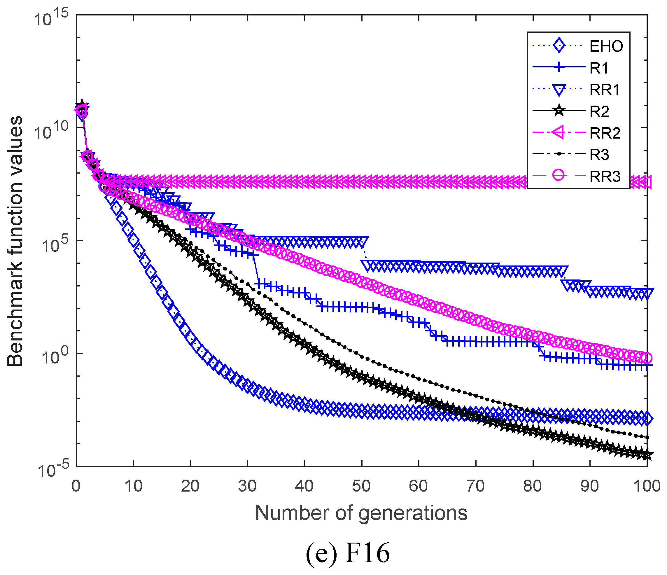
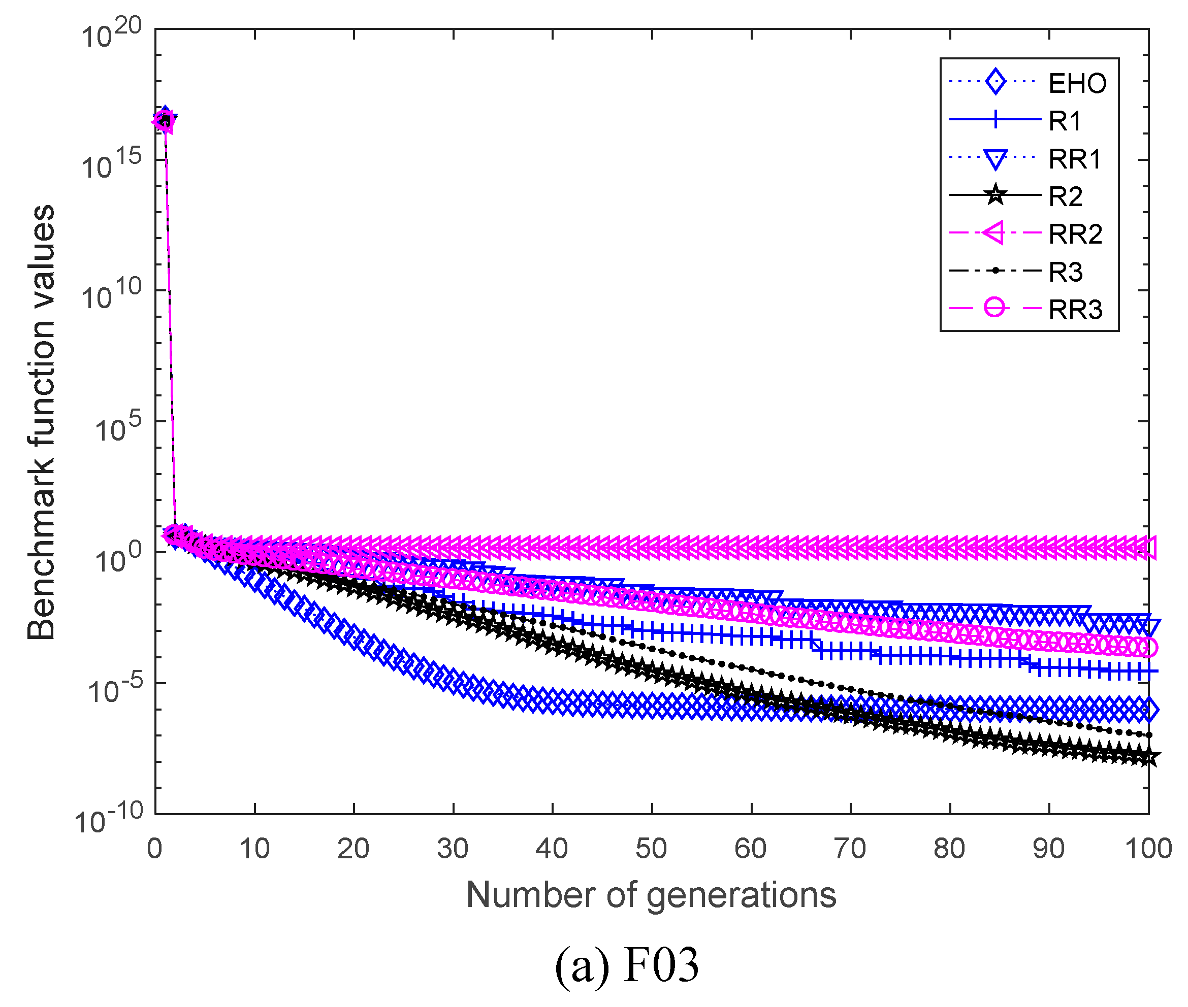
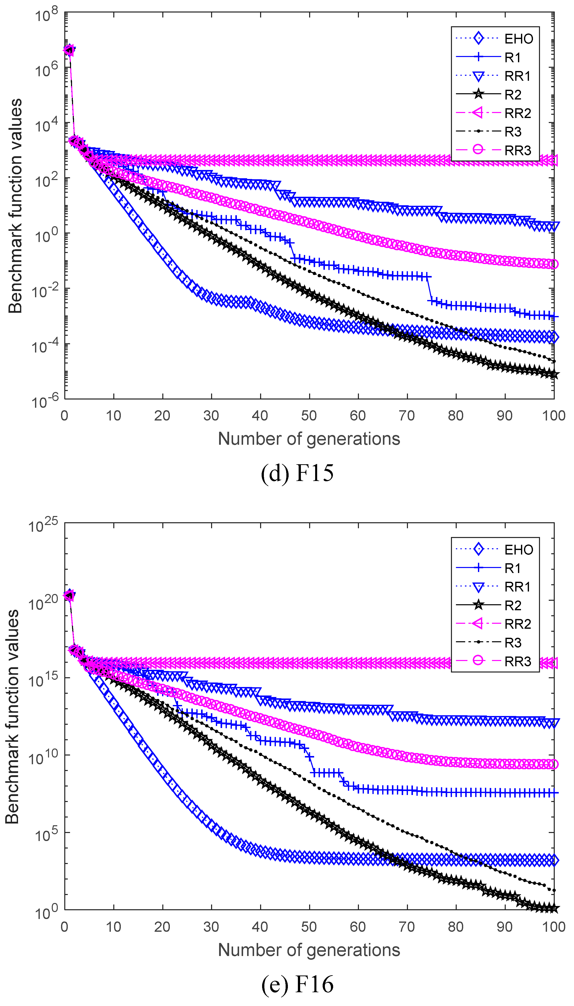
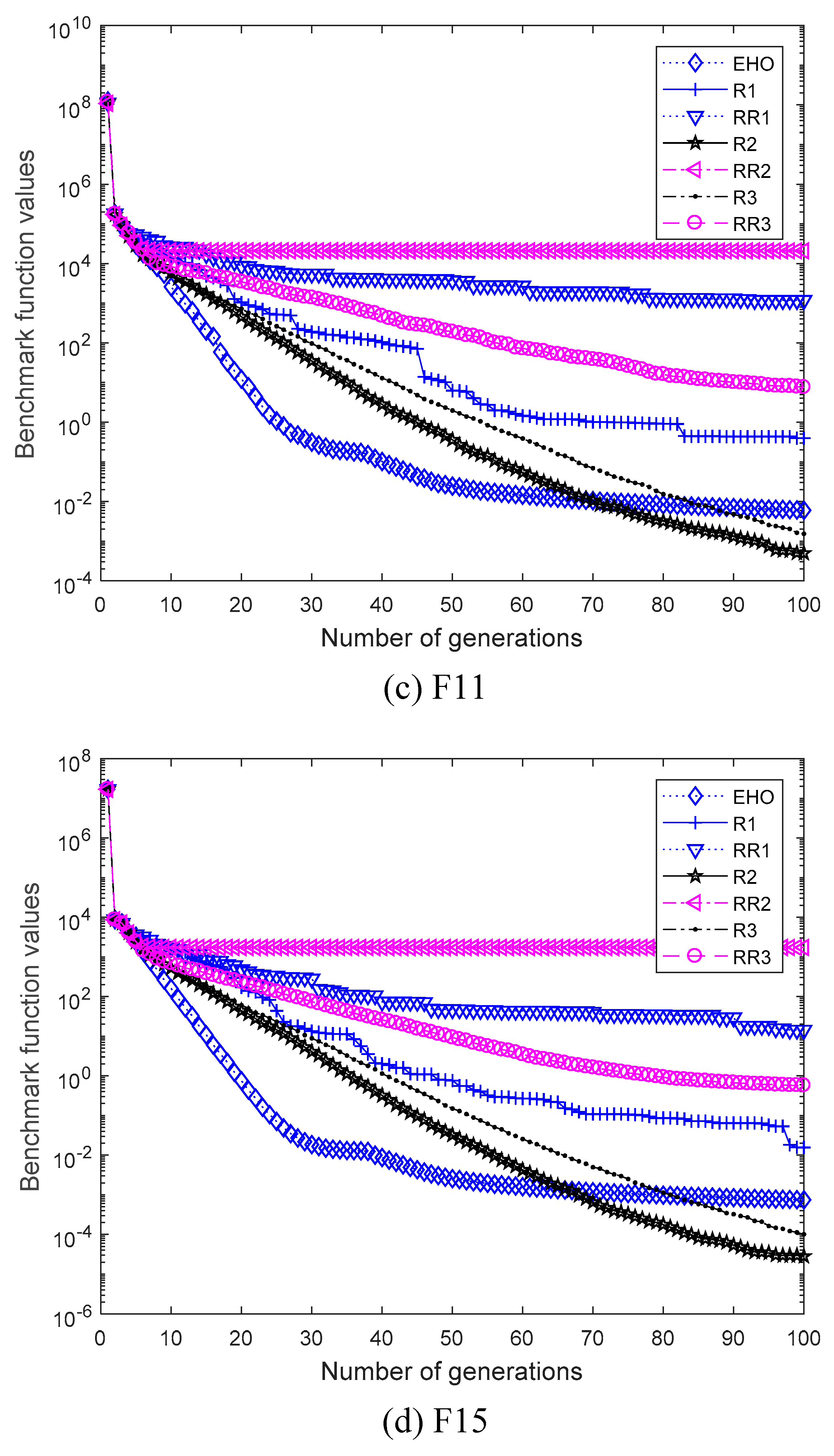
To provide a clear demonstration of the effectiveness of the different individual updating strategies, in this part of our work, we selected five functions randomly from the 16 large-scale complex functions, and their convergence histories with dimension D = 50, 100, 200, 500, and 1000. From Figure 1, Figure 2, Figure 3, Figure 4 and Figure 5, we can see that of the seven metaheuristic algorithms, R2 succeeded in finding the best function values at the end of the search in each of these five large-scale complicated functions. This trend coincided with our previous analysis.
5.2. Constrained Optimization
Besides the standard benchmark evaluation, in this section, fourteen constrained optimization problems originated from CEC 2017 [121] are selected in order to further verify the performance of six improved versions of EHO, namely: EHOR1, EHORR1, EHOR2, EHORR2, EHOR3, and EHORR3. The six variants of the EHO were investigated fully through a series of experiments, using fourteen large-scale constrained benchmarks with dimensions D = 50, and 100. These complicated large-scale benchmarks can be found in Table 13. More information about all of the benchmarks can be found in [86,118,119]. As before, we performed 30 independent runs under the same conditions as shown in the literature [120]. For all of the parameters, they are the same as before.
5.2.1. D = 50
In this section of our work, seven kinds of EHOs were evaluated using the 14 constrained benchmarks mentioned previously, with dimension D = 50. The obtained mean function values and standard values from thirty runs are recorded in Table 14 and Table 15.
From Table 14, we can see that in terms of the mean function values, RR1 performed the best, at a level far better than the other methods. As for the other methods, R1 and R2 provided a similar performance to each other, and they could find the smallest fitness values successfully on two constrained functions. From Table 15, it can be observed that RR3 performed in the most stable way, while for the other algorithms, they have a similar stable performance.
5.2.2. D = 100
As above, the same seven kinds of EHOs were evaluated using the fourteen constrained benchmarks mentioned previously, with dimension D = 100. The obtained mean function values and standard values from 30 runs are recorded in Table 16 and Table 17.
Regarding the mean function values, Table 16 shows that RR1 and R2 have the same performance, which performed much better than the other algorithms, providing the smallest function values on 4 out of 14 functions. As for the other algorithms, R1 ranks R2, EHO, RR2, R3, and RR3 gave a similar performance to each other, performing the best only on one function each. From Table 17, it can be observed that RR3 performed in the most stable way, while for the other algorithms, R1 has a significant advantage over the other algorithms.
6. Conclusions
In optimization research, few metaheuristic algorithms reuse previous information to guide the later updating process. In our proposed improvement for basic elephant herd optimization, the previous information in the population is extracted to guide the later search process. We select one, two, or three elephant individuals from the previous iterations in either a fixed or random manner. Using the information from the selected previous elephant individuals, we offer six individual updating strategies (R1, RR1, R2, RR2, R3, and RR3) that are then incorporated into the basic EHO in order to generate six variants of EHO. The final EHO individual at this iteration is generated according to the individual generated by the basic EHO at the current iteration, along with the selected previous individuals using a weighted sum. The weights are determined by a random number and the fitness of the elephant individuals at the previous iteration.
We tested our six proposed algorithms against 16 large-scale test cases. Among the six individual updating strategies, R2 performed much better than the others on most benchmarks. The experimental results demonstrated that the proposed EHO variations significantly outperformed the basic EHO.
In future research, we will propose more individual updating strategies to further improve the performance of EHO. In addition, the proposed individual updating strategies will be incorporated into other metaheuristic algorithms. We believe they will generate promising results on large-scale test functions and practical engineering cases.
Author Contributions
Methodology, J.L. and Y.L.; software, L.G. and Y.L.; validation, Y.L. and C.L.; formal analysis, J.L., Y.L., and C.L.; supervision, L.G.
Acknowledgments
This work was supported by the Overall Design and Application Framework Technology of Photoelectric System (no. 315090501) and the Early Warning and Laser Jamming System for Low and Slow Targets (no. 20170203015GX).
Conflicts of Interest
The authors declare no conflict of interest.
References
- Wang, G.-G.; Tan, Y. Improving metaheuristic algorithms with information feedback models. IEEE Trans. Cybern. 2019, 49, 542–555. [Google Scholar] [CrossRef] [PubMed]
- Saleh, H.; Nashaat, H.; Saber, W.; Harb, H.M. IPSO task scheduling algorithm for large scale data in cloud computing environment. IEEE Access 2019, 7, 5412–5420. [Google Scholar] [CrossRef]
- Zhang, Y.F.; Chiang, H.D. A novel consensus-based particle swarm optimization-assisted trust-tech methodology for large-scale global optimization. IEEE Trans. Cybern. 2017, 47, 2717–2729. [Google Scholar] [PubMed]
- Kazimipour, B.; Omidvar, M.N.; Qin, A.K.; Li, X.; Yao, X. Bandit-based cooperative coevolution for tackling contribution imbalance in large-scale optimization problems. Appl. Soft Compt. 2019, 76, 265–281. [Google Scholar] [CrossRef]
- Jia, Y.-H.; Zhou, Y.-R.; Lin, Y.; Yu, W.-J.; Gao, Y.; Lu, L. A Distributed Cooperative Co-evolutionary CMA Evolution Strategy for Global Optimization of Large-Scale Overlapping Problems. IEEE Access 2019, 7, 19821–19834. [Google Scholar] [CrossRef]
- De Falco, I.; Della Cioppa, A.; Trunfio, G.A. Investigating surrogate-assisted cooperative coevolution for large-Scale global optimization. Inf. Sci. 2019, 482, 1–26. [Google Scholar] [CrossRef]
- Dhiman, G.; Kumar, V. Seagull optimization algorithm: Theory and its applications for large-scale industrial engineering problems. Knowl.-Based Syst. 2019, 165, 169–196. [Google Scholar] [CrossRef]
- Cravo, G.L.; Amaral, A.R.S. A GRASP algorithm for solving large-scale single row facility layout problems. Comput. Oper. Res. 2019, 106, 49–61. [Google Scholar] [CrossRef]
- Zhao, X.; Liang, J.; Dang, C. A stratified sampling based clustering algorithm for large-scale data. Knowl.-Based Syst. 2019, 163, 416–428. [Google Scholar] [CrossRef]
- Yildiz, Y.E.; Topal, A.O. Large Scale Continuous Global Optimization based on micro Differential Evolution with Local Directional Search. Inf. Sci. 2019, 477, 533–544. [Google Scholar] [CrossRef]
- Ge, Y.F.; Yu, W.J.; Lin, Y.; Gong, Y.J.; Zhan, Z.H.; Chen, W.N.; Zhang, J. Distributed differential evolution based on adaptive mergence and split for large-scale optimization. IEEE Trans. Cybern. 2017. [Google Scholar] [CrossRef]
- Wang, G.-G.; Deb, S.; Coelho, L.d.S. Elephant herding optimization. In Proceedings of the 2015 3rd International Symposium on Computational and Business Intelligence (ISCBI 2015), Bali, Indonesia, 7–9 December 2015; pp. 1–5. [Google Scholar]
- Wang, G.-G.; Deb, S.; Gao, X.-Z.; Coelho, L.d.S. A new metaheuristic optimization algorithm motivated by elephant herding behavior. Int. J. Bio-Inspired Comput. 2016, 8, 394–409. [Google Scholar] [CrossRef]
- Meena, N.K.; Parashar, S.; Swarnkar, A.; Gupta, N.; Niazi, K.R. Improved elephant herding optimization for multiobjective DER accommodation in distribution systems. IEEE Trans. Ind. Inform. 2018, 14, 1029–1039. [Google Scholar] [CrossRef]
- Jayanth, J.; Shalini, V.S.; Ashok Kumar, T.; Koliwad, S. Land-Use/Land-Cover Classification Using Elephant Herding Algorithm. J. Indian Soc. Remote Sens. 2019. [Google Scholar] [CrossRef]
- Rashwan, Y.I.; Elhosseini, M.A.; El Sehiemy, R.A.; Gao, X.Z. On the performance improvement of elephant herding optimization algorithm. Knowl.-Based Syst. 2019. [Google Scholar] [CrossRef]
- Correia, S.D.; Beko, M.; da Silva Cruz, L.A.; Tomic, S. Elephant Herding Optimization for Energy-Based Localization. Sensors 2018, 18, 2849. [Google Scholar]
- Jafari, M.; Salajegheh, E.; Salajegheh, J. An efficient hybrid of elephant herding optimization and cultural algorithm for optimal design of trusses. Eng. Comput.-Ger. 2018. [Google Scholar] [CrossRef]
- Hassanien, A.E.; Kilany, M.; Houssein, E.H.; AlQaheri, H. Intelligent human emotion recognition based on elephant herding optimization tuned support vector regression. Biomed. Signal Process. Control 2018, 45, 182–191. [Google Scholar] [CrossRef]
- Wang, G.-G.; Deb, S.; Cui, Z. Monarch butterfly optimization. Neural Comput. Appl. 2015. [Google Scholar] [CrossRef]
- Yi, J.-H.; Lu, M.; Zhao, X.-J. Quantum inspired monarch butterfly optimization for UCAV path planning navigation problem. Int. J. Bio-Inspired Comput. 2017. Available online: http://www.inderscience.com/info/ingeneral/forthcoming.php?jcode=ijbic (accessed on 30 March 2019).
- Wang, G.-G.; Chu, H.E.; Mirjalili, S. Three-dimensional path planning for UCAV using an improved bat algorithm. Aerosp. Sci. Technol. 2016, 49, 231–238. [Google Scholar] [CrossRef]
- Wang, G.; Guo, L.; Duan, H.; Liu, L.; Wang, H.; Shao, M. Path planning for uninhabited combat aerial vehicle using hybrid meta-heuristic DE/BBO algorithm. Adv. Sci. Eng. Med. 2012, 4, 550–564. [Google Scholar] [CrossRef]
- Feng, Y.; Wang, G.-G.; Deb, S.; Lu, M.; Zhao, X. Solving 0-1 knapsack problem by a novel binary monarch butterfly optimization. Neural Comput. Appl. 2017, 28, 1619–1634. [Google Scholar] [CrossRef]
- Feng, Y.; Yang, J.; Wu, C.; Lu, M.; Zhao, X.-J. Solving 0-1 knapsack problems by chaotic monarch butterfly optimization algorithm. Memetic Comput. 2018, 10, 135–150. [Google Scholar] [CrossRef]
- Feng, Y.; Wang, G.-G.; Li, W.; Li, N. Multi-strategy monarch butterfly optimization algorithm for discounted {0-1} knapsack problem. Neural Comput. Appl. 2018, 30, 3019–3036. [Google Scholar] [CrossRef]
- Feng, Y.; Yang, J.; He, Y.; Wang, G.-G. Monarch butterfly optimization algorithm with differential evolution for the discounted {0-1} knapsack problem. Acta Electron. Sin. 2018, 46, 1343–1350. [Google Scholar]
- Feng, Y.; Wang, G.-G.; Dong, J.; Wang, L. Opposition-based learning monarch butterfly optimization with Gaussian perturbation for large-scale 0-1 knapsack problem. Comput. Electr. Eng. 2018, 67, 454–468. [Google Scholar] [CrossRef]
- Wang, G.-G.; Zhao, X.; Deb, S. A novel monarch butterfly optimization with greedy strategy and self-adaptive crossover operator. In Proceedings of the 2015 2nd International Conference on Soft Computing & Machine Intelligence (ISCMI 2015), Hong Kong, 23–24 November 2015; pp. 45–50. [Google Scholar]
- Wang, G.-G.; Deb, S.; Zhao, X.; Cui, Z. A new monarch butterfly optimization with an improved crossover operator. Oper. Res. Int. J. 2018, 18, 731–755. [Google Scholar] [CrossRef]
- Wang, G.-G.; Hao, G.-S.; Cheng, S.; Qin, Q. A discrete monarch butterfly optimization for Chinese TSP problem. In Proceedings of the Advances in Swarm Intelligence: 7th International Conference, ICSI 2016, Part I, Bali, Indonesia, 25–30 June 2016; Tan, Y., Shi, Y., Niu, B., Eds.; Springer International Publishing: Cham, Switzerland, 2016; Volume 9712, pp. 165–173. [Google Scholar]
- Wang, G.-G.; Hao, G.-S.; Cheng, S.; Cui, Z. An improved monarch butterfly optimization with equal partition and F/T mutation. In Proceedings of the Eight International Conference on Swarm Intelligence (ICSI 2017), Fukuoka, Japan, 27 July–1 August 2017; pp. 106–115. [Google Scholar]
- Wang, G.-G. Moth search algorithm: A bio-inspired metaheuristic algorithm for global optimization problems. Memetic Comput. 2018, 10, 151–164. [Google Scholar] [CrossRef]
- Feng, Y.; An, H.; Gao, X. The importance of transfer function in solving set-union knapsack problem based on discrete moth search algorithm. Mathematics 2019, 7, 17. [Google Scholar] [CrossRef]
- Elaziz, M.A.; Xiong, S.; Jayasena, K.P.N.; Li, L. Task scheduling in cloud computing based on hybrid moth search algorithm and differential evolution. Knowl.-Based Syst. 2019. [Google Scholar] [CrossRef]
- Feng, Y.; Wang, G.-G. Binary moth search algorithm for discounted {0-1} knapsack problem. IEEE Access 2018, 6, 10708–10719. [Google Scholar] [CrossRef]
- Gandomi, A.H.; Alavi, A.H. Krill herd: A new bio-inspired optimization algorithm. Commun. Nonlinear Sci. Numer. Simulat. 2012, 17, 4831–4845. [Google Scholar] [CrossRef]
- Wang, G.-G.; Gandomi, A.H.; Alavi, A.H.; Hao, G.-S. Hybrid krill herd algorithm with differential evolution for global numerical optimization. Neural Comput. Appl. 2014, 25, 297–308. [Google Scholar] [CrossRef]
- Wang, G.-G.; Gandomi, A.H.; Alavi, A.H. Stud krill herd algorithm. Neurocomputing 2014, 128, 363–370. [Google Scholar] [CrossRef]
- Wang, G.-G.; Gandomi, A.H.; Alavi, A.H. An effective krill herd algorithm with migration operator in biogeography-based optimization. Appl. Math. Model. 2014, 38, 2454–2462. [Google Scholar] [CrossRef]
- Guo, L.; Wang, G.-G.; Gandomi, A.H.; Alavi, A.H.; Duan, H. A new improved krill herd algorithm for global numerical optimization. Neurocomputing 2014, 138, 392–402. [Google Scholar] [CrossRef]
- Wang, G.-G.; Deb, S.; Gandomi, A.H.; Alavi, A.H. Opposition-based krill herd algorithm with Cauchy mutation and position clamping. Neurocomputing 2016, 177, 147–157. [Google Scholar] [CrossRef]
- Wang, G.-G.; Gandomi, A.H.; Alavi, A.H.; Deb, S. A hybrid method based on krill herd and quantum-behaved particle swarm optimization. Neural Comput. Appl. 2016, 27, 989–1006. [Google Scholar] [CrossRef]
- Wang, G.-G.; Gandomi, A.H.; Yang, X.-S.; Alavi, A.H. A new hybrid method based on krill herd and cuckoo search for global optimization tasks. Int. J. Bio-Inspired Comput. 2016, 8, 286–299. [Google Scholar] [CrossRef]
- Abdel-Basset, M.; Wang, G.-G.; Sangaiah, A.K.; Rushdy, E. Krill herd algorithm based on cuckoo search for solving engineering optimization problems. Multimed. Tools Appl. 2017. [Google Scholar] [CrossRef]
- Wang, G.-G.; Gandomi, A.H.; Alavi, A.H.; Deb, S. A multi-stage krill herd algorithm for global numerical optimization. Int. J. Artif. Intell. Tools 2016, 25, 1550030. [Google Scholar] [CrossRef]
- Wang, G.-G.; Gandomi, A.H.; Alavi, A.H.; Gong, D. A comprehensive review of krill herd algorithm: Variants, hybrids and applications. Artif. Intell. Rev. 2019, 51, 119–148. [Google Scholar] [CrossRef]
- Karaboga, D.; Basturk, B. A powerful and efficient algorithm for numerical function optimization: Artificial bee colony (ABC) algorithm. J. Glob. Optim. 2007, 39, 459–471. [Google Scholar] [CrossRef]
- Wang, H.; Yi, J.-H. An improved optimization method based on krill herd and artificial bee colony with information exchange. Memetic Comput. 2018, 10, 177–198. [Google Scholar] [CrossRef]
- Liu, F.; Sun, Y.; Wang, G.-G.; Wu, T. An artificial bee colony algorithm based on dynamic penalty and chaos search for constrained optimization problems. Arab. J. Sci. Eng. 2018, 43, 7189–7208. [Google Scholar] [CrossRef]
- Kennedy, J.; Eberhart, R. Particle swarm optimization. In Proceedings of the IEEE International Conference on Neural Networks, Perth, Australia, 27 November–1 December 1995; pp. 1942–1948. [Google Scholar]
- Helwig, S.; Branke, J.; Mostaghim, S. Experimental analysis of bound handling techniques in particle swarm optimization. IEEE Trans. Evol. Comput. 2012, 17, 259–271. [Google Scholar] [CrossRef]
- Li, J.; Zhang, J.; Jiang, C.; Zhou, M. Composite particle swarm optimizer with historical memory for function optimization. IEEE Trans. Cybern. 2015, 45, 2350–2363. [Google Scholar] [CrossRef]
- Gong, M.; Cai, Q.; Chen, X.; Ma, L. Complex network clustering by multiobjective discrete particle swarm optimization based on decomposition. IEEE Trans. Evol. Comput. 2014, 18, 82–97. [Google Scholar] [CrossRef]
- Yuan, Y.; Ji, B.; Yuan, X.; Huang, Y. Lockage scheduling of Three Gorges-Gezhouba dams by hybrid of chaotic particle swarm optimization and heuristic-adjusted strategies. Appl. Math. Comput. 2015, 270, 74–89. [Google Scholar] [CrossRef]
- Zhang, Y.; Gong, D.W.; Cheng, J. Multi-objective particle swarm optimization approach for cost-based feature selection in classification. IEEE/ACM Trans. Comput. Biol. Bioinform. 2017, 14, 64–75. [Google Scholar] [CrossRef]
- Yang, X.-S.; Deb, S. Cuckoo search via Lévy flights. In Proceedings of the World Congress on Nature & Biologically Inspired Computing (NaBIC 2009), Coimbatore, India, 9–11 December 2009; pp. 210–214. [Google Scholar]
- Wang, G.-G.; Gandomi, A.H.; Zhao, X.; Chu, H.E. Hybridizing harmony search algorithm with cuckoo search for global numerical optimization. Soft Comput. 2016, 20, 273–285. [Google Scholar] [CrossRef]
- Wang, G.-G.; Deb, S.; Gandomi, A.H.; Zhang, Z.; Alavi, A.H. Chaotic cuckoo search. Soft Comput. 2016, 20, 3349–3362. [Google Scholar] [CrossRef]
- Cui, Z.; Sun, B.; Wang, G.-G.; Xue, Y.; Chen, J. A novel oriented cuckoo search algorithm to improve DV-Hop performance for cyber-physical systems. J. Parallel Distrib. Comput. 2017, 103, 42–52. [Google Scholar] [CrossRef]
- Li, J.; Li, Y.-X.; Tian, S.-S.; Zou, J. Dynamic cuckoo search algorithm based on Taguchi opposition-based search. Int. J. Bio-Inspired Comput. 2019, 13, 59–69. [Google Scholar] [CrossRef]
- Baluja, S. Population-Based Incremental Learning: A Method for Integrating Genetic Search Based Function Optimization and Competitive Learning; CMU-CS-94-163; Carnegie Mellon University: Pittsburgh, PA, USA, 1994. [Google Scholar]
- Storn, R.; Price, K. Differential evolution-a simple and efficient heuristic for global optimization over continuous spaces. J. Glob. Optim. 1997, 11, 341–359. [Google Scholar] [CrossRef]
- Das, S.; Suganthan, P.N. Differential evolution: A survey of the state-of-the-art. IEEE Trans. Evol. Comput. 2011, 15, 4–31. [Google Scholar] [CrossRef]
- Li, Y.-L.; Zhan, Z.-H.; Gong, Y.-J.; Chen, W.-N.; Zhang, J.; Li, Y. Differential evolution with an evolution path: A deep evolutionary algorithm. IEEE Trans. Cybern. 2015, 45, 1798–1810. [Google Scholar] [CrossRef] [PubMed]
- Teoh, B.E.; Ponnambalam, S.G.; Kanagaraj, G. Differential evolution algorithm with local search for capacitated vehicle routing problem. Int. J. Bio-Inspired Comput. 2015, 7, 321–342. [Google Scholar] [CrossRef]
- Beyer, H.; Schwefel, H. Natural Computing; Kluwer Academic Publishers: Dordrecht, The Netherlands, 2002. [Google Scholar]
- Reddy, S.S.; Panigrahi, B.; Debchoudhury, S.; Kundu, R.; Mukherjee, R. Short-term hydro-thermal scheduling using CMA-ES with directed target to best perturbation scheme. Int. J. Bio-Inspired Comput. 2015, 7, 195–208. [Google Scholar] [CrossRef]
- Gandomi, A.H.; Yang, X.-S.; Alavi, A.H. Mixed variable structural optimization using firefly algorithm. Comput. Struct. 2011, 89, 2325–2336. [Google Scholar] [CrossRef]
- Yang, X.S. Firefly algorithm, stochastic test functions and design optimisation. Int. J. Bio-Inspired Comput. 2010, 2, 78–84. [Google Scholar] [CrossRef]
- Wang, G.-G.; Guo, L.; Duan, H.; Wang, H. A new improved firefly algorithm for global numerical optimization. J. Comput. Theor. Nanosci. 2014, 11, 477–485. [Google Scholar] [CrossRef]
- Zhang, Y.; Song, X.-F.; Gong, D.-W. A return-cost-based binary firefly algorithm for feature selection. Inf. Sci. 2017, 418–419, 561–574. [Google Scholar] [CrossRef]
- Wang, G.-G.; Deb, S.; Coelho, L.d.S. Earthworm optimization algorithm: A bio-inspired metaheuristic algorithm for global optimization problems. Int. J. Bio-Inspired Comput. 2018, 12, 1–23. [Google Scholar] [CrossRef]
- Goldberg, D.E. Genetic Algorithms in Search, Optimization and Machine Learning; Addison-Wesley: New York, NY, USA, 1998. [Google Scholar]
- Sun, X.; Gong, D.; Jin, Y.; Chen, S. A new surrogate-assisted interactive genetic algorithm with weighted semisupervised learning. IEEE Trans. Cybern. 2013, 43, 685–698. [Google Scholar] [PubMed]
- Garg, H. A hybrid PSO-GA algorithm for constrained optimization problems. Appl. Math. Comput. 2016, 274, 292–305. [Google Scholar] [CrossRef]
- Dorigo, M.; Stutzle, T. Ant Colony Optimization; MIT Press: Cambridge, MA, USA, 2004. [Google Scholar]
- Ciornei, I.; Kyriakides, E. Hybrid ant colony-genetic algorithm (GAAPI) for global continuous optimization. IEEE Trans. Syst. Man Cybern. Part B Cybern. 2012, 42, 234–245. [Google Scholar] [CrossRef] [PubMed]
- Sun, X.; Zhang, Y.; Ren, X.; Chen, K. Optimization deployment of wireless sensor networks based on culture-ant colony algorithm. Appl. Math. Comput. 2015, 250, 58–70. [Google Scholar] [CrossRef]
- Wang, G.-G.; Guo, L.; Gandomi, A.H.; Hao, G.-S.; Wang, H. Chaotic Krill Herd algorithm. Inf. Sci. 2014, 274, 17–34. [Google Scholar] [CrossRef]
- Li, J.; Tang, Y.; Hua, C.; Guan, X. An improved krill herd algorithm: Krill herd with linear decreasing step. Appl. Math. Comput. 2014, 234, 356–367. [Google Scholar] [CrossRef]
- Mehrabian, A.R.; Lucas, C. A novel numerical optimization algorithm inspired from weed colonization. Ecol. Inform. 2006, 1, 355–366. [Google Scholar] [CrossRef]
- Sang, H.-Y.; Duan, P.-Y.; Li, J.-Q. An effective invasive weed optimization algorithm for scheduling semiconductor final testing problem. Swarm Evol. Comput. 2018, 38, 42–53. [Google Scholar] [CrossRef]
- Sang, H.-Y.; Pan, Q.-K.; Duan, P.-Y.; Li, J.-Q. An effective discrete invasive weed optimization algorithm for lot-streaming flowshop scheduling problems. J. Intell. Manuf. 2015, 29, 1337–1349. [Google Scholar] [CrossRef]
- Khatib, W.; Fleming, P. The stud GA: A mini revolution? In Proceedings of the 5th International Conference on Parallel Problem Solving from Nature, New York, NY, USA, 27–30 September 1998; pp. 683–691. [Google Scholar]
- Simon, D. Biogeography-based optimization. IEEE Trans. Evol. Comput. 2008, 12, 702–713. [Google Scholar] [CrossRef]
- Simon, D.; Ergezer, M.; Du, D.; Rarick, R. Markov models for biogeography-based optimization. IEEE Trans. Syst. Man Cybern. Part B Cybern. 2011, 41, 299–306. [Google Scholar] [CrossRef]
- Geem, Z.W.; Kim, J.H.; Loganathan, G.V. A new heuristic optimization algorithm: Harmony search. Simulation 2001, 76, 60–68. [Google Scholar] [CrossRef]
- Bilbao, M.N.; Ser, J.D.; Salcedo-Sanz, S.; Casanova-Mateo, C. On the application of multi-objective harmony search heuristics to the predictive deployment of firefighting aircrafts: A realistic case study. Int. J. Bio-Inspired Comput. 2015, 7, 270–284. [Google Scholar] [CrossRef]
- Amaya, I.; Correa, R. Finding resonant frequencies of microwave cavities through a modified harmony search algorithm. Int. J. Bio-Inspired Comput. 2015, 7, 285–295. [Google Scholar] [CrossRef]
- Yang, X.S.; Gandomi, A.H. Bat algorithm: A novel approach for global engineering optimization. Eng. Comput. 2012, 29, 464–483. [Google Scholar] [CrossRef]
- Xue, F.; Cai, Y.; Cao, Y.; Cui, Z.; Li, F. Optimal parameter settings for bat algorithm. Int. J. Bio-Inspired Comput. 2015, 7, 125–128. [Google Scholar] [CrossRef]
- Wu, G.; Shen, X.; Li, H.; Chen, H.; Lin, A.; Suganthan, P.N. Ensemble of differential evolution variants. Inf. Sci. 2018, 423, 172–186. [Google Scholar] [CrossRef]
- Wang, G.-G.; Lu, M.; Zhao, X.-J. An improved bat algorithm with variable neighborhood search for global optimization. In Proceedings of the 2016 IEEE Congress on Evolutionary Computation (IEEE CEC 2016), Vancouver, BC, Canada, 25–29 July 2016; pp. 1773–1778. [Google Scholar]
- Duan, H.; Zhao, W.; Wang, G.; Feng, X. Test-sheet composition using analytic hierarchy process and hybrid metaheuristic algorithm TS/BBO. Math. Probl. Eng. 2012, 2012, 712752. [Google Scholar] [CrossRef]
- Pan, Q.-K.; Gao, L.; Wang, L.; Liang, J.; Li, X.-Y. Effective heuristics and metaheuristics to minimize total flowtime for the distributed permutation flowshop problem. Expert Syst. Appl. 2019. [Google Scholar] [CrossRef]
- Peng, K.; Pan, Q.-K.; Gao, L.; Li, X.; Das, S.; Zhang, B. A multi-start variable neighbourhood descent algorithm for hybrid flowshop rescheduling. Swarm Evol. Comput. 2019, 45, 92–112. [Google Scholar] [CrossRef]
- Zhang, Y.; Gong, D.; Hu, Y.; Zhang, W. Feature selection algorithm based on bare bones particle swarm optimization. Neurocomputing 2015, 148, 150–157. [Google Scholar] [CrossRef]
- Zhang, Y.; Gong, D.-W.; Sun, J.-Y.; Qu, B.-Y. A decomposition-based archiving approach for multi-objective evolutionary optimization. Inf. Sci. 2018, 430–431, 397–413. [Google Scholar] [CrossRef]
- Logesh, R.; Subramaniyaswamy, V.; Vijayakumar, V.; Gao, X.-Z.; Wang, G.-G. Hybrid bio-inspired user clustering for the generation of diversified recommendations. Neural Comput. Appl. 2019. [Google Scholar] [CrossRef]
- Wang, G.-G.; Cai, X.; Cui, Z.; Min, G.; Chen, J. High performance computing for cyber physical social systems by using evolutionary multi-objective optimization algorithm. IEEE Trans. Emerg. Top. Comput. 2017. [Google Scholar] [CrossRef]
- Zou, D.; Li, S.; Wang, G.-G.; Li, Z.; Ouyang, H. An improved differential evolution algorithm for the economic load dispatch problems with or without valve-point effects. Appl. Energ. 2016, 181, 375–390. [Google Scholar] [CrossRef]
- Rizk-Allah, R.M.; El-Sehiemy, R.A.; Wang, G.-G. A novel parallel hurricane optimization algorithm for secure emission/economic load dispatch solution. Appl. Soft Compt. 2018, 63, 206–222. [Google Scholar] [CrossRef]
- Yi, J.-H.; Wang, J.; Wang, G.-G. Improved probabilistic neural networks with self-adaptive strategies for transformer fault diagnosis problem. Adv. Mech. Eng. 2016, 8, 1687814015624832. [Google Scholar] [CrossRef]
- Sang, H.-Y.; Pan, Q.-K.; Li, J.-Q.; Wang, P.; Han, Y.-Y.; Gao, K.-Z.; Duan, P. Effective invasive weed optimization algorithms for distributed assembly permutation flowshop problem with total flowtime criterion. Swarm Evol. Comput. 2019, 44, 64–73. [Google Scholar] [CrossRef]
- Yi, J.-H.; Xing, L.-N.; Wang, G.-G.; Dong, J.; Vasilakos, A.V.; Alavi, A.H.; Wang, L. Behavior of crossover operators in NSGA-III for large-scale optimization problems. Inf. Sci. 2018. [Google Scholar] [CrossRef]
- Yi, J.-H.; Deb, S.; Dong, J.; Alavi, A.H.; Wang, G.-G. An improved NSGA-III Algorithm with adaptive mutation operator for big data optimization problems. Future Gener. Comput. Syst. 2018, 88, 571–585. [Google Scholar] [CrossRef]
- Liu, K.; Gong, D.; Meng, F.; Chen, H.; Wang, G.-G. Gesture segmentation based on a two-phase estimation of distribution algorithm. Inf. Sci. 2017, 394–395, 88–105. [Google Scholar] [CrossRef]
- Wang, G.-G.; Guo, L.; Duan, H.; Liu, L.; Wang, H. The model and algorithm for the target threat assessment based on Elman_AdaBoost strong predictor. Acta Electron. Sin. 2012, 40, 901–906. [Google Scholar]
- Wang, G.; Guo, L.; Duan, H. Wavelet neural network using multiple wavelet functions in target threat assessment. Sci. World J. 2013, 2013, 632437. [Google Scholar] [CrossRef] [PubMed]
- Nan, X.; Bao, L.; Zhao, X.; Zhao, X.; Sangaiah, A.K.; Wang, G.-G.; Ma, Z. EPuL: An enhanced positive-unlabeled learning algorithm for the prediction of pupylation sites. Molecules 2017, 22, 1463. [Google Scholar] [CrossRef] [PubMed]
- Zou, D.-X.; Deb, S.; Wang, G.-G. Solving IIR system identification by a variant of particle swarm optimization. Neural Comput. Appl. 2018, 30, 685–698. [Google Scholar] [CrossRef]
- Rizk-Allah, R.M.; El-Sehiemy, R.A.; Deb, S.; Wang, G.-G. A novel fruit fly framework for multi-objective shape design of tubular linear synchronous motor. J. Supercomput. 2017, 73, 1235–1256. [Google Scholar] [CrossRef]
- Sun, J.; Gong, D.; Li, J.; Wang, G.-G.; Zeng, X.-J. Interval multi-objective optimization with memetic algorithms. IEEE Trans. Cybern. 2019. [Google Scholar] [CrossRef] [PubMed]
- Liu, Y.; Gong, D.; Sun, X.; Zhang, Y. Many-objective evolutionary optimization based on reference points. Appl. Soft Compt. 2017, 50, 344–355. [Google Scholar] [CrossRef]
- Gong, D.; Liu, Y.; Yen, G.G. A Meta-Objective Approach for Many-Objective Evolutionary Optimization. Evol. Comput. 2018. [Google Scholar] [CrossRef]
- Gong, D.; Sun, J.; Miao, Z. A set-based genetic algorithm for interval many-objective optimization problems. IEEE Trans. Evol. Comput. 2018, 22, 47–60. [Google Scholar] [CrossRef]
- Yao, X.; Liu, Y.; Lin, G. Evolutionary programming made faster. IEEE Trans. Evol. Comput. 1999, 3, 82–102. [Google Scholar]
- Yang, X.-S.; Cui, Z.; Xiao, R.; Gandomi, A.H.; Karamanoglu, M. Swarm Intelligence and Bio-Inspired Computation; Elsevier: Waltham, MA, USA, 2013. [Google Scholar]
- Wang, G.; Guo, L.; Wang, H.; Duan, H.; Liu, L.; Li, J. Incorporating mutation scheme into krill herd algorithm for global numerical optimization. Neural Comput. Appl. 2014, 24, 853–871. [Google Scholar] [CrossRef]
- Wu, G.; Mallipeddi, R.; Suganthan, P.N. Problem Definitions and Evaluation Criteria for the CEC 2017 Competition on Constrained Real-Parameter Optimization; National University of Defense Technology: Changsha, China; Kyungpook National University: Daegu, Korea; Nanyang Technological University: Singapore, 2017. [Google Scholar]
Figure 1.
Optimization process of seven algorithms on five functions with D = 50. EHO—elephant herd optimization.
Figure 1.
Optimization process of seven algorithms on five functions with D = 50. EHO—elephant herd optimization.


Figure 2.
Optimization process of seven algorithms on five functions with D = 100.


Figure 3.
Optimization process of seven algorithms on five functions with D = 200.


Figure 4.
Optimization process of seven algorithms on five functions with D = 500.


Figure 5.
Optimization process of seven algorithms on five functions with D = 1000.


Table 1.
Sixteen benchmark functions.
| No. | Name | No. | Name |
|---|---|---|---|
| F01 | Ackley | F09 | Rastrigin |
| F02 | Alpine | F10 | Schwefel 2.26 |
| F03 | Brown | F11 | Schwefel 1.2 |
| F04 | Holzman 2 function | F12 | Schwefel 2.22 |
| F05 | Levy | F13 | Schwefel 2.21 |
| F06 | Penalty #1 | F14 | Sphere |
| F07 | Powell | F15 | Sum function |
| F08 | Quartic with noise | F16 | Zakharov |
Table 2.
Mean function values obtained by elephant herd optimization (EHO) and six improved methods with D = 50.
Table 2.
Mean function values obtained by elephant herd optimization (EHO) and six improved methods with D = 50.
| EHO | R1 | RR1 | R2 | RR2 | R3 | RR3 | |
|---|---|---|---|---|---|---|---|
| F01 | 2.57 × 10⁻⁴ | 7.11 × 10⁻⁴ | 0.05 | 8.38 × 10⁻⁵ | 1.57 | 1.53 × 10⁻⁴ | 0.01 |
| F02 | 1.04 × 10⁻⁴ | 2.69 × 10⁻⁴ | 0.01 | 2.74 × 10⁻⁵ | 0.23 | 5.13 × 10⁻⁵ | 2.38 × 10⁻³ |
| F03 | 4.41 × 10⁻⁷ | 9.16 × 10⁻⁶ | 3.37 × 10⁻³ | 6.14 × 10⁻⁹ | 0.76 | 4.32 × 10⁻⁸ | 8.25 × 10⁻⁵ |
| F04 | 1.50 × 10⁻¹⁵ | 4.97 × 10⁻¹¹ | 3.58 × 10⁻⁶ | 2.27 × 10⁻¹⁶ | 0.03 | 3.38 × 10⁻¹⁶ | 1.82 × 10⁻⁹ |
| F05 | 4.49 | 4.25 | 3.95 | 4.43 | 4.89 | 4.44 | 4.50 |
| F06 | 1.22 | 1.06 | 1.62 | 1.72 | 2.01 | 1.76 | 1.79 |
| F07 | 5.13 × 10⁻⁷ | 2.55 × 10⁻⁶ | 0.02 | 3.50 × 10⁻⁸ | 2.25 | 1.51 × 10⁻⁷ | 4.85 × 10⁻⁴ |
| F08 | 2.57 × 10⁻¹⁶ | 1.24 × 10⁻¹⁵ | 7.23 × 10⁻⁹ | 2.21 × 10⁻¹⁶ | 1.72 × 10⁻⁵ | 2.21 × 10⁻¹⁶ | 4.03 × 10⁻¹³ |
| F09 | 2.59 × 10⁻⁶ | 6.86 × 10⁻⁵ | 0.03 | 9.83 × 10⁻⁸ | 9.28 | 5.06 × 10⁻⁷ | 3.92 × 10⁻³ |
| F10 | 1.65 × 10⁴ | 1.64 × 10⁴ | 1.63 × 10⁴ | 1.65 × 10⁴ | 1.61 × 10⁴ | 1.64 × 10⁴ | 1.64 × 10⁴ |
| F11 | 1.44 × 10⁻⁵ | 4.47 × 10⁻⁴ | 0.36 | 1.02 × 10⁻⁶ | 49.04 | 3.52 × 10⁻⁶ | 2.18 |
| F12 | 1.07 × 10⁻³ | 3.81 × 10⁻³ | 0.14 | 2.96 × 10⁻⁴ | 2.37 | 5.31 × 10⁻⁴ | 0.02 |
| F13 | 6.69 × 10⁻⁴ | 1.34 × 10⁻³ | 0.07 | 1.52 × 10⁻⁴ | 1.21 | 3.05 × 10⁻⁴ | 0.01 |
| F14 | 1.27 × 10⁻⁸ | 1.63 × 10⁻⁷ | 3.85 × 10⁻⁴ | 7.00 × 10⁻¹⁰ | 0.04 | 2.50 × 10⁻⁹ | 3.02 × 10⁻⁶ |
| F15 | 6.70 × 10⁻⁷ | 1.40 × 10⁻⁵ | 7.03 × 10⁻³ | 4.76 × 10⁻⁸ | 3.61 | 1.77 × 10⁻⁷ | 9.87 × 10⁻⁴ |
| F16 | 1.28 × 10⁻³ | 0.30 | 512.90 | 3.00 × 10⁻⁵ | 3.87 × 10⁷ | 1.71 × 10⁻⁴ | 0.56 |
| TOTAL | 0 | 1 | 1 | 14 | 0 | 0 | 0 |
Table 3.
Standard values obtained by EHO and six improved methods with D = 50.
| EHO | R1 | RR1 | R2 | RR2 | R3 | RR3 | |
|---|---|---|---|---|---|---|---|
| F01 | 2.39 × 10⁻⁵ | 9.89 × 10⁻⁴ | 0.06 | 3.60 × 10⁻⁵ | 0.22 | 4.89 × 10⁻⁵ | 0.01 |
| F02 | 1.37 × 10⁻⁵ | 3.32 × 10⁻⁴ | 0.01 | 1.14 × 10⁻⁵ | 0.04 | 1.38 × 10⁻⁵ | 2.17 × 10⁻³ |
| F03 | 1.55 × 10⁻⁸ | 3.34 × 10⁻⁵ | 6.16 × 10⁻³ | 3.72 × 10⁻⁹ | 0.07 | 3.52 × 10⁻⁸ | 7.80 × 10⁻⁵ |
| F04 | 4.50 × 10⁻¹⁶ | 2.49 × 10⁻¹⁰ | 1.08 × 10⁻⁵ | 6.72 × 10⁻¹⁸ | 0.01 | 2.92 × 10⁻¹⁶ | 5.64 × 10⁻⁹ |
| F05 | 0.16 | 0.26 | 0.52 | 0.30 | 0.20 | 0.30 | 0.33 |
| F06 | 0.23 | 0.18 | 0.41 | 0.28 | 0.32 | 0.25 | 0.27 |
| F07 | 1.40 × 10⁻⁷ | 5.25 × 10⁻⁶ | 0.04 | 2.71 × 10⁻⁸ | 0.76 | 7.78 × 10⁻⁸ | 1.58 × 10⁻³ |
| F08 | 6.86 × 10⁻¹⁸ | 3.99 × 10⁻¹⁵ | 1.96 × 10⁻⁸ | 1.68 × 10⁻²⁰ | 6.10 × 10⁻⁶ | 1.26 × 10⁻¹⁹ | 1.17 × 10⁻¹² |
| F09 | 4.61 × 10⁻⁷ | 1.75 × 10⁻⁴ | 0.09 | 6.36 × 10⁻⁸ | 1.60 | 3.11 × 10⁻⁷ | 0.02 |
| F10 | 444.40 | 591.40 | 502.50 | 506.70 | 486.40 | 454.70 | 349.00 |
| F11 | 3.73 × 10⁻⁶ | 1.98 × 10⁻³ | 0.71 | 8.92 × 10⁻⁷ | 29.12 | 2.30 × 10⁻⁶ | 9.49 |
| F12 | 1.03 × 10⁻⁴ | 5.54 × 10⁻³ | 0.15 | 1.03 × 10⁻⁴ | 0.28 | 1.21 × 10⁻⁴ | 0.01 |
| F13 | 9.58 × 10⁻⁵ | 1.97 × 10⁻³ | 0.07 | 5.39 × 10⁻⁵ | 0.15 | 6.84 × 10⁻⁵ | 6.05 × 10⁻³ |
| F14 | 2.07 × 10⁻⁹ | 5.02 × 10⁻⁷ | 1.09 × 10⁻³ | 6.10 × 10⁻¹⁰ | 0.01 | 2.04 × 10⁻⁹ | 3.90 × 10⁻⁶ |
| F15 | 1.00 × 10⁻⁷ | 4.76 × 10⁻⁵ | 0.02 | 3.41 × 10⁻⁸ | 0.73 | 8.84 × 10⁻⁸ | 3.40 × 10⁻³ |
| F16 | 8.21 × 10⁻⁴ | 1.43 | 1.23 × 10³ | 2.06 × 10⁻⁵ | 1.92 × 10⁷ | 1.21 × 10⁻⁴ | 0.44 |
| TOTAL | 3 | 1 | 0 | 11 | 0 | 0 | 1 |
Table 4.
Mean function values obtained by EHO and six improved methods with D = 100.
| EHO | R1 | RR1 | R2 | RR2 | R3 | RR3 | |
|---|---|---|---|---|---|---|---|
| F01 | 3.22 × 10⁻⁴ | 6.27 × 10⁻⁴ | 0.12 | 6.92 × 10⁻⁵ | 1.70 | 1.78 × 10⁻⁴ | 0.01 |
| F02 | 2.55 × 10⁻⁴ | 6.86 × 10⁻⁴ | 0.04 | 6.28 × 10⁻⁵ | 0.48 | 1.08 × 10⁻⁴ | 4.78 × 10⁻³ |
| F03 | 9.83 × 10⁻⁷ | 2.65 × 10⁻⁵ | 1.27 × 10⁻³ | 1.55 × 10⁻⁸ | 1.50 | 9.96 × 10⁻⁸ | 2.01 × 10⁻⁴ |
| F04 | 1.18 × 10⁻¹⁴ | 1.85 × 10⁻⁹ | 7.43 × 10⁻⁶ | 2.55 × 10⁻¹⁶ | 0.13 | 7.25 × 10⁻¹⁶ | 1.04 × 10⁻⁹ |
| F05 | 9.19 | 9.01 | 8.41 | 9.22 | 9.51 | 9.07 | 9.26 |
| F06 | 3.11 | 2.91 | 3.89 | 3.74 | 4.30 | 3.80 | 3.80 |
| F07 | 2.56 × 10⁻⁶ | 4.65 × 10⁻⁵ | 0.02 | 7.34 × 10⁻⁸ | 5.33 | 3.31 × 10⁻⁷ | 3.35 × 10⁻³ |
| F08 | 4.18 × 10⁻¹⁶ | 1.13 × 10⁻¹³ | 1.38 × 10⁻⁷ | 2.21 × 10⁻¹⁶ | 8.16 × 10⁻⁵ | 2.24 × 10⁻¹⁶ | 3.03 × 10⁻¹² |
| F09 | 8.20 × 10⁻⁶ | 4.58 × 10⁻⁵ | 0.08 | 2.47 × 10⁻⁷ | 19.19 | 1.05 × 10⁻⁶ | 1.30 × 10⁻³ |
| F10 | 3.58 × 10⁴ | 3.56 × 10⁴ | 3.50 × 10⁴ | 3.55 × 10⁴ | 3.59 × 10⁴ | 3.56 × 10⁴ | 3.68 × 10⁴ |
| F11 | 6.15 × 10⁻⁵ | 4.45 × 10⁻³ | 3.54 | 5.51 × 10⁻⁶ | 200.20 | 1.74 × 10⁻⁵ | 0.07 |
| F12 | 2.53 × 10⁻³ | 5.37 × 10⁻³ | 0.26 | 5.94 × 10⁻⁴ | 5.27 | 1.04 × 10⁻³ | 0.05 |
| F13 | 8.12 × 10⁻⁴ | 1.50 × 10⁻³ | 0.06 | 1.72 × 10⁻⁴ | 1.46 | 3.52 × 10⁻⁴ | 0.02 |
| F14 | 3.99 × 10⁻⁸ | 1.09 × 10⁻⁶ | 5.59 × 10⁻⁴ | 1.23 × 10⁻⁹ | 0.09 | 4.99 × 10⁻⁹ | 8.68 × 10⁻⁶ |
| F15 | 4.45 × 10⁻⁶ | 5.90 × 10⁻⁴ | 0.11 | 2.52 × 10⁻⁷ | 15.00 | 8.77 × 10⁻⁷ | 1.83 × 10⁻³ |
| F16 | 0.04 | 2.20 | 7.85 × 10⁵ | 7.09 × 10⁻⁴ | 1.58 × 10¹⁰ | 3.31 × 10⁻³ | 987.40 |
| TOTAL | 1 | 1 | 1 | 13 | 0 | 0 | 0 |
Table 5.
Standard values obtained by EHO and six improved methods with D = 100.
| EHO | R1 | RR1 | R2 | RR2 | R3 | RR3 | |
|---|---|---|---|---|---|---|---|
| F01 | 1.85 × 10⁻⁵ | 8.00 × 10⁻⁴ | 0.38 | 2.47 × 10⁻⁵ | 0.12 | 4.83 × 10⁻⁵ | 0.01 |
| F02 | 1.24 × 10⁻⁵ | 1.10 × 10⁻³ | 0.08 | 2.65 × 10⁻⁵ | 0.08 | 3.99 × 10⁻⁵ | 3.78 × 10⁻³ |
| F03 | 2.22 × 10⁻⁸ | 9.04 × 10⁻⁵ | 1.77 × 10⁻³ | 8.47 × 10⁻⁹ | 0.21 | 4.81 × 10⁻⁸ | 1.77 × 10⁻⁴ |
| F04 | 2.03 × 10⁻¹⁵ | 1.02 × 10⁻⁸ | 2.98 × 10⁻⁵ | 3.90 × 10⁻¹⁷ | 0.05 | 6.76 × 10⁻¹⁶ | 4.03 × 10⁻⁹ |
| F05 | 0.11 | 0.29 | 0.76 | 0.25 | 0.10 | 0.31 | 0.25 |
| F06 | 0.31 | 0.33 | 0.38 | 0.29 | 0.41 | 0.25 | 0.29 |
| F07 | 3.85 × 10⁻⁷ | 1.44 × 10⁻⁴ | 0.04 | 6.16 × 10⁻⁸ | 0.95 | 1.70 × 10⁻⁷ | 0.01 |
| F08 | 2.21 × 10⁻¹⁷ | 5.63 × 10⁻¹³ | 4.37 × 10⁻⁷ | 4.23 × 10⁻²⁰ | 3.09 × 10⁻⁵ | 3.81 × 10⁻¹⁹ | 9.87 × 10⁻¹² |
| F09 | 8.05 × 10⁻⁷ | 1.53 × 10⁻⁴ | 0.18 | 1.46 × 10⁻⁷ | 3.21 | 6.43 × 10⁻⁷ | 5.79 × 10⁻⁴ |
| F10 | 733.60 | 769.20 | 834.60 | 606.00 | 547.10 | 725.00 | 621.20 |
| F11 | 1.18 × 10⁻⁵ | 0.01 | 13.78 | 4.34 × 10⁻⁶ | 114.20 | 9.54 × 10⁻⁶ | 0.25 |
| F12 | 1.23 × 10⁻⁴ | 0.01 | 0.32 | 2.23 × 10⁻⁴ | 0.50 | 2.95 × 10⁻⁴ | 0.03 |
| F13 | 6.13 × 10⁻⁵ | 3.10 × 10⁻³ | 0.08 | 4.52 × 10⁻⁵ | 0.17 | 1.02 × 10⁻⁴ | 0.01 |
| F14 | 3.74 × 10⁻⁹ | 3.58 × 10⁻⁶ | 1.84 × 10⁻³ | 8.08 × 10⁻¹⁰ | 0.01 | 2.98 × 10⁻⁹ | 8.97 × 10⁻⁶ |
| F15 | 5.46 × 10⁻⁷ | 2.88 × 10⁻³ | 0.23 | 2.59 × 10⁻⁷ | 2.76 | 6.25 × 10⁻⁷ | 4.04 × 10⁻³ |
| F16 | 3.18 × 10⁻³ | 8.63 | 3.03 × 10⁶ | 4.19 × 10⁻⁴ | 3.52 × 10⁹ | 1.74 × 10⁻³ | 4.76 × 10³ |
| TOTAL | 3 | 0 | 0 | 10 | 2 | 1 | 0 |
Table 6.
Mean function values obtained by EHO and six improved methods with D = 200.
| EHO | R1 | RR1 | R2 | RR2 | R3 | RR3 | |
|---|---|---|---|---|---|---|---|
| F01 | 3.68 × 10⁻⁴ | 8.01 × 10⁻⁴ | 0.03 | 8.94 × 10⁻⁵ | 1.71 | 1.78 × 10⁻⁴ | 9.60 × 10⁻³ |
| F02 | 5.65 × 10⁻⁴ | 7.10 × 10⁻⁴ | 0.06 | 1.08 × 10⁻⁴ | 1.06 | 2.19 × 10⁻⁴ | 0.01 |
| F03 | 2.17 × 10⁻⁶ | 2.23 × 10⁻⁵ | 8.24 × 10⁻³ | 2.72 × 10⁻⁸ | 3.12 | 1.83 × 10⁻⁷ | 7.55 × 10⁻⁴ |
| F04 | 7.43 × 10⁻¹⁴ | 1.46 × 10⁻⁹ | 1.82 × 10⁻⁵ | 3.25 × 10⁻¹⁶ | 0.56 | 3.46 × 10⁻¹⁵ | 2.37 × 10⁻⁸ |
| F05 | 18.45 | 18.39 | 17.57 | 18.53 | 18.70 | 18.50 | 18.50 |
| F06 | 6.90 | 6.89 | 8.03 | 7.60 | 8.67 | 7.72 | 7.82 |
| F07 | 7.24 × 10⁻⁶ | 2.87 × 10⁻⁵ | 0.04 | 1.76 × 10⁻⁷ | 11.34 | 6.97 × 10⁻⁷ | 2.21 × 10⁻³ |
| F08 | 1.20 × 10⁻¹⁵ | 2.20 × 10⁻¹² | 1.05 × 10⁻⁸ | 2.22 × 10⁻¹⁶ | 3.94 × 10⁻⁴ | 2.21 × 10⁻¹⁶ | 8.55 × 10⁻¹¹ |
| F09 | 2.16 × 10⁻⁵ | 1.46 × 10⁻⁴ | 0.14 | 6.14 × 10⁻⁷ | 40.87 | 2.38 × 10⁻⁶ | 0.01 |
| F10 | 7.58 × 10⁴ | 7.43 × 10⁴ | 7.59 × 10⁴ | 7.58 × 10⁴ | 7.50 × 10⁴ | 7.58 × 10⁴ | 7.58 × 10⁴ |
| F11 | 2.41 × 10⁻⁴ | 2.46 × 10⁻³ | 7.16 | 2.72 × 10⁻⁵ | 699.60 | 7.04 × 10⁻⁵ | 0.14 |
| F12 | 5.71 × 10⁻³ | 0.02 | 0.37 | 1.29 × 10⁻³ | 11.26 | 2.41 × 10⁻³ | 0.12 |
| F13 | 9.65 × 10⁻⁴ | 2.89 × 10⁻³ | 0.06 | 1.93 × 10⁻⁴ | 1.57 | 3.64 × 10⁻⁴ | 0.02 |
| F14 | 1.08 × 10⁻⁷ | 1.82 × 10⁻⁶ | 6.24 × 10⁻⁴ | 2.74 × 10⁻⁹ | 0.19 | 1.24 × 10⁻⁸ | 1.46 × 10⁻⁵ |
| F15 | 2.25 × 10⁻⁵ | 1.90 × 10⁻⁴ | 0.96 | 1.02 × 10⁻⁶ | 63.15 | 4.19 × 10⁻⁶ | 0.01 |
| F16 | 1.52 | 1.53 × 10³ | 4.00 × 10⁸ | 0.01 | 5.17 × 10¹² | 0.08 | 4.61 × 10⁵ |
| TOTAL | 0 | 2 | 1 | 13 | 0 | 0 | 0 |
Table 7.
Standard values obtained by EHO and six improved methods with D = 200.
| EHO | R1 | RR1 | R2 | RR2 | R3 | RR3 | |
|---|---|---|---|---|---|---|---|
| F01 | 1.10 × 10⁻⁵ | 1.35 × 10⁻³ | 0.04 | 4.38 × 10⁻⁵ | 0.13 | 5.87 × 10⁻⁵ | 4.78 × 10⁻³ |
| F02 | 2.70 × 10⁻⁵ | 8.25 × 10⁻⁴ | 0.10 | 3.76 × 10⁻⁵ | 0.12 | 4.61 × 10⁻⁵ | 0.01 |
| F03 | 3.50 × 10⁻⁸ | 7.44 × 10⁻⁵ | 0.02 | 1.65 × 10⁻⁸ | 0.27 | 1.10 × 10⁻⁷ | 1.55 × 10⁻³ |
| F04 | 1.35 × 10⁻¹⁴ | 5.94 × 10⁻⁹ | 4.19 × 10⁻⁵ | 1.21 × 10⁻¹⁶ | 0.14 | 9.76 × 10⁻¹⁵ | 1.22 × 10⁻⁷ |
| F05 | 0.12 | 0.16 | 0.76 | 0.17 | 0.05 | 0.18 | 0.18 |
| F06 | 0.34 | 0.40 | 0.28 | 0.30 | 0.58 | 0.22 | 0.29 |
| F07 | 6.49 × 10⁻⁷ | 6.58 × 10⁻⁵ | 0.04 | 1.11 × 10⁻⁷ | 2.00 | 4.21 × 10⁻⁷ | 5.56 × 10⁻³ |
| F08 | 7.08 × 10⁻¹⁷ | 1.13 × 10⁻¹¹ | 1.80 × 10⁻⁸ | 1.61 × 10⁻¹⁹ | 1.28 × 10⁻⁴ | 1.05 × 10⁻¹⁸ | 4.33 × 10⁻¹⁰ |
| F09 | 1.44 × 10⁻⁶ | 3.78 × 10⁻⁴ | 0.23 | 5.66 × 10⁻⁷ | 3.79 | 1.43 × 10⁻⁶ | 0.05 |
| F10 | 897.80 | 853.40 | 971.60 | 1.12 × 10³ | 833.10 | 1.02 × 10³ | 907.60 |
| F11 | 4.63 × 10⁻⁵ | 5.96 × 10⁻³ | 14.39 | 2.64 × 10⁻⁵ | 353.00 | 5.11 × 10⁻⁵ | 0.27 |
| F12 | 2.72 × 10⁻⁴ | 0.03 | 0.36 | 4.03 × 10⁻⁴ | 1.09 | 8.39 × 10⁻⁴ | 0.13 |
| F13 | 7.38 × 10⁻⁵ | 4.15 × 10⁻³ | 0.08 | 7.99 × 10⁻⁵ | 0.16 | 9.51 × 10⁻⁵ | 0.01 |
| F14 | 7.41 × 10⁻⁹ | 7.42 × 10⁻⁶ | 1.10 × 10⁻³ | 1.96 × 10⁻⁹ | 0.02 | 1.03 × 10⁻⁸ | 1.03 × 10⁻⁵ |
| F15 | 1.88 × 10⁻⁶ | 3.50 × 10⁻⁴ | 2.13 | 8.43 × 10⁻⁷ | 9.40 | 2.12 × 10⁻⁶ | 0.04 |
| F16 | 0.14 | 4.85 × 10³ | 1.74 × 10⁹ | 8.45 × 10⁻³ | 7.73 × 10¹¹ | 0.04 | 2.00 × 10⁶ |
| TOTAL | 4 | 0 | 0 | 9 | 2 | 1 | 0 |
Table 8.
Mean function values obtained by EHO and six improved methods with D = 500.
| EHO | R1 | RR1 | R2 | RR2 | R3 | RR3 | |
|---|---|---|---|---|---|---|---|
| F01 | 3.92 × 10⁻⁴ | 7.03 × 10⁻⁴ | 0.03 | 8.75 × 10⁻⁵ | 1.76 | 1.72 × 10⁻⁴ | 8.52 × 10⁻³ |
| F02 | 1.53 × 10⁻³ | 3.40 × 10⁻³ | 0.11 | 2.99 × 10⁻⁴ | 2.58 | 5.47 × 10⁻⁴ | 0.02 |
| F03 | 5.60 × 10⁻⁶ | 8.70 × 10⁻⁵ | 0.04 | 5.67 × 10⁻⁸ | 7.91 | 4.15 × 10⁻⁷ | 2.14 × 10⁻³ |
| F04 | 6.51 × 10⁻¹³ | 4.40 × 10⁻⁹ | 7.69 × 10⁻³ | 1.48 × 10⁻¹⁵ | 3.94 | 1.45 × 10⁻¹⁴ | 7.70 × 10⁻⁸ |
| F05 | 45.80 | 45.90 | 45.44 | 45.92 | 45.99 | 45.91 | 45.93 |
| F06 | 18.55 | 19.23 | 19.93 | 19.44 | 21.13 | 19.43 | 19.62 |
| F07 | 2.35 × 10⁻⁵ | 6.78 × 10⁻⁵ | 0.24 | 4.42 × 10⁻⁷ | 27.03 | 1.59 × 10⁻⁶ | 8.63 × 10⁻³ |
| F08 | 8.52 × 10⁻¹⁵ | 3.89 × 10⁻¹³ | 1.60 × 10⁻⁷ | 2.23 × 10⁻¹⁶ | 2.42 × 10⁻³ | 2.39 × 10⁻¹⁶ | 1.51 × 10⁻¹⁰ |
| F09 | 6.13 × 10⁻⁵ | 2.15 × 10⁻³ | 0.87 | 1.31 × 10⁻⁶ | 107.70 | 6.53 × 10⁻⁶ | 0.02 |
| F10 | 1.96 × 10⁵ | 1.97 × 10⁵ | 1.97 × 10⁵ | 1.99 × 10⁵ | 1.99 × 10⁵ | 1.92 × 10⁵ | 1.95 × 10⁵ |
| F11 | 1.61 × 10⁻³ | 0.17 | 10.43 | 1.40 × 10⁻⁴ | 5.30 × 10³ | 4.16 × 10⁻⁴ | 0.71 |
| F12 | 0.02 | 0.03 | 1.30 | 3.15 × 10⁻³ | 30.31 | 6.04 × 10⁻³ | 0.57 |
| F13 | 1.07 × 10⁻³ | 3.01 × 10⁻³ | 0.06 | 2.07 × 10⁻⁴ | 1.72 | 4.22 × 10⁻⁴ | 0.02 |
| F14 | 3.12 × 10⁻⁷ | 4.56 × 10⁻⁶ | 5.26 × 10⁻³ | 6.15 × 10⁻⁹ | 0.48 | 2.74 × 10⁻⁸ | 6.08 × 10⁻⁵ |
| F15 | 1.71 × 10⁻⁴ | 7.41 × 10⁻⁴ | 1.85 | 7.59 × 10⁻⁶ | 427.30 | 2.17 × 10⁻⁵ | 0.07 |
| F16 | 1.60 × 10³ | 3.60 × 10⁷ | 1.33 × 10¹² | 1.20 | 8.83 × 10¹⁵ | 16.25 | 2.37 × 10⁹ |
| TOTAL | 1 | 0 | 1 | 13 | 0 | 0 | 1 |
Table 9.
Standard function values obtained by EHO and six improved methods with D = 500.
| EHO | R1 | RR1 | R2 | RR2 | R3 | RR3 | |
|---|---|---|---|---|---|---|---|
| F01 | 7.22 × 10⁻⁶ | 8.01 × 10⁻⁴ | 0.02 | 2.66 × 10⁻⁵ | 0.08 | 4.32 × 10⁻⁵ | 4.04 × 10⁻³ |
| F02 | 4.67 × 10⁻⁵ | 4.09 × 10⁻³ | 0.11 | 1.19 × 10⁻⁴ | 0.20 | 1.49 × 10⁻⁴ | 0.01 |
| F03 | 5.65 × 10⁻⁸ | 2.10 × 10⁻⁴ | 0.13 | 2.62 × 10⁻⁸ | 0.51 | 2.91 × 10⁻⁷ | 5.94 × 10⁻³ |
| F04 | 6.17 × 10⁻¹⁴ | 1.83 × 10⁻⁸ | 0.04 | 3.12 × 10⁻¹⁵ | 0.98 | 2.53 × 10⁻¹⁴ | 2.84 × 10⁻⁷ |
| F05 | 0.09 | 0.02 | 0.75 | 0.03 | 0.05 | 0.04 | 0.02 |
| F06 | 0.31 | 0.32 | 0.18 | 0.21 | 0.85 | 0.15 | 0.25 |
| F07 | 1.05 × 10⁻⁶ | 1.35 × 10⁻⁴ | 0.78 | 3.05 × 10⁻⁷ | 3.86 | 9.25 × 10⁻⁷ | 0.02 |
| F08 | 3.61 × 10⁻¹⁶ | 1.72 × 10⁻¹² | 4.03 × 10⁻⁷ | 2.01 × 10⁻¹⁸ | 5.40 × 10⁻⁴ | 1.31 × 10⁻¹⁷ | 6.30 × 10⁻¹⁰ |
| F09 | 2.15 × 10⁻⁶ | 0.01 | 1.71 | 9.91 × 10⁻⁷ | 12.30 | 4.69 × 10⁻⁶ | 0.04 |
| F10 | 1.54 × 10³ | 1.43 × 10³ | 1.30 × 10³ | 1.28 × 10³ | 1.38 × 10³ | 1.45 × 10³ | 1.65 × 10³ |
| F11 | 3.44 × 10⁻⁴ | 0.70 | 12.21 | 9.50 × 10⁻⁵ | 2.00 × 10³ | 2.38 × 10⁻⁴ | 1.51 |
| F12 | 3.52 × 10⁻⁴ | 0.04 | 1.93 | 1.23 × 10⁻³ | 2.11 | 2.09 × 10⁻³ | 1.24 |
| F13 | 5.90 × 10⁻⁵ | 4.79 × 10⁻³ | 0.06 | 6.75 × 10⁻⁵ | 0.12 | 1.69 × 10⁻⁴ | 0.01 |
| F14 | 1.75 × 10⁻⁸ | 1.60 × 10⁻⁵ | 0.02 | 3.39 × 10⁻⁹ | 0.05 | 1.32 × 10⁻⁸ | 1.16 × 10⁻⁴ |
| F15 | 8.50 × 10⁻⁶ | 1.04 × 10⁻³ | 3.96 | 6.20 × 10⁻⁶ | 50.28 | 1.15 × 10⁻⁵ | 0.19 |
| F16 | 113.00 | 1.90 × 10⁸ | 4.50 × 10¹² | 2.37 | 1.61 × 10¹⁵ | 17.62 | 1.27 × 10¹⁰ |
| TOTAL | 4 | 0 | 0 | 9 | 0 | 1 | 2 |
Table 10.
Mean function values obtained by EHO and six improved methods with D = 1000.
| EHO | R1 | RR1 | R2 | RR2 | R3 | RR3 | |
|---|---|---|---|---|---|---|---|
| F01 | 4.04 × 10⁻⁴ | 1.29 × 10⁻³ | 0.03 | 8.66 × 10⁻⁵ | 1.79 | 1.90 × 10⁻⁴ | 0.01 |
| F02 | 3.14 × 10⁻³ | 5.68 × 10⁻³ | 0.20 | 6.20 × 10⁻⁴ | 5.45 | 1.29 × 10⁻³ | 0.04 |
| F03 | 1.11 × 10⁻⁵ | 5.10 × 10⁻⁵ | 0.07 | 1.41 × 10⁻⁷ | 16.18 | 8.78 × 10⁻⁷ | 1.97 × 10⁻³ |
| F04 | 3.05 × 10⁻¹² | 1.17 × 10⁻⁹ | 7.48 × 10⁻⁴ | 4.48 × 10⁻¹⁵ | 16.77 | 3.01 × 10⁻¹⁴ | 4.97 × 10⁻⁷ |
| F05 | 91.29 | 91.36 | 91.19 | 91.36 | 91.53 | 91.36 | 91.38 |
| F06 | 38.23 | 38.90 | 39.79 | 39.11 | 42.71 | 39.08 | 39.26 |
| F07 | 5.15 × 10⁻⁵ | 1.20 × 10⁻³ | 0.39 | 1.01 × 10⁻⁶ | 55.16 | 3.93 × 10⁻⁶ | 0.01 |
| F08 | 3.73 × 10⁻¹⁴ | 1.00 × 10⁻¹¹ | 3.77 × 10⁻⁶ | 2.28 × 10⁻¹⁶ | 0.01 | 2.73 × 10⁻¹⁶ | 1.66 × 10⁻⁸ |
| F09 | 1.33 × 10⁻⁴ | 1.91 × 10⁻⁴ | 0.91 | 3.21 × 10⁻⁶ | 221.00 | 1.00 × 10⁻⁵ | 0.05 |
| F10 | 3.94 × 10⁵ | 3.94 × 10⁵ | 4.01 × 10⁵ | 4.00 × 10⁵ | 3.98 × 10⁵ | 3.97 × 10⁵ | 3.98 × 10⁵ |
| F11 | 5.88 × 10⁻³ | 0.39 | 1.18 × 10³ | 4.79 × 10⁻⁴ | 2.06 × 10⁴ | 1.45 × 10⁻³ | 7.41 |
| F12 | 0.03 | 0.09 | 1.94 | 66.74 | 72.28 | 54.85 | 56.84 |
| F13 | 1.16 × 10⁻³ | 1.77 × 10⁻³ | 0.12 | 2.40 × 10⁻⁴ | 1.87 | 4.74 × 10⁻⁴ | 0.02 |
| F14 | 6.68 × 10⁻⁷ | 4.59 × 10⁻⁶ | 0.03 | 1.79 × 10⁻⁸ | 1.00 | 5.22 × 10⁻⁸ | 1.46 × 10⁻⁴ |
| F15 | 7.43 × 10⁻⁴ | 0.02 | 14.34 | 2.45 × 10⁻⁵ | 1.73 × 10³ | 9.52 × 10⁻⁵ | 0.57 |
| F16 | 4.71 × 10⁵ | 8.97 × 10⁸ | 1.28 × 10¹⁴ | 77.47 | 2.51 × 10¹⁸ | 3.89 × 10³ | 4.76 × 10¹² |
| TOTAL | 3 | 0 | 1 | 12 | 0 | 0 | 0 |
Table 11.
Standard function values obtained by EHO and six improved methods with D = 1000.
| EHO | R1 | RR1 | R2 | RR2 | R3 | RR3 | |
|---|---|---|---|---|---|---|---|
| F01 | 8.50 × 10⁻⁶ | 2.69 × 10⁻³ | 0.04 | 2.81 × 10⁻⁵ | 0.07 | 6.05 × 10⁻⁵ | 0.01 |
| F02 | 6.45 × 10⁻⁵ | 6.76 × 10⁻³ | 0.24 | 3.09 × 10⁻⁴ | 0.39 | 4.28 × 10⁻⁴ | 0.03 |
| F03 | 7.82 × 10⁻⁸ | 1.24 × 10⁻⁴ | 0.21 | 1.02 × 10⁻⁷ | 1.70 | 4.10 × 10⁻⁷ | 2.21 × 10⁻³ |
| F04 | 2.22 × 10⁻¹³ | 3.61 × 10⁻⁹ | 1.86 × 10⁻³ | 8.75 × 10⁻¹⁵ | 2.65 | 3.01 × 10⁻¹⁴ | 1.80 × 10⁻⁶ |
| F05 | 0.06 | 0.02 | 0.49 | 0.01 | 0.06 | 0.01 | 0.01 |
| F06 | 0.22 | 0.39 | 0.15 | 0.22 | 1.08 | 0.18 | 0.22 |
| F07 | 1.06 × 10⁻⁶ | 4.96 × 10⁻³ | 0.58 | 6.86 × 10⁻⁷ | 5.68 | 1.98 × 10⁻⁶ | 0.01 |
| F08 | 9.68 × 10⁻¹⁶ | 2.77 × 10⁻¹¹ | 1.55 × 10⁻⁵ | 3.36 × 10⁻¹⁸ | 2.65 × 10⁻³ | 6.47 × 10⁻¹⁷ | 9.11 × 10⁻⁸ |
| F09 | 4.43 × 10⁻⁶ | 3.58 × 10⁻⁴ | 1.64 | 2.11 × 10⁻⁶ | 20.66 | 7.28 × 10⁻⁶ | 0.09 |
| F10 | 2.19 × 10³ | 2.04 × 10³ | 2.11 × 10³ | 1.98 × 10³ | 1.60 × 10³ | 1.93 × 10³ | 2.75 × 10³ |
| F11 | 9.97 × 10⁻⁴ | 1.46 | 4.01 × 10³ | 4.03 × 10⁻⁴ | 9.58 × 10³ | 8.04 × 10⁻⁴ | 24.87 |
| F12 | 5.39 × 10⁻⁴ | 0.15 | 1.76 | 4.90 | 1.61 | 2.31 | 1.48 |
| F13 | 6.61 × 10⁻⁵ | 2.68 × 10⁻³ | 0.15 | 9.41 × 10⁻⁵ | 0.15 | 1.45 × 10⁻⁴ | 0.01 |
| F14 | 2.21 × 10⁻⁸ | 1.05 × 10⁻⁵ | 0.10 | 1.05 × 10⁻⁸ | 0.08 | 2.83 × 10⁻⁸ | 2.89 × 10⁻⁴ |
| F15 | 2.62 × 10⁻⁵ | 0.04 | 52.24 | 2.14 × 10⁻⁵ | 213.10 | 4.96 × 10⁻⁵ | 1.43 |
| F16 | 2.34 × 10⁴ | 3.39 × 10⁹ | 4.12 × 10¹⁴ | 93.37 | 4.52 × 10¹⁷ | 3.42 × 10³ | 2.67 × 10¹³ |
| TOTAL | 5 | 0 | 1 | 8 | 1 | 1 | 0 |
Table 12.
Optimization results values obtained by EHO and six improved methods for 16 benchmark functions. STD—standard.
Table 12.
Optimization results values obtained by EHO and six improved methods for 16 benchmark functions. STD—standard.
| D | EHO | R1 | RR1 | R2 | RR2 | R3 | RR3 | |
|---|---|---|---|---|---|---|---|---|
| 50 | BEST | 0 | 13 | 2 | 1 | 0 | 0 | 0 |
| MEAN | 0 | 1 | 1 | 14 | 0 | 0 | 0 | |
| WORST | 0 | 2 | 0 | 13 | 0 | 0 | 1 | |
| STD | 3 | 1 | 0 | 11 | 0 | 0 | 1 | |
| TOTAL | 3 | 17 | 3 | 39 | 0 | 0 | 2 | |
| 100 | BEST | 0 | 13 | 1 | 2 | 0 | 0 | 0 |
| MEAN | 1 | 1 | 1 | 13 | 0 | 0 | 0 | |
| WORST | 1 | 2 | 0 | 13 | 0 | 0 | 0 | |
| STD | 3 | 0 | 0 | 10 | 2 | 1 | 0 | |
| TOTAL | 5 | 16 | 2 | 38 | 2 | 1 | 0 | |
| 200 | BEST | 1 | 10 | 1 | 3 | 0 | 1 | 0 |
| MEAN | 0 | 2 | 1 | 13 | 0 | 0 | 0 | |
| WORST | 1 | 2 | 0 | 13 | 0 | 0 | 0 | |
| STD | 4 | 0 | 0 | 9 | 2 | 1 | 0 | |
| TOTAL | 6 | 14 | 2 | 38 | 2 | 2 | 0 | |
| 500 | BEST | 1 | 11 | 1 | 2 | 0 | 0 | 1 |
| MEAN | 1 | 0 | 1 | 13 | 0 | 0 | 1 | |
| WORST | 2 | 0 | 0 | 14 | 0 | 0 | 0 | |
| STD | 4 | 0 | 0 | 9 | 0 | 1 | 2 | |
| TOTAL | 8 | 11 | 2 | 38 | 0 | 1 | 4 | |
| 1000 | BEST | 0 | 11 | 1 | 3 | 0 | 0 | 1 |
| MEAN | 3 | 0 | 1 | 12 | 0 | 0 | 0 | |
| WORST | 3 | 1 | 0 | 12 | 0 | 0 | 0 | |
| STD | 5 | 0 | 1 | 8 | 1 | 1 | 0 | |
| TOTAL | 11 | 12 | 3 | 35 | 1 | 1 | 1 |
Table 13.
Details of 14 Congress on Evolutionary Computation (CEC) 2017 constrained functions. D is the number of decision variables, I is the number of inequality constraints, and E is the number of equality constraints.
Table 13.
Details of 14 Congress on Evolutionary Computation (CEC) 2017 constrained functions. D is the number of decision variables, I is the number of inequality constraints, and E is the number of equality constraints.
| No. | Problem | Search Range | Type of Objective | Number of Constraints | |
|---|---|---|---|---|---|
| E | I | ||||
| F01 | C05 | [−10, 10]D | Non-Separable | 0 | 2 Non-Separable, Rotated |
| F02 | C06 | [−20, 20]D | Separable | 6 | 0 Separable |
| F03 | C07 | [−50, 50]D | Separable | 2 Separable | 0 |
| F04 | C08 | [−100, 100]D | Separable | 2 Non-Separable | 0 |
| F05 | C09 | [−10, 10]D | Separable | 2 Non-Separable | 0 |
| F06 | C10 | [−100, 100]D | Separable | 2 Non-Separable | 0 |
| F07 | C12 | [−100, 100]D | Separable | 0 | 2 Separable |
| F08 | C13 | [−100, 100]D | Non-Separable | 0 | 3 Separable |
| F09 | C15 | [−100, 100]D | Separable | 1 | 1 |
| F10 | C16 | [−100, 100]D | Separable | 1 Non-Separable | 1 Separable |
| F11 | C17 | [−100, 100]D | Non-Separable | 1 Non-Separable | 1 Separable |
| F12 | C18 | [−100, 100]D | Separable | 1 | 2 Non-Separable |
| F13 | C25 | [−100, 100]D | Rotated | 1 Rotated | 1 Rotated |
| F14 | C26 | [−100, 100]D | Rotated | 1 Rotated | 1 Rotated |
Table 14.
Mean function values obtained by EHO and six improved methods on fourteen CEC 2017 constrained optimization functions with D = 50.
Table 14.
Mean function values obtained by EHO and six improved methods on fourteen CEC 2017 constrained optimization functions with D = 50.
| EHO | R1 | RR1 | R2 | RR2 | R3 | RR3 | |
|---|---|---|---|---|---|---|---|
| F01 | 8.50 × 10⁻⁶ | 2.69 × 10⁻³ | 0.04 | 2.81 × 10⁻⁵ | 0.07 | 6.05 × 10⁻⁵ | 0.01 |
| F02 | 6.45 × 10⁻⁵ | 6.76 × 10⁻³ | 0.24 | 3.09 × 10⁻⁴ | 0.39 | 4.28 × 10⁻⁴ | 0.03 |
| F03 | 7.82 × 10⁻⁸ | 1.24 × 10⁻⁴ | 0.21 | 1.02 × 10⁻⁷ | 1.70 | 4.10 × 10⁻⁷ | 2.21 × 10⁻³ |
| F04 | 2.22 × 10⁻¹³ | 3.61 × 10⁻⁹ | 1.86 × 10⁻³ | 8.75 × 10⁻¹⁵ | 2.65 | 3.01 × 10⁻¹⁴ | 1.80 × 10⁻⁶ |
| F05 | 0.06 | 0.02 | 0.49 | 0.01 | 0.06 | 0.01 | 0.01 |
| F06 | 0.22 | 0.39 | 0.15 | 0.22 | 1.08 | 0.18 | 0.22 |
| F07 | 1.06 × 10⁻⁶ | 4.96 × 10⁻³ | 0.58 | 6.86 × 10⁻⁷ | 5.68 | 1.98 × 10⁻⁶ | 0.01 |
| F08 | 9.68 × 10⁻¹⁶ | 2.77 × 10⁻¹¹ | 1.55 × 10⁻⁵ | 3.36 × 10⁻¹⁸ | 2.65 × 10⁻³ | 6.47 × 10⁻¹⁷ | 9.11 × 10⁻⁸ |
| F09 | 4.43 × 10⁻⁶ | 3.58 × 10⁻⁴ | 1.64 | 2.11 × 10⁻⁶ | 20.66 | 7.28 × 10⁻⁶ | 0.09 |
| F10 | 2.19 × 10³ | 2.04 × 10³ | 2.11 × 10³ | 1.98 × 10³ | 1.60 × 10³ | 1.93 × 10³ | 2.75 × 10³ |
| F11 | 9.97 × 10⁻⁴ | 1.46 | 4.01 × 10³ | 4.03 × 10⁻⁴ | 9.58 × 10³ | 8.04 × 10⁻⁴ | 24.87 |
| F12 | 5.39 × 10⁻⁴ | 0.15 | 1.76 | 4.90 | 1.61 | 2.31 | 1.48 |
| F13 | 6.61 × 10⁻⁵ | 2.68 × 10⁻³ | 0.15 | 9.41 × 10⁻⁵ | 0.15 | 1.45 × 10⁻⁴ | 0.01 |
| F14 | 2.21 × 10⁻⁸ | 1.05 × 10⁻⁵ | 0.10 | 1.05 × 10⁻⁸ | 0.08 | 2.83 × 10⁻⁸ | 2.89 × 10⁻⁴ |
| TOTAL | 1 | 2 | 9 | 2 | 0 | 0 | 0 |
Table 15.
Standard values obtained by EHO and six improved methods on fourteen CEC 2017 constrained optimization functions with D = 50.
Table 15.
Standard values obtained by EHO and six improved methods on fourteen CEC 2017 constrained optimization functions with D = 50.
| EHO | R1 | RR1 | R2 | RR2 | R3 | RR3 | |
|---|---|---|---|---|---|---|---|
| F01 | 4.06 × 10⁴ | 3.58 × 10⁴ | 4.08 × 10⁴ | 5.75 × 10⁴ | 6.26 × 10⁴ | 5.65 × 10⁴ | 4.16 × 10⁴ |
| F02 | 127.50 | 123.10 | 100.70 | 86.83 | 102.00 | 122.10 | 59.11 |
| F03 | 65.68 | 46.15 | 48.94 | 50.84 | 38.43 | 42.04 | 51.71 |
| F04 | 0.37 | 0.61 | 0.72 | 0.72 | 0.34 | 0.70 | 0.76 |
| F05 | 0.36 | 0.35 | 0.31 | 0.37 | 0.27 | 0.29 | 0.22 |
| F06 | 2.75 | 2.56 | 1.91 | 2.73 | 2.66 | 2.15 | 1.19 |
| F07 | 1.73 × 10³ | 1.42 × 10³ | 1.44 × 10³ | 1.79 × 10³ | 1.67 × 10³ | 1.61 × 10³ | 1.37 × 10³ |
| F08 | 2.51 × 10⁸ | 2.07 × 10⁸ | 2.54 × 10⁸ | 2.49 × 10⁸ | 3.87 × 10⁸ | 2.38 × 10⁸ | 2.63 × 10⁸ |
| F09 | 1.39 | 1.77 | 1.44 | 2.32 | 2.31 | 2.01 | 1.44 |
| F10 | 41.32 | 40.76 | 33.77 | 39.29 | 41.69 | 36.24 | 34.50 |
| F11 | 0.45 | 0.37 | 0.49 | 0.36 | 0.52 | 0.43 | 0.37 |
| F12 | 1.81 × 10³ | 1.48 × 10³ | 1.65 × 10³ | 1.84 × 10³ | 1.85 × 10³ | 1.75 × 10³ | 1.63 × 10³ |
| F13 | 80.20 | 67.86 | 75.43 | 75.82 | 72.32 | 69.12 | 61.46 |
| F14 | 1.39 | 1.54 | 2.28 | 1.66 | 2.11 | 1.88 | 1.76 |
| TOTAL | 2 | 3 | 1 | 1 | 2 | 0 | 5 |
Table 16.
Mean function values obtained by EHO and six improved methods on fourteen CEC 2017 constrained optimization functions with D = 100.
Table 16.
Mean function values obtained by EHO and six improved methods on fourteen CEC 2017 constrained optimization functions with D = 100.
| EHO | R1 | RR1 | R2 | RR2 | R3 | RR3 | |
|---|---|---|---|---|---|---|---|
| F01 | 1.09 × 10⁶ | 9.71 × 10⁵ | 9.48 × 10⁵ | 9.49 × 10⁵ | 1.13 × 10⁶ | 9.71 × 10⁵ | 1.01 × 10⁶ |
| F02 | 3.88 × 10³ | 3.76 × 10³ | 3.80 × 10³ | 3.77 × 10³ | 4.00 × 10³ | 3.77 × 10³ | 3.88 × 10³ |
| F03 | 9.35 × 10³ | 9.35 × 10³ | 9.35 × 10³ | 9.35 × 10³ | 9.34 × 10³ | 9.35 × 10³ | 9.37 × 10³ |
| F04 | 1.01 × 10³ | 1.01 × 10³ | 1.01 × 10³ | 1.01 × 10³ | 1.01 × 10³ | 1.01 × 10³ | 1.01 × 10³ |
| F05 | 9.39 | 9.37 | 9.37 | 9.36 | 9.76 | 9.35 | 9.43 |
| F06 | 1.04 × 10³ | 1.04 × 10³ | 1.04 × 10³ | 1.04 × 10³ | 1.05 × 10³ | 1.04 × 10³ | 1.04 × 10³ |
| F07 | 6.99 × 10⁴ | 6.79 × 10⁴ | 6.58 × 10⁴ | 6.50 × 10⁴ | 7.20 × 10⁴ | 6.68 × 10⁴ | 6.96 × 10⁴ |
| F08 | 8.77 × 10⁹ | 8.02 × 10⁹ | 7.80 × 10⁹ | 8.19 × 10⁹ | 8.95 × 10⁹ | 8.14 × 10⁹ | 8.62 × 10⁹ |
| F09 | 47.52 | 47.20 | 47.73 | 47.98 | 49.02 | 47.56 | 46.86 |
| F10 | 2.18 × 10³ | 2.16 × 10³ | 2.13 × 10³ | 2.14 × 10³ | 2.22 × 10³ | 2.17 × 10³ | 2.16 × 10³ |
| F11 | 17.99 | 17.63 | 17.18 | 17.22 | 18.60 | 17.51 | 17.96 |
| F12 | 6.82 × 10⁴ | 6.60 × 10⁴ | 6.50 × 10⁴ | 6.52 × 10⁴ | 7.01 × 10⁴ | 6.63 × 10⁴ | 6.87 × 10⁴ |
| F13 | 3.60 × 10³ | 3.55 × 10³ | 3.58 × 10³ | 3.57 × 10³ | 3.78 × 10³ | 3.59 × 10³ | 3.66 × 10³ |
| F14 | 55.89 | 55.19 | 53.99 | 53.88 | 60.16 | 54.61 | 56.37 |
| TOTAL | 1 | 2 | 4 | 4 | 1 | 1 | 1 |
Table 17.
Standard values obtained by EHO and six improved methods on fourteen CEC 2017 constrained optimization functions with D = 100.
Table 17.
Standard values obtained by EHO and six improved methods on fourteen CEC 2017 constrained optimization functions with D = 100.
| EHO | R1 | RR1 | R2 | RR2 | R3 | RR3 | |
|---|---|---|---|---|---|---|---|
| F01 | 7.04 × 10⁴ | 6.49 × 10⁴ | 7.85 × 10⁴ | 8.34 × 10⁴ | 9.27 × 10⁴ | 6.51 × 10⁴ | 7.03 × 10⁴ |
| F02 | 122.00 | 125.20 | 106.10 | 111.90 | 137.30 | 113.80 | 102.50 |
| F03 | 73.82 | 74.87 | 72.61 | 66.75 | 96.82 | 80.98 | 65.38 |
| F04 | 0.25 | 0.23 | 0.39 | 0.25 | 0.31 | 0.24 | 0.36 |
| F05 | 0.14 | 0.14 | 0.14 | 0.19 | 0.13 | 0.14 | 0.09 |
| F06 | 1.20 | 1.23 | 1.39 | 1.46 | 1.73 | 1.22 | 1.27 |
| F07 | 2.93 × 10³ | 2.42 × 10³ | 3.14 × 10³ | 3.02 × 10³ | 3.25 × 10³ | 2.73 × 10³ | 2.52 × 10³ |
| F08 | 5.94 × 10⁸ | 6.11 × 10⁸ | 7.07 × 10⁸ | 7.24 × 10⁸ | 1.01 × 10⁹ | 6.43 × 10⁸ | 5.77 × 10⁸ |
| F09 | 0.77 | 0.64 | 1.25 | 0.93 | 0.57 | 0.95 | 1.06 |
| F10 | 52.32 | 60.00 | 53.11 | 63.71 | 52.42 | 56.61 | 51.64 |
| F11 | 0.67 | 0.72 | 0.73 | 0.72 | 0.84 | 0.57 | 0.59 |
| F12 | 2.35 × 10³ | 2.77 × 10³ | 3.13 × 10³ | 2.71 × 10³ | 3.00 × 10³ | 3.00 × 10³ | 2.34 × 10³ |
| F13 | 80.54 | 77.54 | 125.50 | 116.70 | 119.80 | 108.50 | 72.75 |
| F14 | 3.02 | 2.93 | 3.44 | 3.27 | 3.05 | 3.38 | 2.56 |
| TOTAL | 1 | 3 | 0 | 0 | 1 | 1 | 8 |
© 2019 by the authors. Licensee MDPI, Basel, Switzerland. This article is an open access article distributed under the terms and conditions of the Creative Commons Attribution (CC BY) license (http://creativecommons.org/licenses/by/4.0/).
Share and Cite
MDPI and ACS Style
Li, J.; Guo, L.; Li, Y.; Liu, C. Enhancing Elephant Herding Optimization with Novel Individual Updating Strategies for Large-Scale Optimization Problems. Mathematics 2019, 7, 395. https://doi.org/10.3390/math7050395
AMA Style
Li J, Guo L, Li Y, Liu C. Enhancing Elephant Herding Optimization with Novel Individual Updating Strategies for Large-Scale Optimization Problems. Mathematics. 2019; 7(5):395. https://doi.org/10.3390/math7050395
Chicago/Turabian StyleLi, Jiang, Lihong Guo, Yan Li, and Chang Liu. 2019. "Enhancing Elephant Herding Optimization with Novel Individual Updating Strategies for Large-Scale Optimization Problems" Mathematics 7, no. 5: 395. https://doi.org/10.3390/math7050395
Note that from the first issue of 2016, this journal uses article numbers instead of page numbers. See further details here.