Algorithms and Data Structures for Sparse Polynomial Arithmetic


Department of Computer Science, University of Western Ontario, London, ON N6A 5B7, Canada
*
Author to whom correspondence should be addressed.
Mathematics 2019, 7(5), 441; https://doi.org/10.3390/math7050441
Submission received: 1 February 2019
/
Revised: 11 May 2019
/
Accepted: 12 May 2019
/
Published: 17 May 2019
(This article belongs to the Special Issue Computer Algebra in Scientific Computing)
Abstract
:We provide a comprehensive presentation of algorithms, data structures, and implementation techniques for high-performance sparse multivariate polynomial arithmetic over the integers and rational numbers as implemented in the freely available Basic Polynomial Algebra Subprograms (BPAS) library. We report on an algorithm for sparse pseudo-division, based on the algorithms for division with remainder, multiplication, and addition, which are also examined herein. The pseudo-division and division with remainder operations are extended to multi-divisor pseudo-division and normal form algorithms, respectively, where the divisor set is assumed to form a triangular set. Our operations make use of two data structures for sparse distributed polynomials and sparse recursively viewed polynomials, with a keen focus on locality and memory usage for optimized performance on modern memory hierarchies. Experimentation shows that these new implementations compare favorably against competing implementations, performing between a factor of 3 better (for multiplication over the integers) to more than 4 orders of magnitude better (for pseudo-division with respect to a triangular set).
1. Introduction
Technological advances in computer hardware have allowed scientists to greatly expand the size and complexity of problems tackled by scientific computing. Only in the last decade have sparse polynomial arithmetic operations (Polynomial arithmetic operations here refers to addition, subtraction, multiplication, division with remainder, and pseudo-division) and data structures come under focus again in support of large problems which cannot be efficiently represented densely. Sparse polynomial representations was an active research topic many decades ago out of necessity; computing resources, particularly memory, were very limited. Computer algebra systems of the time (which handled multivariate polynomials) all made use of sparse representations, including ALTRAN [1], MACSYMA [2], and REDUCE [3]. More recent work can be categorized into two streams, the first dealing primarily with algebraic complexity [4,5] and the second focusing on implementation techniques [6,7]. Recent research on implementation techniques has been motivated by the efficient use of memory. Due to reasons such as the processor–memory gap ([8] Section 2.1) and the memory wall [9], program performance has become limited by the speed of memory. We consider these issues foremost in our algorithms, data structures, and implementations. An early version of this work appeared as [10].
Sparse polynomials, for example, arise in the world of polynomial system solving—a critical problem in nearly every scientific discipline. Polynomial systems generally come from real-life applications, consisting of multivariate polynomials with rational number coefficients. Core routines for determining solutions to polynomial systems (e.g., Gröbner bases, homotopy methods, or triangular decompositions) have driven a large body of work in computer algebra. Algorithms, data structures, and implementation techniques for polynomial and matrix data types have seen particular attention. We are motivated in our work on sparse polynomials by obtaining efficient implementations of triangular decomposition algorithms based on the theory of regular chains [11].
Our aim for the work presented in this paper is to provide highly optimized sparse multivariate polynomial arithmetic operations as a foundation for implementing high-level algorithms requiring such operations, including triangular decomposition. The implementations presented herein are freely available in the BPAS library [12] at www.bpaslib.org. The BPAS library is highly focused on performance, concerning itself not only with execution time but also memory usage and cache complexity [13]. The library is mainly written in the C language, for high-performance, with a simplified C++ interface for end-user usability and object-oriented programming. The BPAS library also makes use of parallelization (e.g., via the Cilk extension [14]) for added performance on multi-core architectures, such as in dense polynomial arithmetic [15,16] and arithmetic for big prime fields based on Fast Fourier Transform (FFT) [17]. Despite these previous achievements, the work presented here is in active development and not yet been parallelized.
Indeed, parallelizing sparse arithmetic is an interesting problem and is much more difficult than parallelizing dense arithmetic. Many recent works have attempted to parallelize sparse polynomial arithmetic. Sub-linear parallel speed-up is obtained for the relatively more simple schemes of Monagan and Pearce [18,19] or Biscani [20], while Gastineau and Laskar [7,21] have obtained near-linear parallel speed-up but have a much more intricate parallelization scheme. Other works are quite limited: the implementation of Popescu and Garcia [22] is limited to floating point coefficients while the work of Ewart et al. [23] is limited to only 4 variables. We hope to tackle parallelization of sparse arithmetic in the future, however, we strongly believe that one should obtain an optimized serial implementation before attempting a parallel one.
Contributions and Paper Organization
Contained herein is a comprehensive treatment of the algorithms and data structures we have established for high-performance sparse multivariate polynomial arithmetic in the BPAS library. We present in Section 2 the well-known sparse addition and multiplication algorithms from [24] to provide the necessary background for discussing division with remainder (Section 3), an extension of the exact division also presented in [24]. In Section 4 we have extended division with remainder into a new algorithm for sparse pseudo-division. Our presentation of both division with remainder and pseudo-division has two levels: one which is abstract and independent of the supporting data structures (Algorithms 3 and 5); and one taking advantage of heap data structures (Algorithms 4 and 6). Section 5 extends division with remainder and pseudo-division to algorithms for computing normal forms and pseudo-division with respect to a triangular set; the former was first seen in [25] and here we extend it to the case of pseudo-division. All new algorithms are proved formally.
In support of all these arithmetic operations we have created a so-called alternating array representation for distributed sparse polynomials which focuses greatly on data locality and memory usage. When a recursive view of a polynomial (i.e., a representation as a univariate polynomial with multivariate polynomial coefficients) is needed, we have devised a succinct recursive representation which maintains the optimized distributed representation for the polynomial coefficients and whose conversion to and from the distributed sparse representation is highly efficient. Both representations are explained in detail in Section 6. The efficiency of our algorithms and implementations are highlighted beginning in Section 7, with implementation-specific optimizations, and then Section 8, which gathers our experimental results. We obtain speed-ups between a factor of 3 (for multiplication over the integers) and a factor of 18,141 (for pseudo-division with respect to a triangular set).
2. Background
2.1. Notation and Nomenclature
Throughout this paper we use the notation R to denote a ring (commutative with identity), to denote an integral domain, and to denote a field. Our treatment of sparse polynomial arithmetic requires both a distributed and recursive view of polynomials, depending on which operation is considered. For a distributed polynomial , a ring R, and variable ordering , we use the notation
where is the number of (non-zero) terms, , and is an exponent vector for the variables . A term of a is represented by . We use a lexicographical term order and assume that the terms are ordered decreasingly, thus is the leading coefficient of a and is the leading term of a. If a is not constant the greatest variable appearing in a (denoted ) is the main variable of a. The maximum sum of the elements of is the total degree (denoted ). The maximum exponent of the variable is the degree with respect to (denoted ). Given a term of a, is the coefficient, is the exponent vector, and is the component of corresponding to . We also note the use of a simplified syntax for comparing monomials based on the term ordering; we denote as .
To obtain a recursive view of a non-constant polynomial , we view a as a univariate polynomial in , with called the main variable (denoted ) and where . Usually, is chosen to be and we have . Given a term of , is the coefficient and is the degree. Given , an exponent e picks out the term of a such that , so we define in this case . Viewed specifically in the recursive way , the leading coefficient of a is an element of called the initial of a (denoted ) while the degree of a in the main variable is called the main degree (denoted ), or simply degree where the univariate view is understood by context.
2.2. Addition and Multiplication
Adding (or subtracting) two polynomials involves three operations: joining the terms of the two summands; combining terms with identical exponents (possibly with cancellation); and sorting of the terms in the sum. A naïve approach computes the sum term-by-term, adding a term of the addend (b) to the augend (a), and sorting the result at each step, in a manner similar to insertion sort. (This sorting of the result is a crucial step in any sparse operation. Certain optimizations and tricks can be used in the algorithms when it is known that the operands are in some sorted order, say in a canonical form. For example, obtaining the leading term and degree is much simpler, and, as is shown throughout this paper, arithmetic operations can exploit this sorting.) This method is inefficient and does not take advantage of the fact that both a and b are already ordered. We follow the observation of Johnson [24] that this can be accomplished efficiently in terms of operations and space by performing a single step of merge sort on the two summands, taking full advantage of initial sorting of the two summands. One slight difference from a typical merge sort step is that like terms (terms with identical exponent vectors) are combined as they are encountered. This scheme results in the sum (or difference) being automatically sorted and all like terms being combined. The algorithm is very straightforward for anyone familiar with merge sort. The details of the algorithm are presented in ([24], p. 65). However, for completeness we present the algorithm here using our notation (Algorithm 1).
| Algorithm 1addPolynomials (a,b) ; return |
|
Multiplication of two polynomials follows the same general idea of addition: Make use of the fact that the multiplier and multiplicand are already sorted. Under our sparse representation of polynomials multiplication requires production of the product terms, combining terms with equal exponents, and then sorting the product terms. A naïve method computes the product (where a has terms and b has terms) by distributing each term of the multiplier (a) over the multiplicand (b) and combining like terms:
This is inefficient because all terms are generated, whether or not like terms are later combined, and then all terms must be sorted, and like terms combined. Again, following Johnson [24], we can improve algorithmic efficiency by generating terms in sorted order.
We can make good use of the sparse data structure for
based on the observation that for given and , it is always the case that and are less than in the term order. Since we always have , it is possible to generate product terms in order by merging “streams” of terms computed by multiplying a single term of a distributed over b,
and then choosing the maximum term from the “heads” of the streams. We can consider this as an -way merge where at each step, we select the maximum term from among the heads of the streams, making it the next product term, removing it from the stream in the process. The new head of the stream where a term is removed will then be the term to its right.
This sub-problem of selecting the maximum term among different terms can be solved efficiently by making use of a priority queue data structure, which can be implemented as a heap (see Section 6.3 for implementation details). The virtue of using a heap was noticed by Johnson [24], but the description of his algorithm was left very abstract and did not make explicit use of a priority queue.
In Algorithm 2 we give our heap-based multiplication algorithm. This algorithm makes use of a few specialized functions to interface with the heap and the heads of streams contained therein. We provide here a simplified yet complete interface consisting of four functions. (Please note that algorithms for insertion and removal from a heap are standard and provided in any good reference on data structures and algorithms (see, e.g., [26]).) initializes the heap by initiating streams, where the head of the i-th stream is . Each of these heads are inserted into the heap. adds the product of the terms and to the heap. It is important to note, however, that the heap does not need to store the actual product terms but can store instead only the indices of the two factors, with their product only being computed when elements are removed from the heap. (This strategy is actually required in the case of pseudo-division (Section 7.4) where the streams themselves are updated over the course of the algorithm.) The exponent vector of the monomial must be computed on insertion, though, since this determines the insertion location (priority) in the heap. returns the exponent vector of the top element in the heap and the stream index s from which the product term was formed, i.e., s such that the top element comes from the stream . Please note that nothing is removed from the heap by . removes the top element of the heap, providing the product term. If the heap is empty will return , which is, by design, less than any exponent of any polynomial term because the first element is . We therefore abuse notation and write for an empty heap.
| Algorithm 2heapMultiplyPolynomials(a,b) ; return |
|
We note that while this algorithm seems simple in pseudo-code, its implementation, especially with respect to the heap, requires many subtle optimizations to achieve good performance. The discussions of such improvements are left to Section 7. Nonetheless the algorithm presented here is complete and correct.
Proposition 1.
Algorithm 2 terminates and is correct.
Proof.
Let . If either or then or , in which case and we are done. Otherwise, and we initialize the heap with pairs , , we initialize the stream element indices to 1, and we set . We initially set , the maximum possible for polynomials a and b, and a guaranteed term of the product. This also serves to enter the loop for the first time. Since was initially set to 0, , so the first condition on line 9 is met, but not the second, so we move to line 12. Lines 12 through 15 extract the top of the heap, add it to (giving ), and insert the next element of the first stream into the heap. This value of is correct. Since we add the top element of each stream to the heap, the remaining elements to be added to the heap are all less than at least one element in the heap. The next sets to one of or (or −1 if ), and sets s accordingly. Subsequent passes through the loop must do one of the following: (1) if and there exists another term with exponent , add it to ; (2) if , add to the next greatest element (since for sparse polynomials we store only non-zero terms); or (3) when and the next term has lower degree (), increase k and then begin building the next term. Cases (1) and (2) are both handled by line 12, since the condition on line 9 fails in both cases, respectively because or because . Case (3) is handled by lines 9–12, since and by assumption. Hence, the behavior is correct. The loop terminates because there are only elements in each stream, and lines 14–15 only add an element to the heap if there is a new element to add, while every iteration of the loop always removes an element from the heap at line 12. □
3. Division with Remainder
3.1. Naïve Division with Remainder
We now consider the problem of multivariate division with remainder, where the input polynomials are , with being the divisor and a the dividend. While this operation is well-defined for for an arbitrary integral domain , provided that is a divisor of the content of both a and b, we rather assume, for simplicity, that the polynomials a and b are over a field. We can therefore specify this operation as having the inputs , and outputs , where q and r satisfy (We note due to its relevance for the algorithms presented in Section 5 that is a Gröbner basis of the ideal it generates and the stated condition here on the remainder r is equivalent to the condition that r is reduced with respect to the Gröbner basis (see [27] for further discussion of Gröbner bases and ideals)):
In an effort to achieve performance, we continue to be motivated by the idea of producing terms of the result (quotient and remainder) in sorted order. However, this is much trickier in the case of division in comparison to multiplication. We must compute terms of both the quotient and remainder in order, while simultaneously producing terms of the product in order. We must also produce these product terms while q is being generated term-by-term throughout the algorithm. This is not so simple, especially in implementation.
In the general “long division” of polynomials (see Section 2.4 of [28]) one repeatedly obtains the product of a newly computed quotient term and the divisor, and then updates the dividend with the difference between it and this product. Of course, this is computationally wasteful and not ideal, since at each step of this long division one needs only the leading term of this updated dividend to compute the next quotient term. Thus, before concerning ourselves with a heap-based algorithm, we consider a computationally efficient division algorithm which does not perform this continued updating of the dividend. This algorithm, which is a special case of the algorithm in Theorem 3 of Section 2.3 in [27], is presented as Algorithm 3.
| Algorithm 3dividePolynomials(a,b) , ; return such that where or does not divide any term in r (r is reduced with respect to the Gröbner basis ). |
|
In this algorithm, the quotient and remainder, q and r, are computed term-by-term by computing at each step. This works for division by deciding whether should belong to the remainder or the quotient at each step. If then we perform this division and obtain a new quotient term. Otherwise, we obtain a new remainder term. In either case, this was the leading term of the expression and now either belongs to q or r. Therefore, in the next step, the old which was added to either q or r will now cancel itself out, resulting in a new leading term of the expression . This new leading term is non-increasing (in the sense of its monomial) relative to the preceding and thus terms of the quotient and remainder are produced in order.
Proposition 2.
Algorithm 3 terminates and is correct. ([27], pp. 61–63)
3.2. Heap-Based Division with Remainder
It is clear from Algorithm 3 that multivariate division reduces to polynomial multiplication (through the product ) and polynomial subtraction. What is not obvious is the efficient computation of the term . Nonetheless, we can again use heap-based multiplication to keep track of the product . The principal difference from multiplication, where all terms of both factors are known from the input, is that the terms of q are computed as the algorithm proceeds. This idea of using a heap to monitor follows that of Johnson [24] for his exact univariate division. We extend his algorithm to multivariate division with remainder.
In terms of the wording of the multiplication algorithm, we set q to the multiplier and b to the multiplicand, distributing q over b, so the streams are formed from a single term of q, while the stream moves along b. By having q in this position it becomes relatively easy to add new streams into the computation as new terms of q are computed. Using the notations of our heap-division algorithm (Algorithm 4), the crucial difference between heap-based multiplication and heap-based division is that each stream does not start with . Rather, the stream begins at since the product term is cancelled out by construction.
The management of the heap to compute the product uses several of the functions described for Algorithm 2. Specifically , , and . However, is modified slightly from its definition in multiplication. For division it combines removal of the top heap element and insertion of the next element of the stream (if there is a next) from which the top element originated. In this algorithm we use to denote the exponent of the top term in the heap of . Similar to multiplication, we abuse notation and let if the heap is empty.
Finally, having settled the details of the product , what remains is to efficiently compute the leading term of . This is handled by a case discussion between the maximum term (in the sense of the term order) of a which has yet to be cancelled out and the maximum term of the product which has yet to be used to cancel out something. Then, by construction, when a newly generated term goes to the remainder it exactly cancels out one term of . This case discussion is evident in lines 4, 7, and 10 of Algorithm 4, while Proposition 3 formally proves the correctness of this approach.
| Algorithm 4heapDividePolynomials(a,b) , , ; return such that where or does not divide any term in r (r is reduced with respect to the Gröbner basis ). |
|
Proposition 3.
Algorithm 4 terminates and is correct.
Proof.
Let be a field and with . If then this degenerate case is simply a scalar multiplication by and proceeds as in Proposition 2. Then and we are done. Otherwise, and we begin by initializing , (index into a), (index into q), and (heap empty condition) since the heap is initially empty. The key change from Algorithm 3 to obtain Algorithm 4 is to use terms of obtained from the heap to compute . There are then three cases to track: (1) is an uncancelled term of a; (2) is a term from , i.e., the degree of the greatest uncancelled term of a is the same as the degree of the leading term of ; and (3) is a term of with the property that the rest of the terms of are smaller in the term order. Let be the greatest uncancelled term of a. The three cases then correspond to conditions on the ordering of and . The term is an uncancelled term of a (Case 1) either if the heap is empty (meaning either that no terms of q have yet been computed or all terms of have been removed), or if but . In either of these two situations holds and is chosen to be . The term is a term from the difference (Case 2) if both and the top term in the heap have the same exponent vector (). Lastly, is a term of (Case 3) whenever holds. Algorithm 4 uses the above observation to compute by adding conditional statements to compare the components of and . Terms are only removed from the heap when holds, and thus we “consume” a term of . Simultaneously, when a term is removed from the heap, the next term from the given stream, if it exists, is added to the heap (by the definition of ). The updating of q and r with the new leading term is almost the same as Algorithm 3, with the exception that when we update the quotient, we also initialize a new stream with in the multiplication of . This stream is initialized with a head of because , by construction, cancels a unique term of the expression . In all three cases, either the quotient is updated, or the remainder is updated. It follows from the case discussion of and that the leading term of is non-increasing for each loop iteration and the algorithm therefore terminates by Proposition 2. Correctness is implied by the condition that at the end of the algorithm together with the fact that all terms of r satisfy the condition . □
4. Pseudo-Division
4.1. Naïve Pseudo-Division
The pseudo-division algorithm is essentially a univariate operation. Accordingly, we denote polynomials and terms in this section as being elements of for an arbitrary integral domain . It is important to note that while the algorithms and discussion in this section are specified for univariate polynomials they are, in general, multivariate polynomials, and thus the coefficients of these univariate polynomials are in general themselves multivariate polynomials.
Pseudo-division is essentially a fraction-free division: instead of dividing a by (once for each term of the quotient q), a is multiplied by h to ensure that the polynomial division can occur without being concerned with divisibility limitations of the ground ring. The outputs of a pseudo-division operation are the pseudo-quotient q and pseudo-remainder r satisfying
where ℓ satisfies the inequality . When the pseudo-division operation is called lazy or sparse.
Under this definition, the simple multivariate division algorithm (Algorithm 3) can be readily modified for pseudo-division by accounting for the required factors of h. This enters in two places: (i) each time a term of a is used, we must multiply the current term of a by , where ℓ is the number of quotient terms computed so far, and (ii) each time a quotient term is computed we must multiply all the previous quotient terms by h to ensure that will be satisfied. Algorithm 5 presents this basic pseudo-division algorithm modified from the simple multivariate division algorithm.
| Algorithm 5pseudoDividePolynomials(a,b) , , ; return and such that , with . |
|
It is important to note that because pseudo-division is univariate, all of the quotient terms are computed before any remainder terms are computed. This is because we can always carry out a pseudo-division step, and produce a new quotient term, provided that , where . When then the quotient is done being computed and we have , satisfying the conditions (1) of a pseudo-remainder. The following proposition proves the correctness of our pseudo-division algorithm.
Proposition 4.
Algorithm 5 terminates and is correct.
Proof.
Let be an integral domain and let with . If , and the divisibility test on line 4 always passes, all generated terms go to the quotient, and we get a remainder of 0 throughout the algorithm. Essentially this is a meaningless operation. q becomes and the Formula (1) holds with and the convention that . We proceed assuming . We initialize . It is enough to show that for each loop iteration, the degree of strictly decreases. Since the degree of is finite, is zero after finitely many iterations. We use superscripts to denote the values of the variables of Algorithm 5 on the i-th iteration. We have two possibilities for each i, depending on whether or not holds: (1) , being a new quotient term; or (2) , being a new remainder term. In Case 1 we update only the quotient term so ; in Case 2 we update only the remainder term so .
Suppose, then, that has just been used to compute a term of q or r, and we now look to compute . Depending on whether or not we have:
- Case 1: and . Here, because we are still computing quotient terms, . Thus,
In the second last line, where appears, notice that since and , we can ignore h for the purposes of choosing a term with highest degree and we have therefore that . Also, the expression has leading term which is strictly less than , by the ordering of the terms of b. Hence is strictly less than .
- Case 2: and
Similar to Case 1, , thus the difference between and must have a leading term strictly less than . The loop therefore terminates. The correctness is implied by the condition that at the end of the loop. The condition is met because the terms are only added to the remainder when holds, i.e., when it is always the case that . holds because ℓ is only incremented when a new quotient term is produced (i.e., ) and the maximum number of quotient terms is . □
4.2. Heap-Based Pseudo-Division
Optimization of Algorithm 5 using a heap proceeds in much the same way as for division. The only additional concern to handle to reach Algorithm 6 is how to account for factors of h in the computation of . Handling this requires adding the same number of factors of h to that have been added to the quotient up to a given iteration, that is, . The number ℓ is incremented when the previous quotient terms are multiplied by h prior to adding a new quotient term. Other than this, the changes to Algorithm 5 to reach Algorithm 6 follow exactly the analogous changes to Algorithm 3 to reach Algorithm 4. These observations therefore yield the following algorithm and proposition.
| Algorithm 6heapPseudoDividePolynomials(a,b) , , , ; return and such that , with . |
|
Proposition 5.
Algorithm 6 terminates and is correct.
Proof.
Let be an integral domain and with . If then this degenerate case proceeds as in Proposition 4. Then with and we are done. Observe that there are two main conditionals (lines 5–12 and 13–20) in the while loop. Given Proposition 4, it is enough to show that the first conditional computes and the second uses to add terms to either q or r, depending on whether or not . We initialize , (index into a), (index into q), (heap empty condition) since the heap is initially empty. The central change to Algorithm 5 to reach Algorithm 6 is to take terms of from the heap to compute . Three cases must then be tracked: (1) is a term of that has not yet been cancelled; (2) is a term from ; and (3) is a term of such that all remaining terms of have smaller degree. Notice that all the terms of q are computed before the terms of r since this is essentially univariate division with respect to the monomials. Therefore, we can ignore r in the sub-expression . Thus, computing in order simply requires computing terms of in order. These three cases for computing are handled by the first conditional. Let be the greatest uncancelled term of a. In Case 1, the heap is either empty (indicating that no terms of q have been computed yet or all terms of have been extracted) or but . In either situation holds and is chosen to be . The term is a term from the difference (Case 2) if both and the top term of the heap have the same degree () and is chosen to be the difference of and the greatest uncancelled term of . Lastly, is a term of (Case 3) in any other situation, i.e., . Thus, the first conditional computes , provided that the second conditional correctly adds terms to q and r. The second conditional adds terms to the quotient when holds. Since each new quotient term adds another factor of h, we must first multiply all previous quotient terms by h. We then construct the new quotient term to cancel by setting , as in Algorithm 5. Since cancels a term of by construction, then line 18 initializing a new stream with is also correct. If, on the other hand, , all remaining terms are remainder terms, which are correctly added by line 20. □
While the algorithmic shift between heap-based multivariate division (Algorithm 4) and heap-based pseudo-division (Algorithm 6) is very straight forward, the change of coefficient domain from simple numerical coefficients to full multivariate polynomials (when is a polynomial ring) leads to many implementation challenges. This affects lines 6, 9 and 14 of Algorithm 6 in particular because they can involve multiplication of multivariate polynomials. These issues are discussed in Section 7.4.
5. Multi-Divisor Division and Pseudo-Division
One natural application of multivariate division with remainder is the computation of the normal form with respect to a Gröbner basis, which is a kind of multi-divisor division. Let be a field and be a Gröbner basis with for . Then we can compute the normal form r of a polynomial (together with the quotients ) with respect to by Algorithm 21.11 from [28], yielding , where r is reduced with respect to . This naïve normal form algorithm makes repeated calls to a multivariate division with remainder algorithm, thus we can take advantage of our optimized heap-based division (Algorithm 4).
We can offer algorithmic improvements in some cases where the set of divisors forms a triangular set, i.e., where the main variables of are pairwise different. Note that a triangular set , with and , is called normalized if, for every polynomial of , every variable appearing in its initial is free, i.e., is not the main variable of another polynomial of . In the case where a normalized triangular set is also zero-dimensional (i.e., ) so that being normalized implies that holds, the triangular set is actually a Gröbner basis for the ideal it generates.
For such zero-dimensional normalized (also known as Lazard) triangular sets it is possible to use a recursive algorithm (Algorithm 7) which is taken from [25]. Since the algorithm is recursive we appropriately use the recursive representation of the polynomials. If , the desired result is obtained by simply applying normal division with remainder. Otherwise the coefficients of a with respect to are polynomials belonging to because is a triangular set. The coefficients of a are reduced with respect to the set by means of a recursive call, yielding a polynomial r. At this point, r is divided by by applying the division algorithm. Since this operation can lead to an increase in degree of for the variables less than , the coefficients of r are reduced with respect to by means of a second recursive call.
| Algorithm 7TriangularSetNormalForm (a,) Given , , with and , returns and such that , with r is reduced (in the Gröbner bas) with respect to the Lazard triangular set . |
|
Proposition 6.
Algorithm 7 terminates and is correct [25].
This approach can be extended to pseudo-division of a polynomial by a triangular set, an operation that is important in triangular decomposition algorithms, in the case that the triangular set is normalized. The pseudo-remainder r and pseudo-quotients of a polynomial pseudo-divided by a triangular set must satisfy
where h is a product of powers of the initials (leading coefficients in the univariate sense) of the polynomials of . If this condition is satisfied then r is said to be reduced with respect to, again using the convention that if .
The pseudo-remainder r can be computed naïvely in k iterations where each iteration performs a single pseudo-division step with respect to each main variable in decreasing order . The remainder is initially set to a and is updated during each iteration. This naïve algorithm is inefficient for two reasons. First, since each pseudo-division step can increase the degree of lower variables in the order, if a is not already reduced with respect to , the intermediate pseudo-remainders can experience significant coefficient swell. Second, it is inefficient in terms of data locality because each pseudo-division step requires performing operations on data distributed throughout the polynomial.
A less naïve approach is a recursive algorithm that replaces each of the k pseudo-division steps in the naïve algorithm with a recursive call, amounting to k iterations where multiple pseudo-division operations are performed at each step. This algorithm deals with the first inefficiency issue of coefficient swell, but still runs into the issue with data locality. To perform this operation more efficiently we conceive a recursive algorithm (Algorithm 8) based on the recursive normal form algorithm (Algorithm 7). Using a recursive call for each coefficient of the input polynomial a ensures that we work only on data stored locally, handling the second inefficiency of the naïve algorithm.
| Algorithm 8TriangularSetPseudoDivide (a,) Given , , with and for , returns and such that , where r is reduced with respect to . |
|
Proposition 7.
Algorithm 8 terminates and is correct.
Proof.
The central difference between this algorithm and Algorithm 7 is the change from division to pseudo-division. By Proposition 5 the computed pseudo-remainders are reduced with respect to their divisor. The fact that the loops of recursive calls are all for a triangular set with one fewer variables ensures that the total number of recursive calls is finite, and the algorithm terminates. If , then Proposition 5 proves correctness of this algorithm, so assume that .
We must first show that lines 4–13 correctly reduce a with respect to the polynomials . Let , so . Assuming the correctness of the algorithm, the result of these recursive calls are , and such that , where and for some non-negative integers . It follows that . We seek a minimal such that is denominator-free, which is easily seen to be ). This then satisfies the required relation of the form (2), with in place of h, by taking and . This follows from the conditions since contains none of the main variables of because is normalized.
If at this point , then no further reduction needs to be done and the algorithm finishes with the correct result by returning . This is handled by the else clause on lines 30 and 31 of the conditional on lines 14–32. If, on the other hand, , we must reduce r with respect to . Proposition 5 proves that after executing line 15, , and together with lines 16–20 implies that with the updated pseudo-quotients
Since the pseudo-division step at line 15 may increase the degrees of the variables of r less than in the variable ordering, we must issue a second set of recursive calls to ensure that (2) is satisfied. Again, given the correctness of the algorithm, it follows that the result of the recursive calls on lines 21–23 taking as input , with , are , and such that , where . Combining these results as before and taking it follows that
satisfies a reduction condition of the form (2) with and , again because is normalized. Multiplying (3) by and using Equation (4) yields , which gives the correct conditions for updating the pseudo-quotients on lines 25–27, with the and computed at line 28. Now is reduced with respect to because r is and with respect to because of the above argument, so that the correct overall multiplier is , set on line 29. The algorithm is therefore correct. □
6. Data Structures
Polynomial arithmetic is fundamental to so many algorithms that it should naturally be optimized as much as possible. Although algorithm choice is important for this, so too is making use of appropriate data structures. When programming for modern computer architectures we must be concerned with the processor–memory gap: the exponentially increasing difference between processor speeds and memory-access time. We combat this gap with judicial memory usage and management. In particular, the principle of locality and cache complexity describe how to obtain performance by maximizing memory accesses that make best use of modern memory hierarchies (i.e., data locality). Basically, this means that the same memory address should be accessed frequently or, at the very least, accesses should be adjacent to those most recently accessed. Our implementation adheres to this principle through the use of memory-efficient data structures with optimal data locality. We see later (in Section 7) that our algorithms have implementation-specific optimizations to exploit this locality and minimize cache complexity.
This section begins by reviewing our memory-efficient data structures for both sparse distributed (Section 6.1) polynomials and sparse recursive polynomials (Section 6.2). The latter is interesting as the data structure is still flat and distributed but allows for the polynomial to be viewed recursively. Then, we discuss the implementation of our heap data structure (Section 6.3) which is specialized and optimized for use in polynomial multiplication.
6.1. A Sparse Distributed Polynomial Data Structure
The most simple and common scheme for sparsely representing a polynomial is a linked list, or some similar variation of data blocks linked together by pointers [6,29,30]. This representation allows for very easy manipulation of terms using simple pointer manipulation. However, the indirection created by pointers can lead to poor locality while the pointers themselves must occupy memory, resulting in memory wasted to encode the structure rather than the data itself. More efficient sparse data structures have been explored by Gastineau and Laskar [29], where burst tries store monomials in the Trip computer algebra system, and Monagan and Peace [30], where the so-called POLY data structure for Maple closely stores monomials in a dense array. In both cases, the multi-precision coefficients corresponding to those monomials are stored in a secondary structure and accessed by either indices stored alongside the monomials (in the case of Trip) or pointers (in the case of Maple).
Our distributed polynomial representation stores both coefficients and monomials side-by-side in the same array. This representation, aptly named an alternating array, improves upon data locality; the coefficient and monomial which together make a single polynomial term are optimally local with respect to each other. This decision is motivated by the fact that in arithmetic, coefficients are accessed alongside their associated monomials (say to perform a multiplication or combine like terms). In practice, this array structure is augmented by a simple C-struct holding three items: the number of terms; the number of variables; and a pointer to the actual array. This seemingly simple structure abstracts away some complexities in both the coefficients and monomials. We begin with the coefficients.
Due to the nature of arbitrary-precision coefficients, in our case either integers or rational numbers (We actually have two nearly identical yet distinct alternating array implementations. One implementation holds integer coefficients while the other holds rational number coefficients), we cannot say they are fully stored in the array. We make use of the GNU Multiple Precision Arithmetic (GMP) Library [31] for our coefficients. The implementation of arbitrary-precision numbers in this library is broken into two distinct parts, which we will call the head and the tree. The head contains metadata about the tree, as well as a pointer to the tree, while the tree itself is what holds the numerical data. By the design of the GMP library users only ever interact with the head. Thus, our alternating array representation holds the heads of the GMP numbers directly in the array rather than pointers or indices to some other structure, which in turn would hold the heads of the GMP numbers. Figure 1 depicts an arbitrary polynomial of n terms stored in an alternating array, highlighting the GMP tree structure.
The alternating array diagram in Figure 1 may be misleading at first glance, since it appears that pointers are still being used; however, these pointers are completely internal to GMP and are unavoidable. Hence, where other structures use indices ([29], Figure 2) or pointers ([6], Figure 3) to a separate array of GMP coefficients, that coefficient array also further contains these pointers to GMP trees. Our implementation thus removes one level of indirection compared to these other schemes. We do note, however, that the data structure described in [6,30] includes an additional feature which automatically makes use of machine-precision integers stored directly in the data structure, rather than GMP integers, if coefficients are small enough.
Next, we discuss the implementation of monomials. Under a fixed variable ordering it becomes unnecessary to store the variables themselves with the monomial, and so we only store the exponent vector. This greatly reduces the required memory for a monomial. However, even more memory is saved via exponent packing. Using bit-masks and bit-shifts, multiple partial degrees, each taking a small non-negative value, can easily be stored in a single machine word (usually 64 bits). This fact should be obvious by looking at the binary representation of a non-negative integer on a computer. Integers are stored in some fixed size, typically 32 or 64 bits, and, when positive or unsigned, have many leading 0 bits. For example, 5 as a 32-bit integer is . By using a predetermined number of bits for each partial degree in an exponent vector, it becomes easy to partition the 64 bits to hold many integers. Our alternating array thus holds a single machine word directly in the array for packing each exponent vector.
Exponent packing has been in use at least since the 60s in ALTRAN [1], but also in more recent works such as [4,32]. Our implementation differs from others in that exponents are packed unevenly, i.e., each exponent is given a different number of bits in which to be encoded. This is motivated by two factors. First, 64 bits is rarely evenly divided among the number of variables, meaning some bits could be wasted. Second, throughout the process of operations such as pseudo-division or triangular decomposition the degrees of lower-ordered variables often increase more drastically than higher-ordered variables, and so we give more bits to the lower-ordered variables. This can allow for large computations to progress further without failing or having to revert to an unpacked exponent vector. One final highlight on exponent packing (first emphasized in [32]) is that monomial comparisons and monomial multiplications respectively reduce to a single machine-integer comparison and a single machine-integer addition. This result drastically reduces the time to complete monomial comparisons, and thus sort monomials, a huge part of sparse polynomial arithmetic.
6.2. A Sparse Polynomial Data Structure for Viewing Polynomials Recursively
We take this section to describe our recursive polynomial data structure. That is not to say that the data structure itself is recursive, rather the polynomial is viewed recursively, as a univariate polynomial with multivariate polynomial coefficients. In general, polynomials are stored using the distributed representation; however, some operations, such as pseudo-division, require a specifically univariate view of the polynomial. Thus, we have created an in-place, very fast conversion between the distributed and recursive representations, amounting to minimal overhead in both memory usage and time. As a result, we can use the same distributed representation everywhere, only converting as required. This recursive representation is shown in Figure 2.
To view a polynomial recursively we begin by (conceptually) partitioning its terms into blocks based on the degree of the main (highest-ordered) variable. Since our polynomials are stored using a lexicographical term order, the terms of the polynomial are already sorted based on the degree of the main variable. Moreover, terms within the same block are already stored in lexicographical order with respect to the remaining variables. Therefore, each block will act as a multivariate polynomial coefficient of the univariate polynomial in the main variable. The partitioning is done in-place, without any memory movement, simply by maintaining an offset into the alternating array which signifies the beginning of a particular coefficient, in the recursive sense.
We create a secondary auxiliary array which holds these offsets, the number of terms in each polynomial coefficient, and the degree of the main variable. Simultaneously, the degree of the main variable in the original alternating array is set to 0. The degree of the main variable then does not pollute the polynomial coefficient arithmetic. This secondary array results in minimal overhead, particularly because its size is proportional to only the number of unique values of the degree of the main variable. Figure 2 highlights this secondary array as part of the recursive structure.
6.3. Heaps Optimized for Polynomial Multiplication
The largest effort required of our sparse multiplication algorithm (and thus also that of our division and pseudo-division algorithms) is to sort the terms of the product. Our algorithm makes use of a heap to do this sorting (much like heap sort), and thus arithmetic performance is largely dependent in the performance of the heap. Briefly, a heap is a data structure for efficiently obtaining the maximum (or minimum) from a continually updating collection of elements. This is achieved by using a binary tree, which stores key-value pairs, with a special heap property—children are always less than their parents in the tree. A more complete discussion of heaps can be found in ([26], Section 2.4).
The optimizations used in our heap implementation focus on two aspects, minimizing the working memory of the heap and minimizing the number of comparisons. The need for the latter should be obvious, while the need for the former is more subtle. Due to the encoding of a heap as a binary tree, parent nodes and child nodes are not adjacent to each other in memory; the heap must essentially perform random memory accesses across all its elements. In the sense of locality and cache usage, this is not ideal, yet unavoidable. Therefore, we look to minimize the size of the heap in hopes that it will entirely fit in cache and allow for quick access to all its elements.
The first optimization is due to [33] which reduces the number of comparisons required to remove the maximum element of the heap by a factor of two. The usual implementation of a heap removes the root node, swapping a leaf node into the hole, and then filtering it downward to re-establish the heap property. This requires two comparisons per level to determine which path to travel down. Instead, one can continuously promote the larger of the hole’s two children until the hole is a leaf node. This requires only one comparison per level.
The second optimization called chaining reduces both the required number of comparisons and the amount of working memory for the heap. This technique is common in the implementation of hash tables for conflict resolution ([26], Chapter 3). Whenever a “conflict” occurs (when two elements are found to be equal) they form a chain, or linked list. Each node’s key remains in the heap, but the values are now linked lists. Elements found to be equal simply add their value to the chain rather than insert a new element. This minimizes the number of elements in the heap but also allows extracting an entire chain, and therefore many elements, at the cost of removing a single element. This heap organization is presented in Figure 3.
In the context of polynomial multiplication, the exponent vector of the product term is the key while the value is a linked list of coefficients of the product. For our multiplication algorithm (Algorithm 2) we must also know from which stream a particular product term originated, and so should also store the stream index. However, to minimize the space required for the heap, while also storing the stream index (i.e., the multiplier term’s index), we do not store the product term’s coefficient at all and instead store the indices of the multiplier and multiplicand terms which together would produce a particular product term’s coefficient. We do not need the coefficient of the product term to do the sorting, and so storing indices is more efficient. Moreover, delaying the multiplication of coefficients has benefits for locality. With chaining, removing the maximum element actually removes an entire chain of like terms, then the coefficient multiplication and addition of like terms can be done simultaneously.
Similar heap optimizations, including chaining, have been used in [6]. In contrast with our implementation, chaining in [32] used pointers to multiplier and multiplicand terms rather than indices. Integer indices (32 bits) are twice as efficient in memory usage as pointers on 64-bit machines, improving the overall memory and cache usage of the heap (and multiplication in general).
7. Implementation
As discussed in the previous section, our data structures are memory-efficient with exceptional data locality. Now, in this section, we describe the implementation-specific optimizations of our algorithms, such as memory management techniques and efficient use of our data structures. These implementations exploit the locality of the data structures to minimize cache complexity and improve performance. Formal cache complexity estimates of these algorithms are presented in [34]; we exclude them here and instead focus on motivations and techniques for reducing cache complexity in general.
We begin in Section 7.1 describing how to exploit our data structure for an optimized “in-place” addition (or subtraction) operation. Next, we discuss our implementations of multiplication (Section 7.2), division with remainder (Section 7.3), and pseudo-division (Section 7.4), all based on our heap data structure described above (Section 6.3). Lastly, we examine the application of these operations in our implementation of normal form and pseudo-division by a triangular set (Section 7.5).
7.1. In-Place Addition and Subtraction
An “in-place” algorithm suggests that the result is stored back into the same data structure as one of operands (or the only operand). This strategy is often motivated by either limited available memory resources or working with data that is too large to consider making a complete copy for the result. For our purposes, we are concerned with neither of these since our polynomial representations use relatively small amounts of memory. Hence, in-place operations are only of interest if they can improve running time. Generally speaking, in-place algorithms require more operations and more movement of data than out-of-place alternatives, making them most useful when the data set being sorted is so large that a copy cannot be afforded. For example, in-place merge sort has been a topic of discussion for decades, however, these implementations run 25–200% slower than an out-of-place implementation [35,36,37].
Due to the similarities between merge sort and polynomial addition (subtraction) it would seem unlikely that an in-place scheme would lead to performance benefits. However, our in-place addition becomes increasingly faster than out-of-place addition as coefficient sizes increase. This in-place addition scheme is not technically in-place, but it does exploit the structure of GMP numbers (as shown in Figure 1) for in-place coefficient arithmetic. In-place addition builds the resulting polynomial out-of-place but reuses the GMP trees of one of the operand polynomials. Rather than allocating a new GMP number—and thus a new GMP tree—in the resulting polynomial, we simply copy the head of one GMP number (and the pointer to its existing tree) into the new polynomial’s alternating array, performing the coefficient arithmetic in-place. This saves on memory allocation and memory copying, and benefits from the improved performance of GMP when using in-place arithmetic ([31], Section 3.11).
These surprising results are highlighted in Figure 4 where out-of-place addition and its in-place counterpart are compared for various polynomial sizes with varying coefficient sizes. In-place addition has a speed-up factor of up to 3 for the coefficient sizes tested, with continued improvements as coefficient sizes grow larger. In-place arithmetic is put to use in pseudo-division to reduce the cost of polynomial coefficient arithmetic and improve the performance of pseudo-division itself. See Section 7.4 for this discussion.
7.2. Multiplication
The algorithm for polynomial multiplication (Algorithm 2) translates to code quite directly. However, we note some important implementation details to obtain better performance. Apart from the optimizations within the heap itself there are some implementation details concerning how the heap is used within multiplication to improve performance.
The first optimization makes use of the fact that multiplication is a commutative operation. Since the number of elements in the heap is equal to the number of streams, which is in turn equal to the number of terms in the multiplier (the factor a in ), then we choose the multiplier to be the smaller operand, minimizing the size of the heap. The second optimization deals with the initialization of the heap. Due to the fact that for two terms and , is always greater than in the term order, then at the beginning of the multiplication algorithm it is only necessary to insert the term after the term has been removed from the heap.
A final optimization for multiplication deals with memory management. In particular, we know that for operands with and terms each, the maximum size of the product is . Therefore, we can pre-allocate this maximal size of the product (and similarly pre-allocate a maximal size for the heap) before we begin computation. This eliminates any need for reallocation or memory movement, which can cause slowdowns. However, in the case where is a very large number, say, exceeding 100 million, then we begin by only allocating 100 million terms for the product, doubling the allocation as needed in order amortize the cost of reallocation. Of course, any memory allocated in excess is freed at the end of the algorithm.
7.3. Division with Remainder
Polynomial division is essentially a direct application of polynomial multiplication. Again, we use heaps, with all the optimizations previously discussed, to produce the terms of the quotient-divisor product efficiently and in order. However, one important difference between division and multiplication is that the one of the operands of the quotient-divisor product, the quotient, is simultaneously being produced and consumed throughout the algorithm. Thus, we cannot pre-allocate space for the product or heap since the size of the quotient is unknown. Instead, we again follow a doubling of allocation strategy for the quotient and remainder to amortize the cost of reallocation. Moreover, we reallocate the space for the heap whenever we reallocate q since we know that the heap’s maximum size will be equal to the number of terms in q. The added benefit of this is that the heap is guaranteed to have enough space to store all elements and does not need to check for overflow on each insert.
7.4. Pseudo-Division
As seen in Section 4.1 the algorithms for division (Algorithms 3 and 4) can easily be adapted to pseudo-division (Algorithms 5 and 6) by multiplying the dividend and quotient by the divisor’s initial. However, the implementation between these two algorithms is very different. In essence, pseudo-division is a univariate operation, viewing the input multivariate polynomials recursively. That is, the dividend and divisor are seen as univariate polynomials over some arbitrary (polynomial) integral domain. Therefore, coefficients can be, and indeed are, entire polynomials themselves. Coefficient arithmetic becomes non-trivial. Moreover, the normal distributed polynomial representation would be inefficient to traverse and manipulate in this recursive way. Therefore, we use the recursive polynomial representation described in Section 6.1 with minimal overhead for conversion.
One of the largest performance concerns in this recursive view is the non-trivial coefficient arithmetic. As coefficients are now full polynomials there is more overhead in manipulating them and performing arithmetic. One important implementation detail is to perform the addition (and subtraction) of like terms in-place. Such combinations occur when computing the leading term of and when combining like terms in the quotient-divisor product. In-place addition, as described in Section 7.1, performs exceedingly better than out-of-place addition as the size of numerical coefficients grows, which occurs drastically during pseudo-division.
Similarly, the update of the quotient by multiplying by the initial of the divisor requires a multiplication of full polynomials. If we wish to save on memory movement we should perform this multiplication in-place as well. However, in our recursive representation (Figure 2), coefficient polynomials are tightly packed in a continuous array. To modify them in-place would require shifting all the following coefficients down the array to make room for the strictly large product polynomial. To avoid this unnecessary memory movement we modify the recursive data structure exclusively for the quotient polynomial; we break the continuous array of coefficients into many arrays, one for each coefficient. This allows them to grow without displacing the following coefficients. At the end of the algorithm, once the quotient has finished being produced, we collect and compact all of these disjoint polynomials into a single, packed array. In contrast, the remainder is never updated once its terms are produced, nor does it need to be viewed recursively, thus it is stored directly in the normal distributed representation, avoiding the unnecessary conversion out of the recursive representation.
7.5. Multi-Divisor (Pseudo-)Division
The performance of our normal form and multi-divisor pseudo-division algorithms primarily relies on the performance of the basic operations of division and pseudo-division, respectively. Hence, our normal form and multi-divisor pseudo-division algorithms gain significant performance benefits from the optimization of these lower-level operations. We only note two particular implementation details for these multi-divisor algorithms.
Firstly, the algorithms for normal form (Algorithm 7) and triangular set pseudo-division (Algorithm 8) use distributed and recursive polynomial representations, respectively, to manipulate operand polynomials appropriately for their operations. Secondly, we use in-place techniques, following the scheme of in-place addition (Section 7.1) to reduce the effects of GMP arithmetic and memory movement. Due to the recursive nature of these algorithms we can use a pre-allocation of memory as a destination to store both the final remainder and the remainder in each recursive call, continually reusing GMP coefficients.
8. Experimentation and Discussion
As we have seen in the previous two sections, our implementation has focused well on locality and memory usage in interest of obtaining performance. Indeed, as a result of the processor–memory gap this is highly important on modern architectures. The experimentation and benchmarks provided in this section substantiate our efforts where we will compare similar heap-based arithmetic algorithms provided in Maple [38].
Let us begin with a discussion on the quantification of sparsity with respect to polynomials. For univariate polynomials, sparsity can easily be defined as the maximum degree difference between any two successive non-zero terms. However, in the multivariate case, and in particular using lex ordering, there are infinitely many polynomial terms between and , in the form of . For multivariate polynomial, sparsity is less easily defined. Inspired by Kronecker substitution ([28], Section 8.4) we propose the following sparsity measure for multivariate polynomials adapted from the univariate case. Let be non-zero and define . Then, every exponent vector of a term of f can be viewed as an integer in a radix-r representation, . Viewing any two successive polynomial terms in f, say and , as integers in this radix-r representation, say and , we call the sparsity of f the smallest integer which is larger than the maximum value of , for .
Our experimentation uses randomly generated sparse polynomials whose generation is parameterized by several variables: the number of variables v, the number of terms n, the number of bits used to encode any coefficient (denoted coefficient bound), and a sparsity value s used to compute the radix for use in generating exponent vectors as just defined. Our arithmetic algorithms, and code for generating random test instances, are openly available in the BPAS library [12].
We compare our arithmetic implementations against Maple for both integer polynomials and rational number polynomials. Thanks to the work by Monagan and Pearce [6,18,19,32] in recent years Maple has become the leader in integer polynomial arithmetic. Benchmarks there clearly show that their implementation outperforms many others including that of Trip [39], Magma [40], Singular [41], and Pari/GP [42]. Moreover, other common libraries like FLINT [43] and NTL [44] provide only univariate polynomials, so to compare our multivariate implementation against theirs would be unfair. Hence, we compare against Maple with its leading high-performance implementation. In particular, Maple 2017 with kernelopts(numcpus = 1) (which forces Maple to run serially.) Of course, the parallel arithmetic of Maple described in [18,19], which has been shown to achieve up to 17x parallel speed-up, could out-perform our serial implementation in some cases, such as multiplication and division over . However, to be fair, we compare serial against serial.
Our benchmarks were collected on a machine running Ubuntu 14.04 using an Intel Xeon X560 processor (Intel, Santa Clara, CA, USA) at 2.67 GHz with 32 KB L1 data cache, 256 KB L2 cache, and 12288 KB L3 cache, with GB of DDR3 RAM at 1333 MHz. In all the following timings we present the median time among 3 trials using 3 different sets of randomly generated input polynomials.
8.1. Multiplication and Division with Remainder
We compare multiplication and division with remainder against Maple for both polynomials over the rational numbers and the integers. For multiplication we call expand in Maple and for division with remainder we call Groebner:-NormalForm. Normal form is a more general algorithm for many divisors but reduces to division with remainder in the case of a single divisor. This operation appears to be the only documented algorithm for computing division with remainder in Maple. The optimized integer polynomial exact division of [6] appears in Maple as the divide operation. It would be unfair to use our division with remainder algorithm to compute exact divisions to compare against [6] directly (although, some examples of such are shown in Section 8.4). However, internally, Groebner:-NormalForm clears contents to work, at least temporarily, with integer polynomials for calls to divide and expand for division and multiplication operations, respectively, each of which is indeed optimized (Contents are cleared from (rational number) polynomials, to result in an integer polynomial, either via the basis computation or directly in the call to the underlying normal form function Groebner:-Buchberger:-nfprocs).
We begin by comparing our multiplication and division with remainder algorithms for polynomials over the rationals. Maple does not have an optimized data structure for polynomials with rational number coefficients [30], so this benchmark is meant to highlight the necessity of memory-efficient data structures for algorithmic performance. The plot in Figure 5a shows the performance of multiplication over for polynomials in 5 variables of varying sparsity and number of terms. The parameters specified determine how both the multiplier and multiplicand where randomly generated. The plot in Figure 5b shows the performance of division with remainder over for polynomials in 5 variables of varying sparsity and number of terms. For this division, we construct two polynomials f and g using the parameters specified and then perform the division . The disparity in running times between BPAS and Maple is very apparent, with multiple orders of magnitude separating the two. We see speed-ups of 333 for multiplication and 731 for division with remainder.
The same set of experiments were performed again for integer polynomials. Figure 6a,b shows multiplication and division with remainder, respectively, for polynomials over . In this case, Maple features a more optimized data structure for polynomials over and performs relatively much better. However, BPAS still outperforms Maple with a speed-up factor of up to 3 for multiplication and 67 for division with remainder. The speed-up factors continue to grow as sparsity increases. This growth can be attributed to the fact that as sparsity increases, the number of like terms produced during a multiplication decreases. Hence, there is less coefficient arithmetic and many more terms in the product, highlighting the effects of better locality and memory management.
8.2. Pseudo-Division
We next compare the implementations of pseudo-division over . We perform the pseudo-division of by g for randomly generated f and g. However, since pseudo-division is essentially univariate, the randomly generated polynomials go through a secondary cleaning phase where the degree of the main variable is spread out evenly such that each polynomial coefficient, in the recursive sense, is the same size. This stabilizes the running time for randomly generated polynomials with the same number of terms. Figure 7b shows the running time of non-lazy pseudo-division, that is, ℓ is forced to be in the pseudo-division equation . Figure 7a shows a lazy pseudo-division, where ℓ is only as large as is needed to perform the pseudo-division. For lazy pseudo-division we see a speed-up factor of up to 2 while for non-lazy pseudo-division we see a speed-up factor of up to 178. A non-lazy pseudo-division’s running time is usually dominated by coefficient polynomial arithmetic and performs much slower than the lazy version. Moreover, the gap between BPAS and Maple is much greater for non-lazy pseudo-division; increasing sparsity became a big problem in Maple, taking several hours to perform a single pseudo-division. Again, an increase in sparsity creates an increase in the number of terms in a polynomial product. Therefore, with our efficient memory management and use of data structures, increasing sparsity has little effect on our performance, in contrast to that of Maple. In Maple we call prem and sprem for non-lazy and lazy pseudo-division, respectively.
8.3. Multi-Divisor Division and Pseudo-Division
For comparing multi-divisor division (normal form) and pseudo-division with respect to a triangular set, we require more structure to our operands. For these experiments we use a zero-dimensional normalized (Lazard) triangular set. For our benchmarks we use polynomials with 5 variables, say , and thus a triangular set of size 5 (). The polynomials in the divisor set and dividend (a) are always fully dense and have the following degree pattern. For some positive integer we let , , and for . There is a large gap in the lowest variable, but a small gap in the remaining variables, a common structure of which the recursive algorithms can take advantage. For both polynomials over (Figure 8a,b) and over (Figure 9a,b) we compare the naïve and recursive algorithms for both normal form and pseudo-division by a triangular set against Maple. For normal form we call Maple’s Groebner:-NormalForm with respect to the rem while for triangular set pseudo-division we implement Algorithm 8 in Maple using prem. Since prem is a non-lazy pseudo-division, we similarly perform non-lazy pseudo-division in our implementations for a fair comparison. In general, the normal form results are relatively close, particularly in comparison to the differences between timings for pseudo-division. Our pseudo-division implementation sees several orders of magnitude speed-up against Maple thanks to our recursive scheme and optimized single-divisor pseudo-division.
8.4. Structured Problems
To further test our implementations on structured examples, rather than random, we look at two problems proposed by Monagan and Pearce in [6,45] and a classic third problem. First is the sparse 10 variable problem. In this problem and . The multiplication and the division are performed. Second is the very sparse 5 variable problem. In this problem and . The multiplication and the division are performed. Lastly, a classic problem in polynomial factorization and division, and , performing . Let us call this the dense quotient problem. The sparsity of the dividend is at a maximum, but the quotient produced is completely dense.
In these problems the coefficients are strictly machine-word sized, i.e., less than 64-bits. We concede that Maple uses more advanced techniques for coefficient arithmetic, using machine-word integers and arithmetic, if possible. This contrasts with our implementation which uses only arbitrary-precision integers. It is expected then for Maple to out-perform BPAS on these examples with machine-integer coefficients. However, this is only the case for the first two problems. To focus exclusively on the polynomial algorithms and not the integer arithmetic, we repeat the first two problems with arbitrary-precision coefficients, each term in is given a random positive integer coefficient using a coefficient bound. Table 1 shows the execution time and memory used (for all inputs and outputs) for these problems for various values of d. Multiplication again shows speed-up of a factor between 1.2 and 21.6, becoming increasingly better with increasing sparsity and number of terms. Division here is exact and, in comparison to division with remainder, Maple performs much better, likely thanks to their so-called divisor heap [32]. Only as sparsity increases does BPAS out-perform Maple. In all multi-precision cases, however, memory usage in BPAS is significantly better, being less than half that of Maple.
9. Conclusions and Future Work
In this paper, we have described algorithms and data structures for the high-performance sparse polynomial arithmetic as implemented in the freely available BPAS library. We have considered polynomials both over the integers and the rationals, where others have ignored the rationals; arithmetic over the rationals is important for areas such as Gröbner bases and polynomial system solving. The operations of multiplication, and division, have been extended from [24] to also include division with remainder and a new algorithm for sparse pseudo-division. We employ these fundamental algorithms for use in the mid-level algorithms of normal form and pseudo-division with respect to a triangular set. Our experimentation against Maple highlights how the proper treatment of locality and data structures can result huge improvements in memory usage and running time. We achieve orders of magnitude speed-up (for arithmetic over the rationals and non-lazy pseudo-division over the integers) or up to a factor of 67 (for other operations over the integers).
In the future we hope to apply these techniques for locality and arithmetic optimization to obtain efficient computations with regular chains and triangular decompositions. Following the design goals of the BPAS library we plan to apply parallelization to both the arithmetic operations presented in this paper and to upcoming work on triangular decompositions.
Author Contributions
Conceptualization, A.B. and M.M.M.; software, M.A. and A.B.; formal analysis, R.H.C.M.; investigation, M.A. and A.B.; writing—original draft preparation, M.A., A.B., R.H.C.M., M.M.M.; supervision, M.M.M.; project administration, M.M.M.; funding acquisition, M.M.M.
Funding
This research was funded by IBM Canada Ltd (CAS project 880) and Natural Sciences and Engineering Research Council of Canada (NSERC) CRD grant CRDPJ500717-16.
Conflicts of Interest
The authors declare no conflict of interest.
References
- Hall, A.D., Jr. The ALTRAN system for rational function manipulation-a survey. In Proceedings of the Second ACM Symposium on Symbolic and Algebraic Manipulation, Los Angeles, CA, USA, 23–25 March 1971; ACM: New York, NY, USA, 1971; pp. 153–157. [Google Scholar]
- Martin, W.A.; Fateman, R.J. The MACSYMA system. In Proceedings of the Second ACM Symposium on Symbolic and Algebraic Manipulation, Los Angeles, CA, USA, 23–25 March 1971; ACM: New York, NY, USA, 1971; pp. 59–75. [Google Scholar]
- Hearn, A.C. REDUCE: A user-oriented interactive system for algebraic simplification. In Symposium on Interactive Systems for Experimental Applied Mathematics, Proceedings of the Association for Computing Machinery Inc. Symposium, Washington, DC, USA, 1 August 1967; ACM: New York, NY, USA, 1967; pp. 79–90. [Google Scholar]
- Van der Hoeven, J.; Lecerf, G. On the bit-complexity of sparse polynomial and series multiplication. J. Symb. Comput. 2013, 50, 227–254. [Google Scholar] [CrossRef]
- Arnold, A.; Roche, D.S. Output-Sensitive Algorithms for Sumset and Sparse Polynomial Multiplication. In Proceedings of the ISSAC 2015, Bath, UK, 6–9 July 2015; pp. 29–36. [Google Scholar] [CrossRef]
- Monagan, M.B.; Pearce, R. Sparse polynomial division using a heap. J. Symb. Comput. 2011, 46, 807–822. [Google Scholar] [CrossRef]
- Gastineau, M.; Laskar, J. Highly Scalable Multiplication for Distributed Sparse Multivariate Polynomials on Many-Core Systems. In Proceedings of the CASC, Berlin, Germany, 9–13 September 2013; pp. 100–115. [Google Scholar]
- Hennessy, J.L.; Patterson, D.A. Computer Architecture: A Quantitative Approach, 4th ed.; Morgan Kaufmann: San Francisco, CA, USA, 2007. [Google Scholar]
- Wulf, W.A.; McKee, S.A. Hitting the memory wall: Implications of the obvious. ACM SIGARCH Comput. Archit. News 1995, 23, 20–24. [Google Scholar] [CrossRef]
- Asadi, M.; Brandt, A.; Moir, R.H.C.; Moreno Maza, M. Sparse Polynomial Arithmetic with the BPAS Library. In Proceedings of the Computer Algebra in Scientific Computing—20th International Workshop (CASC 2018), Lille, France, 17–21 September 2018; pp. 32–50. [Google Scholar] [CrossRef]
- Chen, C.; Moreno Maza, M. Algorithms for computing triangular decomposition of polynomial systems. J. Symb. Comput. 2012, 47, 610–642. [Google Scholar] [CrossRef]
- Asadi, M.; Brandt, A.; Chen, C.; Covanov, S.; Mansouri, F.; Mohajerani, D.; Moir, R.H.C.; Moreno Maza, M.; Wang, L.X.; Xie, N.; et al. Basic Polynomial Algebra Subprograms (BPAS). 2018. Available online: http://www.bpaslib.org (accessed on 16 May 2019).
- Frigo, M.; Leiserson, C.E.; Prokop, H.; Ramachandran, S. Cache-Oblivious Algorithms. ACM Trans. Algorithms 2012, 8, 4. [Google Scholar] [CrossRef]
- Leiserson, C.E. Cilk. In Encyclopedia of Parallel Computing; Springer: Boston, MA, USA, 2011; pp. 273–288. [Google Scholar] [CrossRef]
- Moreno Maza, M.; Xie, Y. Balanced Dense Polynomial Multiplication on Multi-Cores. Int. J. Found. Comput. Sci. 2011, 22, 1035–1055. [Google Scholar] [CrossRef]
- Chen, C.; Covanov, S.; Mansouri, F.; Moreno Maza, M.; Xie, N.; Xie, Y. Parallel Integer Polynomial Multiplication. arXiv 2016, arXiv:1612.05778. [Google Scholar]
- Covanov, S.; Mohajerani, D.; Moreno Maza, M.; Wang, L.X. Big Prime Field FFT on Multi-core Processors. In Proceedings of the ISSAC, Beijing, China, 15–18 July 2019; ACM: New York, NY, USA, 2019. [Google Scholar]
- Monagan, M.B.; Pearce, R. Parallel sparse polynomial multiplication using heaps. In Proceedings of the ISSAC, Seoul, Korea, 29–31 July 2009; pp. 263–270. [Google Scholar]
- Monagan, M.; Pearce, R. Parallel sparse polynomial division using heaps. In Proceedings of the PASCO, Grenoble, France, 21–23 July 2010; ACM: New York, NY, USA, 2010; pp. 105–111. [Google Scholar]
- Biscani, F. Parallel sparse polynomial multiplication on modern hardware architectures. In Proceedings of the 37th International Symposium on Symbolic and Algebraic Computation, Grenoble, France, 22–25 July 2012; ACM: New York, NY, USA, 2012; pp. 83–90. [Google Scholar]
- Gastineau, M.; Laskar, J. Parallel sparse multivariate polynomial division. In Proceedings of the PASCO 2015, Bath, UK, 10–12 July 2015; pp. 25–33. [Google Scholar] [CrossRef]
- Popescu, D.A.; Garcia, R.T. Multivariate polynomial multiplication on gpu. Procedia Comput. Sci. 2016, 80, 154–165. [Google Scholar] [CrossRef]
- Ewart, T.; Hehn, A.; Troyer, M. VLI–A Library for High Precision Integer and Polynomial Arithmetic. In Proceedings of the International Supercomputing Conference, Leipzig, Germany, 16–20 June 2013; Springer: Berlin/Heidelberg, Germany, 2013; pp. 267–278. [Google Scholar]
- Johnson, S.C. Sparse polynomial arithmetic. ACM SIGSAM Bull. 1974, 8, 63–71. [Google Scholar] [CrossRef]
- Li, X.; Moreno Maza, M.; Schost, É. Fast arithmetic for triangular sets: From theory to practice. J. Symb. Comput. 2009, 44, 891–907. [Google Scholar] [CrossRef]
- Sedgewick, R.; Wayne, K. Algorithms, 4th ed.; Addison-Wesley: Boston, MA, USA, 2011. [Google Scholar]
- Cox, D.A.; Little, J.; O’shea, D. Ideals, Varieties, and Algorithms, 2nd ed.; Springer: New York, NY, USA, 1997. [Google Scholar]
- Von zur Gathen, J.; Gerhard, J. Modern Computer Algebra, 2nd ed.; Cambridge University Press: New York, NY, USA, 2003. [Google Scholar]
- Gastineau, M.; Laskar, J. Development of TRIP: Fast Sparse Multivariate Polynomial Multiplication Using Burst Tries. In Proceedings of the Computational Science—ICCS 2006, 6th International Conference, Reading, UK, 28–31 May 2006; Part II. pp. 446–453. [Google Scholar] [CrossRef]
- Monagan, M.; Pearce, R. The design of Maple’s sum-of-products and POLY data structures for representing mathematical objects. ACM Commun. Comput. Algebra 2015, 48, 166–186. [Google Scholar] [CrossRef]
- Granlund, T.; Gmp Development Team. GNU MP 6.0 Multiple Precision Arithmetic Library; Samurai Media Limited: Surrey, UK, 2015. [Google Scholar]
- Monagan, M.; Pearce, R. Polynomial division using dynamic arrays, heaps, and packed exponent vectors. In Proceedings of the CASC 2007, Bonn, Germany, 16–20 September 2007; Springer: Berlin/Heidelberg, Germany, 2007; pp. 295–315. [Google Scholar]
- Gonnet, G.H.; Munro, J.I. Heaps on heaps. SIAM J. Comput. 1986, 15, 964–971. [Google Scholar] [CrossRef]
- Brandt, A. High Performance Sparse Multivariate Polynomials: Fundamental Data Structures and Algorithms. Master’s Thesis, The University of Western Ontario, London, ON, Canada, 2018. [Google Scholar]
- Huang, B.C.; Langston, M.A. Practical in-place merging. Commun. ACM 1988, 31, 348–352. [Google Scholar] [CrossRef]
- Katajainen, J.; Pasanen, T.; Teuhola, J. Practical in-place mergesort. Nord. J. Comput. 1996, 3, 27–40. [Google Scholar]
- Dalkilic, M.E.; Acar, E.; Tokatli, G. A simple shuffle-based stable in-place merge algorithm. Procedia Comput. Sci. 2011, 3, 1049–1054. [Google Scholar] [CrossRef]
- Waterloo Maple Inc. Maple 2017—The Essential Tool for Mathematics; Waterloo Maple Inc.: Waterloo, ON, Canada, 2017. [Google Scholar]
- Gastineau, M.; Laskar, J. TRIP: A Computer Algebra System Dedicated to Celestial Mechanics and Perturbation Series. ACM Commun. Comput. Algebra 2011, 44, 194–197. [Google Scholar] [CrossRef]
- Bosma, W.; Cannon, J.; Playoust, C. The Magma algebra system. I. The user language. J. Symb. Comput. 1997, 24, 235–265. [Google Scholar] [CrossRef]
- Decker, W.; Greuel, G.M.; Pfister, G.; Schönemann, H. Singular 4-1-1—A Computer Algebra System for Polynomial Computations. 2018. Available online: http://www.singular.uni-kl.de (accessed on 15 March 2019).
- The PARI Group, Univ. Bordeaux. PARI/GP Version 2.3.3. 2008. Available online: http://pari.math.u-bordeaux.fr/ (accessed on 15 March 2019).
- Hart, W.; Johansson, F.; Pancratz, S. FLINT: Fast Library for Number Theory. V. 2.4.3. Available online: http://flintlib.org (accessed on 15 March 2019).
- Shoup, V. NTL: A Library for Doing Number Theory. Available online: www.shoup.net/ntl/ (accessed on 15 March 2019).
- Monagan, M.B.; Pearce, R. Sparse polynomial multiplication and division in Maple 14. ACM Commun. Comput. Algebra 2010, 44, 205–209. [Google Scholar] [CrossRef]
Figure 1.
An alternating array representation of n terms showing GMP trees as , , …, , GMP heads as , , …, , and monomials as , , …, . One head and tree together make a single arbitrary-precision number.Alternating array representation showing GMP trees.
Figure 1.
An alternating array representation of n terms showing GMP trees as , , …, , GMP heads as , , …, , and monomials as , , …, . One head and tree together make a single arbitrary-precision number.Alternating array representation showing GMP trees.

Figure 2.
A distributed polynomial representation and its corresponding recursive polynomial representation, showing the additional secondary array. The secondary array alternates between: degree of the main variable, size of the coefficient polynomial, and a pointer to the coefficient polynomial, which is simply an offset into the original distributed polynomial.

Figure 3.
A heap of product terms, showing element chaining and index-based storing of coefficients. In this case, terms and have equal monomials and are chained together.
Figure 3.
A heap of product terms, showing element chaining and index-based storing of coefficients. In this case, terms and have equal monomials and are chained together.

Figure 4.
Comparing in-place and out-of-place polynomial addition. Random rational number polynomials in 3 variables are added together for various numbers of terms and for various coefficient sizes. The number of bits needed to encode the coefficients of the operands are shown in the legend. Notice this is a log-log plot.

Figure 5.
Comparing multiplication and division with remainder over . Polynomials are in 5 variables and the coefficient bound is 128. The sparsity varies as noted in the legend.
Figure 5.
Comparing multiplication and division with remainder over . Polynomials are in 5 variables and the coefficient bound is 128. The sparsity varies as noted in the legend.

Figure 6.
Comparing multiplication and division with remainder over . Polynomials are in 5 variables and the coefficient bound is 128. The sparsity varies as noted in the legend.
Figure 6.
Comparing multiplication and division with remainder over . Polynomials are in 5 variables and the coefficient bound is 128. The sparsity varies as noted in the legend.

Figure 7.
Comparing lazy and non-lazy pseudo-division over . Polynomials are in 5 variables and the coefficient bound is 128. The sparsity varies as noted in the legend.
Figure 7.
Comparing lazy and non-lazy pseudo-division over . Polynomials are in 5 variables and the coefficient bound is 128. The sparsity varies as noted in the legend.

Figure 8.
Comparing normal form and triangular set pseudo-division over . For each, the naïve algorithm, the recursive algorithm, and the algorithm within Maple are compared. Polynomials are in 5 variables and the coefficient bound is 128.
Figure 8.
Comparing normal form and triangular set pseudo-division over . For each, the naïve algorithm, the recursive algorithm, and the algorithm within Maple are compared. Polynomials are in 5 variables and the coefficient bound is 128.

Figure 9.
Comparing normal form and triangular set pseudo-division over . For each, the naïve algorithm, the recursive algorithm, and the algorithm within Maple are compared. Polynomials are in 5 variables and the coefficient bound is 128.
Figure 9.
Comparing normal form and triangular set pseudo-division over . For each, the naïve algorithm, the recursive algorithm, and the algorithm within Maple are compared. Polynomials are in 5 variables and the coefficient bound is 128.


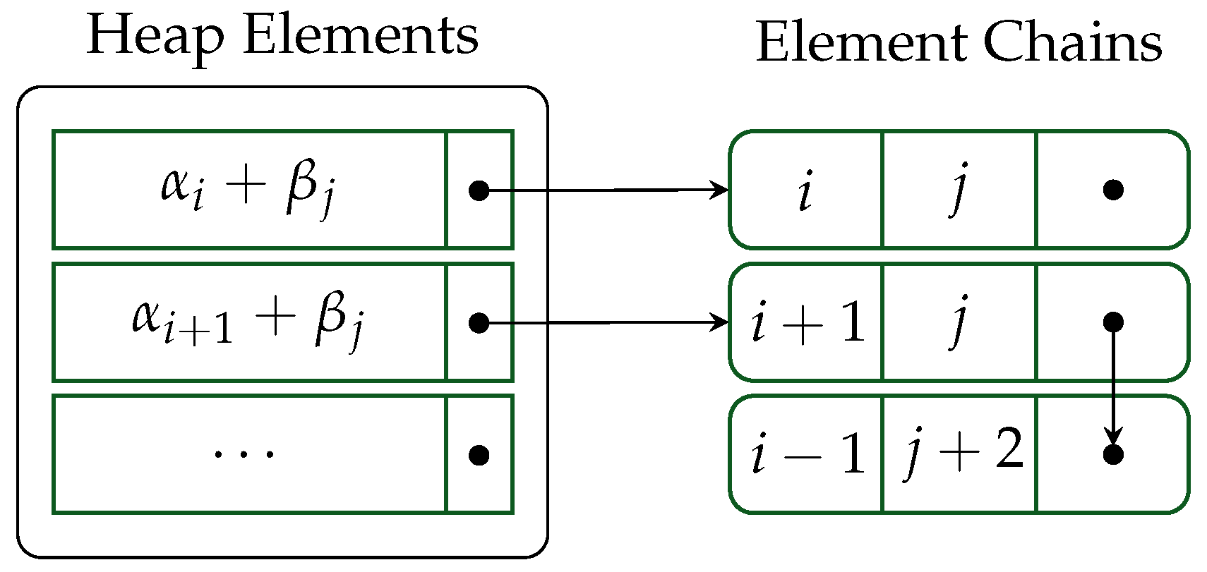
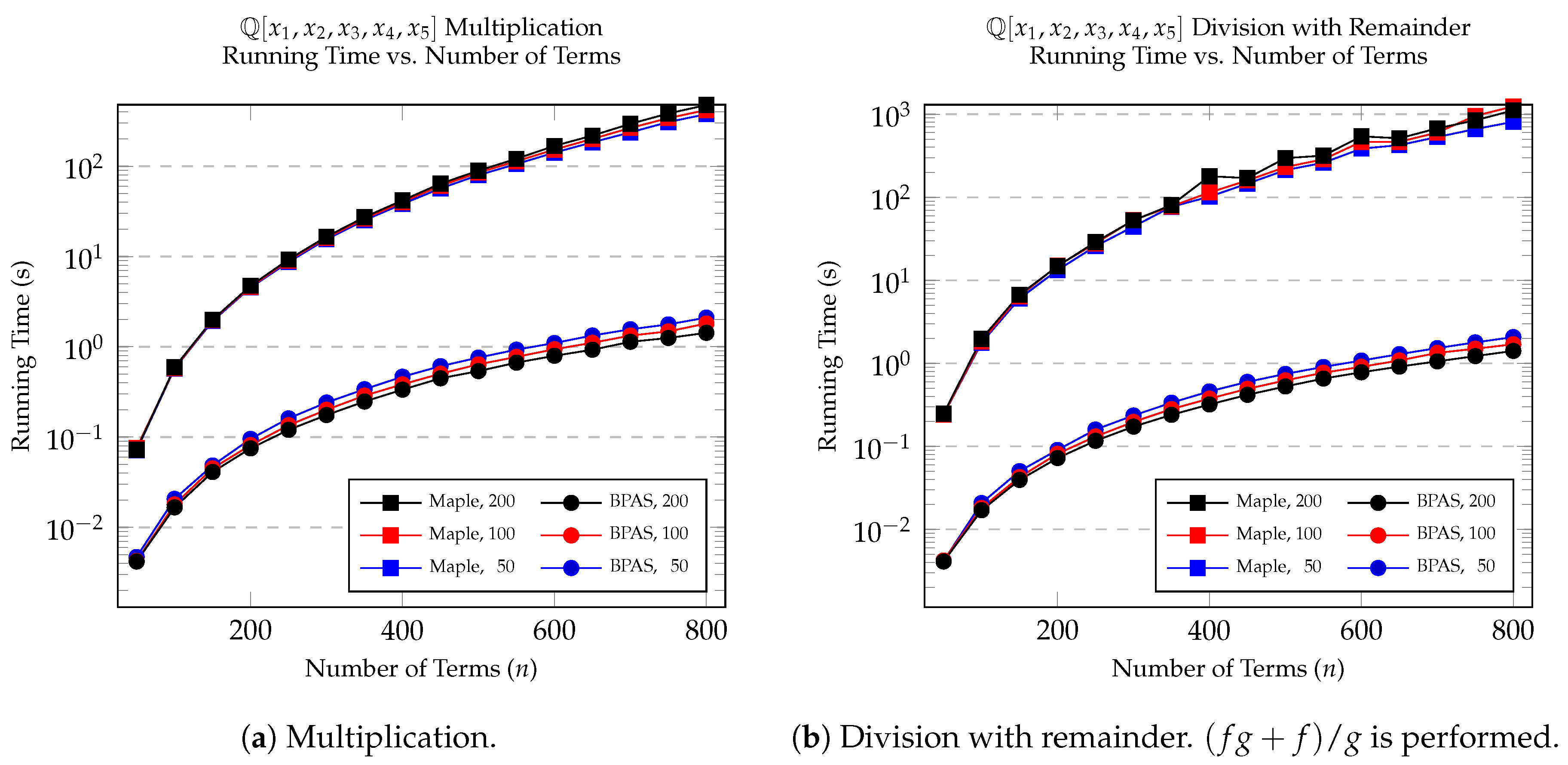
Table 1.
Comparing multiplication and division on the three structured problems.
| Operation | d | Coef. Bound | BPAS | Maple | ||
|---|---|---|---|---|---|---|
| Time (s) | Memory (MiB) | Time (s) | Memory (MiB) | |||
| Multiplication | 4 | 1 | 4.28 | 172.11 | 1.78 | 79.31 |
| 4 | 64 | 8.22 | 353.27 | 9.58 | 810.23 | |
| 5 | 64 | 155.51 | 2481.37 | 221.71 | 5569.25 | |
| Division | 4 | 64 | 7.84 | 353.29 | 6.465 | 816.03 |
| 5 | 64 | 154.08 | 2509.42 | 124.37 | 5583.50 | |
| Multiplication | 12 | 1 | 3.61 | 702.14 | 2.835 | 439.21 |
| 12 | 32 | 7.62 | 1878.96 | 52.80 | 4026.29 | |
| 15 | 32 | 51.61 | 8605.52 | 1114.23 | 18,941.05 | |
| Division | 12 | 32 | 8.09 | 1919.28 | 10.35 | 4033.57 |
| 15 | 32 | 57.09 | 8627.16 | 58.906 | 18,660.94 | |
| Division | 1,000,000 | 1 | 0.18 | 38.59 | 1.505 | 164.54 |
| 10,000,000 | 1 | 1.87 | 522.65 | 23.63 | 1102.21 | |
© 2019 by the authors. Licensee MDPI, Basel, Switzerland. This article is an open access article distributed under the terms and conditions of the Creative Commons Attribution (CC BY) license (http://creativecommons.org/licenses/by/4.0/).
Share and Cite
MDPI and ACS Style
Asadi, M.; Brandt, A.; Moir, R.H.C.; Moreno Maza, M. Algorithms and Data Structures for Sparse Polynomial Arithmetic. Mathematics 2019, 7, 441. https://doi.org/10.3390/math7050441
AMA Style
Asadi M, Brandt A, Moir RHC, Moreno Maza M. Algorithms and Data Structures for Sparse Polynomial Arithmetic. Mathematics. 2019; 7(5):441. https://doi.org/10.3390/math7050441
Chicago/Turabian StyleAsadi, Mohammadali, Alexander Brandt, Robert H. C. Moir, and Marc Moreno Maza. 2019. "Algorithms and Data Structures for Sparse Polynomial Arithmetic" Mathematics 7, no. 5: 441. https://doi.org/10.3390/math7050441
Note that from the first issue of 2016, this journal uses article numbers instead of page numbers. See further details here.