Fractional Calculus as a Simple Tool for Modeling and Analysis of Long Memory Process in Industry


Faculty of BERG, Technical University of Košice, Němcovej 3, 04200 Košice, Slovakia
*
Author to whom correspondence should be addressed.
Mathematics 2019, 7(6), 511; https://doi.org/10.3390/math7060511
Submission received: 25 April 2019
/
Revised: 1 June 2019
/
Accepted: 3 June 2019
/
Published: 4 June 2019
(This article belongs to the Special Issue Fractional Order Systems)
Abstract
:This paper deals with the application of the fractional calculus as a tool for mathematical modeling and analysis of real processes, so called fractional-order processes. It is well-known that most real industrial processes are fractional-order ones. The main purpose of the article is to demonstrate a simple and effective method for the treatment of the output of fractional processes in the form of time series. The proposed method is based on fractional-order differentiation/integration using the Grünwald–Letnikov definition of the fractional-order operators. With this simple approach, we observe important properties in the time series and make decisions in real process control. Finally, an illustrative example for a real data set from a steelmaking process is presented.
1. Introduction
In this paper, we discuss how the fractional calculus is used in modeling and analysis of fractional-order processes (e.g., a real industrial process). Fractional-order processes are characterized by long memory, local memory or heavy-tailed distributions. These properties cannot be neglected in time series analysis. The fractional calculus provides a tool for both long memory and local memory process analysis.
Long memory processes are known to play an important role in many areas of science and technology. The idea of applying a fractional-order model in time series analysis is not new. In the last 20 years, a significant progress has been made in understanding the probabilistic foundations and statistical principles of such processes. For instance, the Hurst exponent was used as a measure of long-term memory of time series [1]. In [2] a fractionally differenced autoregressive-moving average process was used. Nowadays, fractional calculus, fractional-order systems, fractional-order processes and fractional signal processing techniques and their real world applications in various areas have been described in several works [3,4,5,6,7,8]. Long memory has been observed even in economics [9]. A very useful application of the fractional calculus in the time series analysis of heart rate variability was shown in [10]. Some new fractional (a.k.a. fractal) time series models and processes have been discussed in the tutorial review [11].
In this article, we propose a useful tool for applied researchers and practitioners who need to analyze data in which power laws, long memory, self-similar scaling or fractal properties are relevant. We combine the two modeling approaches: statistical analysis and the fractional calculus.
2. Preliminaries
2.1. Fractional Calculus
Fractional calculus has been known since the beginning of integer-order calculus, as it dates back to the 1695 correspondence between Leibniz and L’Hospital. It is a generalization of integration and differentiation to a non-integer order fundamental operator , where a and b are the bounds of the operation and is an arbitrary order. The usual notation for the left-sided fractional-order integro-differential operator of a function defined within the interval is , with . The basic theory was developed mainly in the 19th century, and engineering applications were realized mainly in the second half of the 20th century. There exist a lot of definitions of fractional-order operators (integrals and derivatives) for constant, variable, distributed and even complex order. However, in this paper, we consider only the Grünwald–Letnikov definition of constant order, which is equivalent to other definitions (Caputo, Riemann–Liouville) for a wide class of the functions, under certain conditions [5].
Definition 1.
The Grünwald–Letnikov definition of the fractional-order operator is given as [5]:
where means the integer part.
The form (1) of the fractional operator definition is very helpful for finding a numerical approximation of fractional derivatives/integrals as well as the solution of fractional differential equations. For the definition of binomial coefficients, we may use the relation based on Euler’s Gamma function, defined as follows:
where
2.2. Fractional-Order Processes
It is well-known that a fractional-order process can be considered as the output of a fractional-order system, and has long memory properties. The essence of fractional-order processes is a power-law, which demonstrates the long memory itself. Generally, there is a large number of real processes, where the fractional calculus can be applied [8]. Westerlund proposed a description of a “universal process” by the following equation [13]:
where the input, , is an intensive signal, the output, , is extensive, and parameters, k and , are the process constants. For example, for electrical processes, the electrical current is an extensive signal, and the electrical voltage is an intensive signal. Similarly, for mechanical processes, it is force and position; for heat processes, it is heat flux and temperature, and so on [14]. Thus, the fractional-order processes are widely found in science, technology and engineering systems [6].
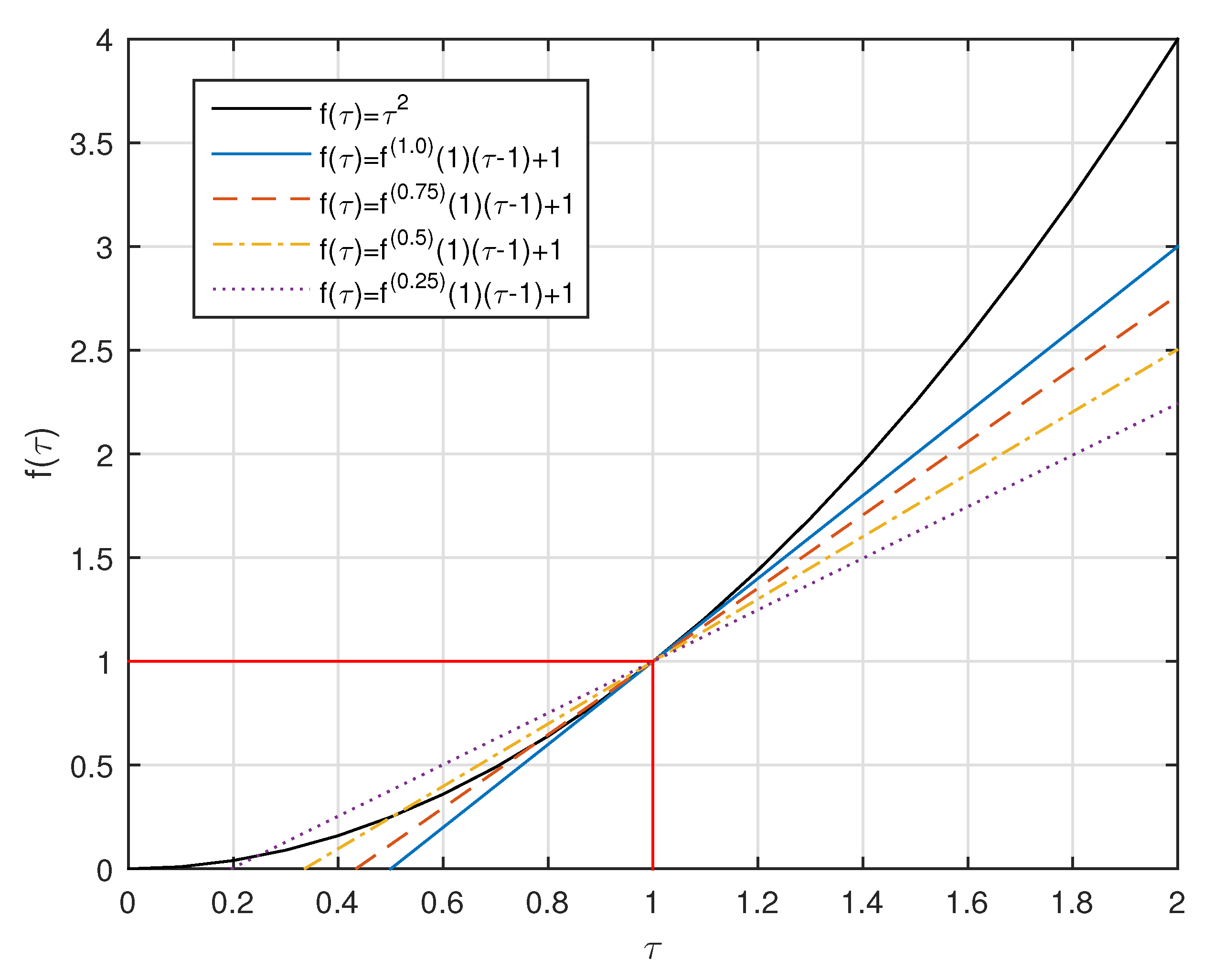
Moreover, the use of fractional-order derivatives for the description and analysis of real processes also requires their geometrical interpretation [3,15,16,17,18]. For example, let us consider the function as an intense signal. The line passing through the point , is given by the equation
where is the slope of the line. Figure 1 shows the plot of a function with lines formed with fractional order derivatives at the point .
In the case of the first-order derivative, the slope of the line is equal to the tangent line. The tangent angle of the line slope at a given point in the function depends on the value of the fractional-order derivative at the considered point.
Definition 2.
According to the Grünwald–Letnikov definition (1), the tangent of the angle θ can be expressed as follows:
or
where binomial coefficients represent the weight of the effect of the function history, respectively, the sum partially accumulate the history of the function. For the binomial coefficients , an expression (8) can be used.
2.3. Fractional Time Series
Fractional time series are characterized by the Hurst exponent (parameter). The Hurst exponent H was originally developed by Harold Edwin Hurst in hydrology for determining optimal dam sizing for the Nile river. It is directly related to fractal dimension D, such that . The Hurst exponent is defined as follows [19,20,21]:
Definition 3.
Let us consider d as a duration, which is a period of time that includes several points in the time series over the range R as a difference between the largest and smallest deviation encountered during a duration d, then we can write:
where H is the Hurst exponent. It means that the higher the Hurst exponent is, the smoother the curve is.
The Hurst exponent is used as a measure of long memory in a time series. It takes on values from 0 to 1. A value of 0.5 indicates the lack of long-range dependence, and the time series has no statistical dependence. Absolute values of the autocorrelation functions decay exponentially to zero. A parameter H less than 0.5 corresponds to anti-persistency. When H exceeds one half and is closer to 1, it indicates greater degree of persistence or long-range dependence. For the cases and , power-law decay is typically observed. Time series that are Gaussian may be analyzed efficiently, but those which exhibit anti-persistence (negatively correlated process) or persistence (positively correlated process) resist simple analysis. By using the operation of fractional integration to an anti-persistent time series (or fractional differentiation to a persistent time series), Gaussian behavior can be observed.
3. Proposed Method and Analysis Tool
As was mentioned in the previous section, there exists a technique for correcting the data to remove the anti-persistence or persistence by applying fractional calculus of order . This yields data that obey Gaussian statistics and therefore the time series can be processed and analyzed. Thus, if a white Gaussian process is fractional differ-integrated with order , then the acquired time series has the Hurst parameter equal to . Fractional integration and differentiation are significant novelties in analysis because of the improved accuracy of estimates and properties of the series. If a series is not described properly, then further analyses will not be accurate. A review of methods for the estimation of the Hurst parameter, which are helpful as simple diagnostic tools for time series, was given in [6]. The R/S method is one of the most well-known estimators. A useful Matlab function for the exponent estimation is available [22].
Moreover, for numerical computation of the fractional-order operation, the following formula derived from the Grünwald–Letnikov definition (1), at the points , can be used [4]:
where , T is the time step of calculation (sampling period) and the binomial coefficients can be calculated according to recurrence relation:
By applying both aforementioned techniques, we obtain a powerful tool for analysis of real (fractional-order) processes, especially in the case, when we do not have enough a priori information about the process due to a lack of measured information, etc.
4. Example: Modeling and Analysis of Industrial Process
4.1. Process Description
In this example, the data of the steelmaking process in a basic oxygen furnace located at U.S. Steel Košice, Ltd., Slovak Republic, are presented. The data of 240 melts were collected during the year 2018. The basic oxygen furnace is a pear shaped vessel, where pig iron from the blast furnace and ferrous scrap is refined into steel by blowing high-purity oxygen through the hot metal. This large vessel has a capacity of up to 400 tons of melt at high temperatures of 1650 to 1700 C. It is a highly complex thermochemical process with high energy consumption. The heat energy is obtained by burning mainly carbon and silicon that are in the inputs. The basic material inputs to the basic oxygen furnace process are pig iron, ferrous scrap, slag additives, and blown oxygen. The outputs of the process consist of steel, slag, and waste gas [24,25].
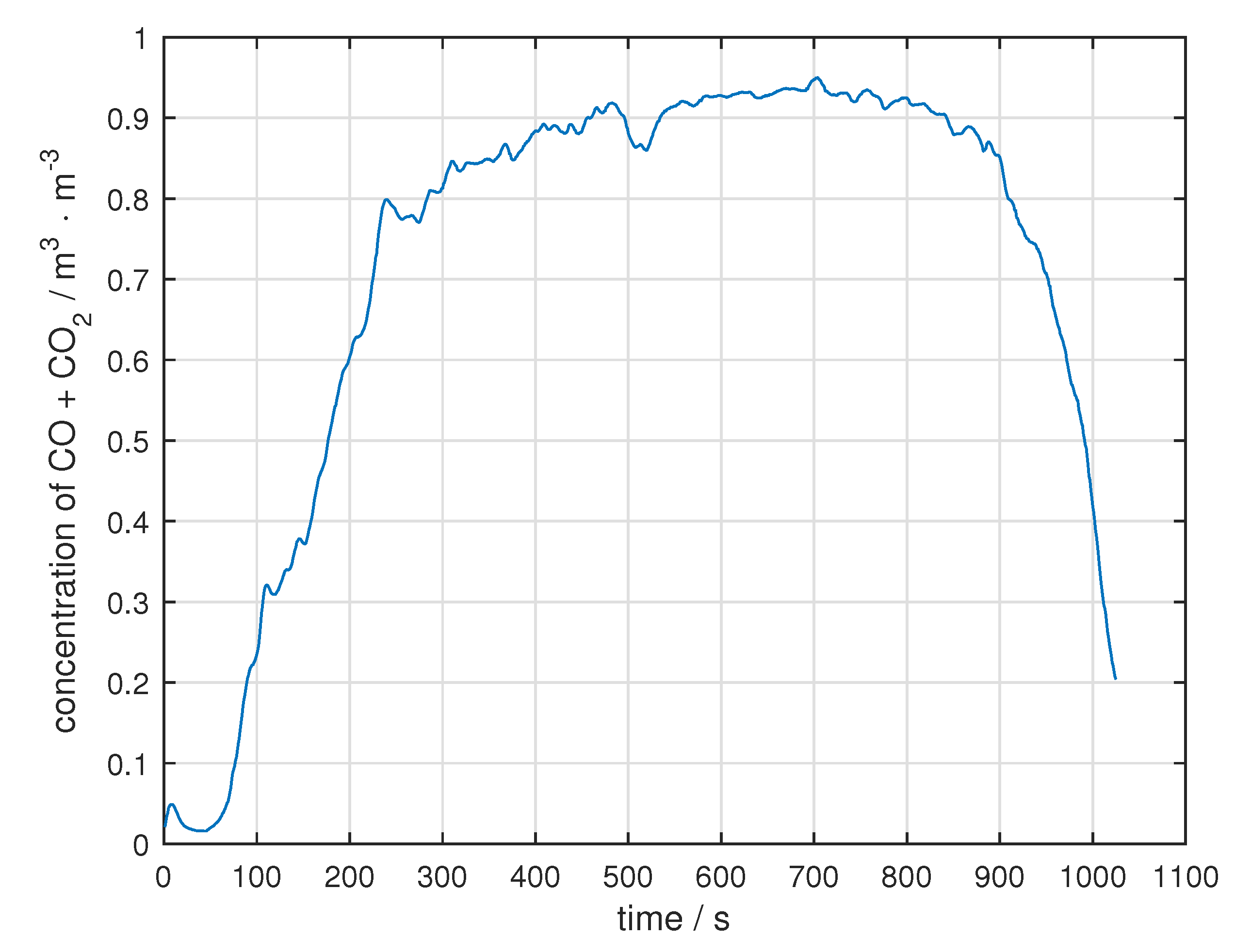
Very important information about the process and at the end of the process is the concentration of carbon monoxide and carbon dioxide in the waste gas (see Figure 2 for one selected melt). At the start of the process, the concentration is zero, and the concentration then increases to maximum values, and at the end decreases to zero again. Similarly, the change of the total concentration of carbon oxides corresponds to the decarburization rate. In terms of process control, the decarburization rate below a certain threshold value means terminating the process in the basic oxygen furnace.
The decarburation rate can be given by
where is the measured waste gas flow, and are measurement concentration of carbon monoxide and carbon dioxide in the waste gases, and is the molar volume [26]. Calculation of the decarburization rate according to Equation (9) is only possible in the case where the waste gas flow is measured. If the waste gas flow is not measured, we need to find a method to determine the end of the process. Taking into account the information about of the fractional-order process, we applied the new proposed method.
4.2. Process Analysis
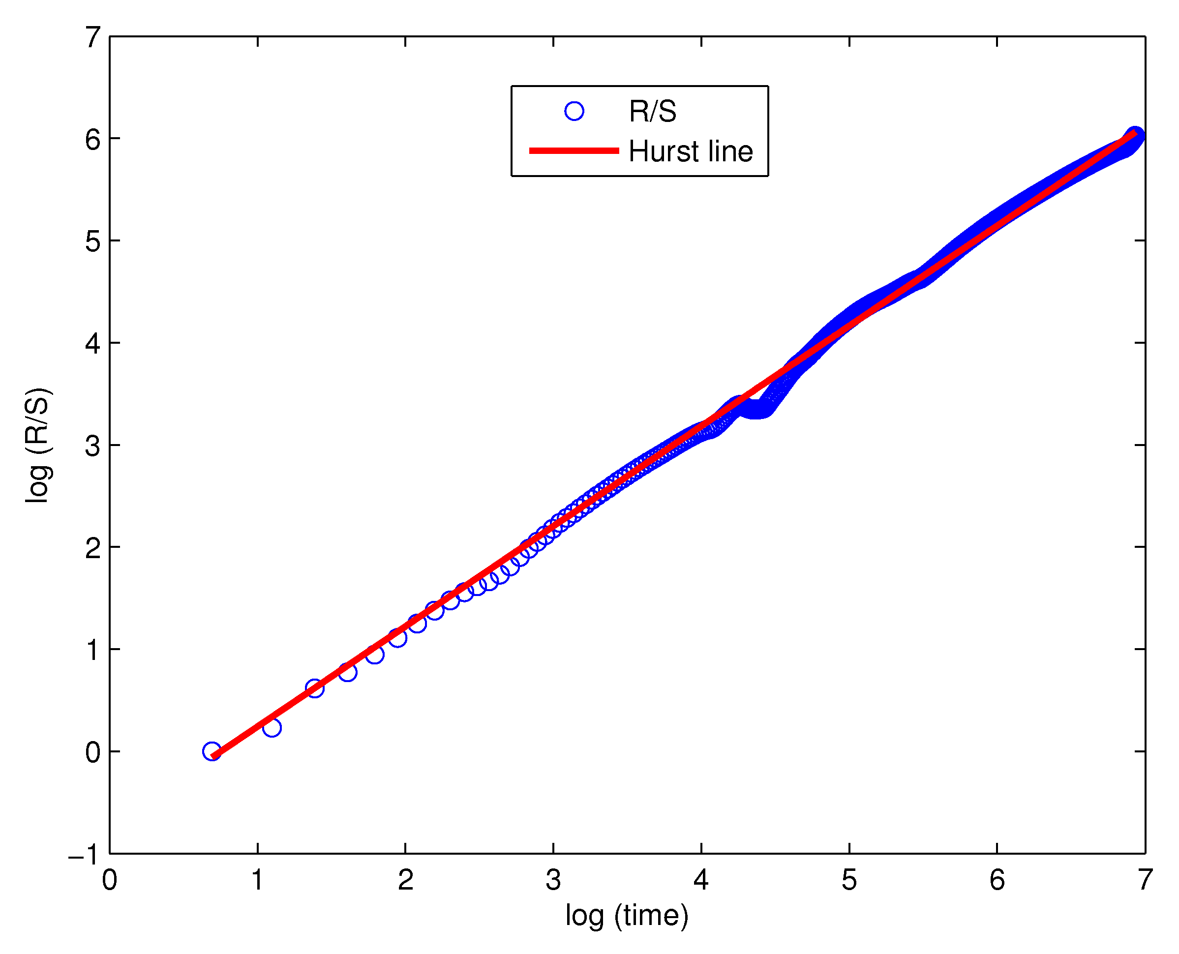
Signal depicted in Figure 2 is a long memory process and a typical long-range dependence time series, with the Hurst exponent , where R/S statistic and Hurst line is depicted as log-log plot in Figure 3. The slope of the line gives the Hurst exponent.
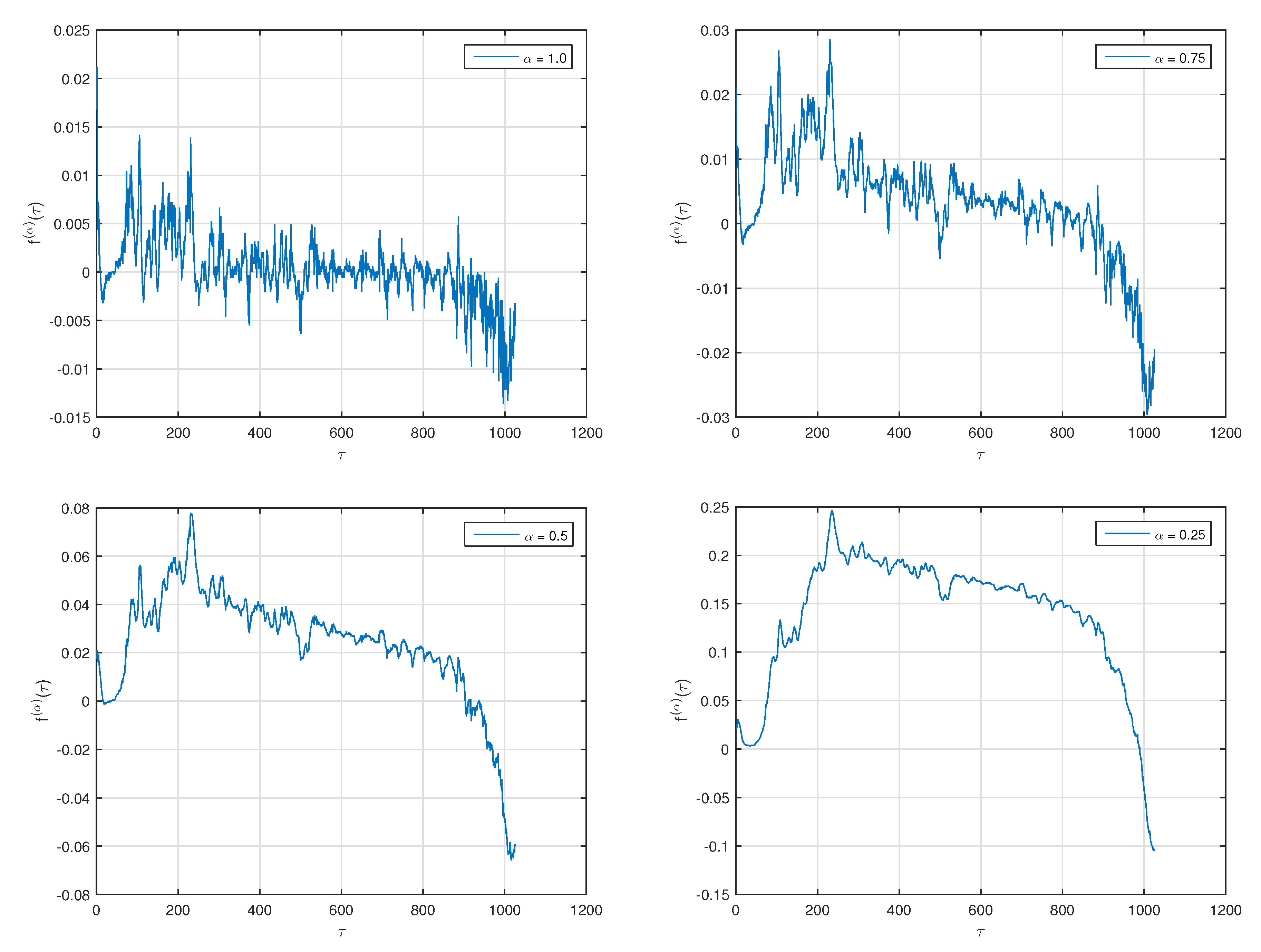
The signals, which exhibit fractional properties, should be investigated using the fractional calculus technique to obtain better analysis results. Using the relation (7) derived from the Grünwald–Letnikov definition (1), for s, the change of the concentration of carbon oxides for various orders is shown in Figure 4. We used the same melt as is depicted in Figure 2. In the case of the first-order derivative, the values move in a narrow range around a value equal to zero, and, at the end of the process, there is a slight decrease. This is because the first-order derivative means roughly the difference of two consecutive values of the function. In the case of the derivative of order less than one, the values move above the zero and only fall below the limit value if the process ends. This follows from the memory effect, that is, that the value of the fractional-order derivative of the function is affected by all previous function values. The question is which order of derivative we should use.
The use of half-order derivatives for the computation of heat flux, based on the known history of temperatures, was described in [5,12]. If we generalize this case, then it is possible to use half-order derivatives for the computation of the extensive signal behavior (heat flow, mass flow, electric current, and so on), based on the known behavior of the intensive signal (temperature, concentration, electrical potential, and so on).
In our case, the mass flow of carbon () is proportional to the concentration of carbon oxides () as
The data analysis of 240 melts was undertaken. Different orders of fractional differentiation within interval the were calculated for all concentrations of the considered melts, as it is depicted in Figure 4. Subsequently, the end point value or minimum value was determined. Table 1 shows and compares the values of the statistical indices for the orders obtained from all 240 melts. Because of different values, a relative standard deviation in percent as a measure of variability was also calculated. The values indicate that the smallest relative standard deviation is between and .
4.3. Simulation Results and Discussion
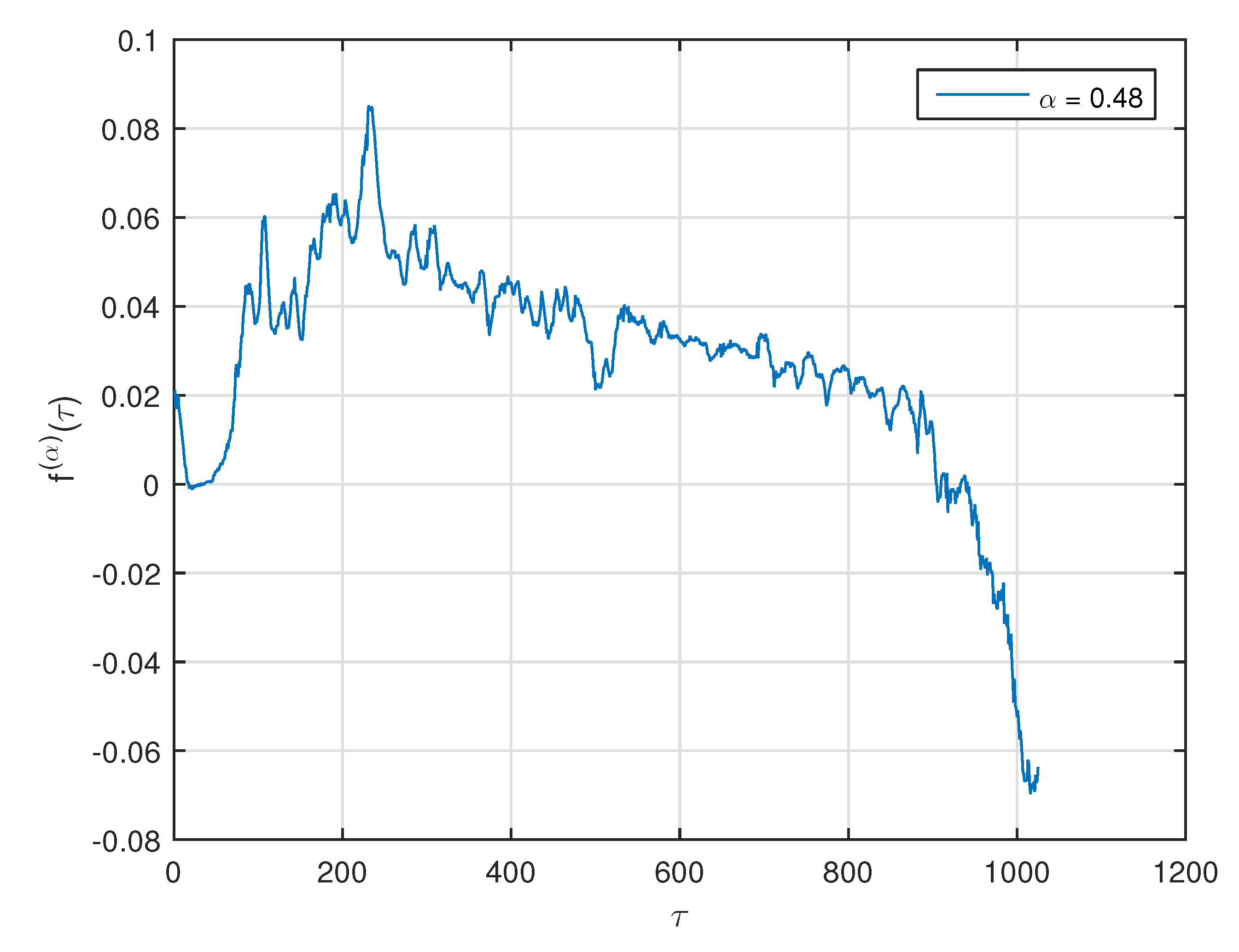
From the above results, it follows that, for the given device, we can determine the process endpoint using the fractional derivative of the concentration of carbon oxides. The value of the derivative order and the endpoint value should be determined for each basic oxygen furnace separately based on the analysis of the measured data during long period. It should be noted that, according to the fractional time series theory, the order of fractional derivative should correspond to the Hurst exponent of measured data in the time series. It is an effective tool that is useable for various long memory processes. For the melt depicted in Figure 2, the Hurst exponent was obtained. For accurate determination of the end point in the process, we should analyze the fractionally differentiated time series with order , which also corresponds to the results obtained by statistical analysis shown in Table 1.
In Figure 5, the change of CO and CO concentration for order for one particular melt is depicted as it was shown in Figure 2. From the figure, we may determine the process end point which is extremely significant for the furnace operator. In the presented case, the process end point is approximately at 900 s. Since the steelmaking process is a process characterized by high energy consumption, the accurate finishing time of each melt is very important for minimizing production costs.
Moreover, the order of differentiation applied to the time series (measured data) moderates the curve shape (function) as it was demonstrated in Figure 1, as well as by the relations (5) or (6), where the history of the function is considered. In the case of a basic oxygen furnace, the function is the concentration of carbon oxides.
5. Conclusions
In this paper, we described a simple tool for the modeling and analysis of long memory processes such as the steelmaking process. This approach is based on the Grünwald–Letnikov definition of fractional-order operator (derivative/integral). In this particular case, we used this definition because of data being presented in a time series, where the other definitions are not appropriate for such data processing since the data are given as a sequence, not a function. Obviously, for mathematical modeling where the process can be described by a function, it is more suitable to use Caputo’s definition mainly because of better setting of initial conditions. However, another advantage for using the Grünwald–Letnikov definition is the possibility of using a short memory principle [5], especially in industry, where the hardware devices have limited memory and processor speed.
Combining two known mathematical tools, the fractional calculus technique and statistical methods, we obtain a simple but powerful tool to determine the process end point from measured data in the form of time series without direct measurement of the necessary exact value, in our case, the waste gas flow measurement. It is extremely important for industry to minimize costs as well as technical difficulties with making such a measurement.
We presented the techniques and tools for data processing with references for Matlab functions. Finally, an illustrative example of a real industrial process is given to demonstrate the effectiveness of obtained results.
Author Contributions
This work involved all coauthors. I.P. wrote the original draft and contributed to the software and the editing. J.T. analyzed the data, contributed to the visualization and investigated the results.
Funding
This research was funded by the Slovak Research and Development Agency under the contract No. APVV-14-0892, No. SK-AT-2017-0015, and by the Slovak Grant Agency for Science under Grant No. VEGA 1/0365/19 and No. VEGA 1/0273/17.
Conflicts of Interest
The authors declare no conflict of interest.
References
- Diebolt, C.; Guiraud, V. Long Memory Time Series and Fractional Integration. A Cliometric Contribution to French and German Economic and Social History. Hist. Soc. Res. 2000, 25, 4–22. [Google Scholar]
- Li, W.K.; McLeod, A.I. Fractional time series modelling. Biometrika 1986, 73, 217–221. [Google Scholar] [CrossRef]
- Bandyopadhyay, B.; Kamal, S. Stabilization and Control of Fractional Order Systems; Springer: Cham, Switzerland, 2015. [Google Scholar]
- Petráš, I. Fractional-Order Nonlinear Systems: Modeling, Analysis and Simulation; Springer: New York, NY, USA, 2011. [Google Scholar]
- Podlubny, I. Fractional Differential Equations; Academic Press: San Diego, CA, USA, 1999. [Google Scholar]
- Sheng, H.; Chen, Y.Q.; Qiu, T.S. Fractional Processes and Fractional-Order Signal Processing; Springer: London, UK, 2012. [Google Scholar]
- Sun, H.G.; Zhang, Y.; Baleanu, D.; Chen, W.; Chen, Y.Q. A new collection of real world applications of fractional calculus in science and engineering. Commun. Nonlinear Sci. Numer. Simulat. 2018, 64, 213–231. [Google Scholar] [CrossRef]
- West, B.J. Fractional Calculus View of Complexity; CRC Press: New York, NY, USA, 2016. [Google Scholar]
- Tarasov, V.E.; Tarasova, V.V. Dynamic Keynesian Model of Economic Growth with Memory and Lag. Mathematics 2019, 7, 178. [Google Scholar] [CrossRef]
- Garcia-Gonzalez, M.A.; Fernandez-Chimeno, M.; Capdevila, L.; Parrado, E.; Ramos-Castro, J. An application of fractional differintegration to heart rate variability time series. Comput. Methods Programs Biomed. 2013, 111, 33–40. [Google Scholar] [CrossRef] [PubMed]
- Li, M. Fractal Time Series—A Tutorial Review. Math. Probl. Eng. 2010, 2010, 157264. [Google Scholar] [CrossRef]
- Oldham, K.B.; Spanier, J. The Fractional Calculus; Academic Press: New York, NY, USA, 1974. [Google Scholar]
- Westerlund, S. Dead Matter Has Memory! Causal Consulting: Kalmar, Sweden, 2002. [Google Scholar]
- Doebelin, E.O. System Dynamics: Modeling and Response; Merrill: Columbus, OH, USA, 1972. [Google Scholar]
- Podlubny, I. Geometric and physical interpretation of fractional integration and fractional differentiation. Fract. Calc. Appl. Anal. 2002, 4, 357–366. [Google Scholar]
- Nizami, S.T.; Khan, N.; Khan, F.H. A new approach to represent the geometric and physical interpretation of fractional order derivatives of polynomial function and its application in field of science. Can. J. Comput. Math. Nat. Sci. Eng. Med. 2010, 1, 1–8. [Google Scholar]
- Machado, J.A.T. A probabilistic interpretation of the fractional-order differentiation. Fract. Calc. Appl. Anal. 2003, 1, 73–80. [Google Scholar]
- Moshrefi-Torbati, M.; Hammond, J.K. Physical and geometrical interpretation of fractional operators. J. Frankl. Inst. 1998, 6, 1077–1086. [Google Scholar] [CrossRef]
- Oldham, K.B. An introduction to the fractional calculus and some applications. In Proceedings of the Second International Workshop—Transform Methods and Special Functions, Varna, Bulgaria, 23–30 August 1996; pp. 598–609. [Google Scholar]
- Liu, K.; Chen, Y.Q.; Zhang, X. An Evaluation of ARFIMA (Autoregressive Fractional Integral Moving Average) Programs. Axioms 2017, 6, 16. [Google Scholar] [CrossRef]
- Pavlíčková, M.; Petráš, I. A note on time series data analysis using a fractional calculus technique. In Proceedings of the 15th International Carpathian Control Conference (ICCC), Velke Karlovice, Czech Republic, 28–30 May 2014; pp. 424–427. [Google Scholar]
- Abramov, V. Hurst Exponent Estimation; Matlab Central File Exchange; MathWorks, Inc.: Natick, MA, USA, 2018; Available online: https://www.mathworks.com/matlabcentral/fileexchange/39069 (accessed on 23 April 2019).
- Petráš, I. Digital Fractional Order Differentiator/Integrator—FIR Type; Matlab Central File Exchange; MathWorks, Inc.: Natick, MA, USA, 2003; Available online: http://www.mathworks.com/matlabcentral/fileexchange/3673 (accessed on 23 April 2019).
- Oeters, F. Metallurgy of Steelmaking; Verlag Stahleisen mbH: Düsseldorf, Germany, 1994. [Google Scholar]
- Turkdogan, E.T. Fundamentals of Steelmaking; Maney Publishing: Leeds, UK, 2010. [Google Scholar]
- Kattenbelt, C.; Roffel, B. Dynamic Modeling of the Main Blow in Basic Oxygen Steelmaking Using Measured Step Responses. Met. Mater. Trans. B 2008, 5, 764–769. [Google Scholar] [CrossRef]
Figure 1.
Plot of the function with lines formed with fractional-order derivatives at the point .

Figure 2.
The change of CO and CO concentration.

Figure 3.
The slope of the Hurst line.

Figure 4.
The change of CO and CO concentration for various orders .

Figure 5.
The change of CO and CO concentration for order .


Table 1.
Statistical values for the process end point.
| Arithmetic Mean | Median | Range R | Standard Deviation S | Relative Standard Deviation | |
|---|---|---|---|---|---|
| 0.0 | 0.001552 | 0.001157 | 0.008391 | 0.001753 | 112.99 |
| 0.1 | −0.110144 | −0.110675 | 0.058425 | 0.012487 | 11.33 |
| 0.2 | −0.135971 | −0.135620 | 0.072973 | 0.013492 | 9.92 |
| 0.3 | −0.124915 | −0.125612 | 0.050907 | 0.010584 | 8.47 |
| 0.4 | −0.102376 | −0.101533 | 0.035958 | 0.007871 | 7.68 |
| 0.5 | −0.079537 | −0.078806 | 0.026901 | 0.006659 | 8.37 |
| 0.6 | −0.060418 | −0.060031 | 0.030330 | 0.006287 | 10.40 |
| 0.7 | −0.046102 | −0.044751 | 0.032936 | 0.006192 | 13.43 |
| 0.8 | −0.035730 | −0.034599 | 0.037782 | 0.006508 | 18.21 |
| 0.9 | −0.028537 | −0.027227 | 0.042185 | 0.006910 | 24.21 |
| 1.0 | −0.023569 | −0.021991 | 0.044271 | 0.007089 | 30.07 |
© 2019 by the authors. Licensee MDPI, Basel, Switzerland. This article is an open access article distributed under the terms and conditions of the Creative Commons Attribution (CC BY) license (http://creativecommons.org/licenses/by/4.0/).
Share and Cite
MDPI and ACS Style
Petráš, I.; Terpák, J. Fractional Calculus as a Simple Tool for Modeling and Analysis of Long Memory Process in Industry. Mathematics 2019, 7, 511. https://doi.org/10.3390/math7060511
AMA Style
Petráš I, Terpák J. Fractional Calculus as a Simple Tool for Modeling and Analysis of Long Memory Process in Industry. Mathematics. 2019; 7(6):511. https://doi.org/10.3390/math7060511
Chicago/Turabian StylePetráš, Ivo, and Ján Terpák. 2019. "Fractional Calculus as a Simple Tool for Modeling and Analysis of Long Memory Process in Industry" Mathematics 7, no. 6: 511. https://doi.org/10.3390/math7060511
Note that from the first issue of 2016, this journal uses article numbers instead of page numbers. See further details here.