Non-Intrusive Inference Reduced Order Model for Fluids Using Deep Multistep Neural Network

Abstract
1. Introduction
1.1. Related Work
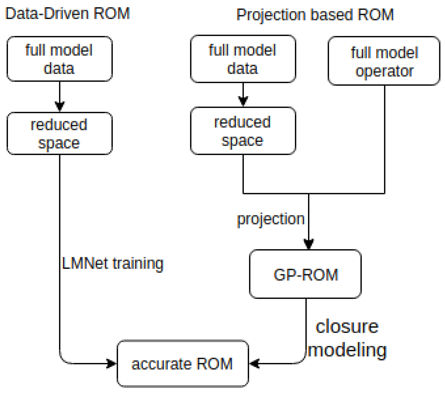
1.2. Our Approach
- A novel non-intrusive learning reduced order model framework for fluid dynamics, which is applicable to general nonlinear dynamical systems with sophisticated legacy codes.
- Our framework overcomes the instability issue of the projection based model reduction, and provides accurate approximation and long-term prediction of the full system.
- The learning process of our approach is more computationally efficient than the construction of reduced operators in the classic projection based methods.
2. Reduced Order Modeling
3. Learning Reduced Order Model
3.1. Rom Dynamics
3.2. Linear Multistep Network (LMNet)
3.3. LMNet-ROM
| Algorithm 1 Linear multistep network reduced order model learning (LMNet-ROM). |
| Compute the reduced POD space from the data of NSE by (3) Compute the training dataset B via (12) Train the neural network using loss function (14) The LMNet-ROM for NSE is obatined from the trained low-dimensional dynamic system: |
4. Numerical Experiment
4.1. Implementation Details
4.2. Full Order Model Approximation
4.3. Long-Term Prediction
4.4. LMNet-ROM vs. Closure Models
4.5. Computational Cost
5. Conclusions and Outlook
Author Contributions
Funding
Acknowledgments
Conflicts of Interest
Abbreviations
| FOM | Full order model |
| ROM | Reduced order model |
| LMNet | Linear multistep neural network |
| POD | Proper orthogonal decomposition |
| CFD | Computational fluid dynamics |
| DNS | Direct numerical simulation |
| GP-ROM | Galerkin projection reduced-order model |
| EF-ROM | Evolve-then-filter reduced-order model |
| DDF-ROM | Data-driven filtered reduced-order model |
| NSE | Naiver–Stokes equations |
| AM | Adams–Moulton |
Appendix A. Loss Function
References
- Lumley, J.L. The structure of inhomogeneous turbulent flows. Atmos. Turbul. Radio Wave Propag. 1967, 2, 166–178. [Google Scholar]
- Noack, B.R.; Morzynski, M.; Tadmor, G. Reduced-Order Modelling for Flow Control; Springer: Berlin/Heidelberg, Germany, 2011; Volume 528. [Google Scholar]
- Obinata, G.; Anderson, B.D. Model Reduction for Control System Design; Springer Science & Business Media: Berlin/Heidelberg, Germany, 2012. [Google Scholar]
- Carlberg, K.; Farhat, C.; Cortial, J.; Amsallem, D. The GNAT method for nonlinear model reduction: Effective implementation and application to computational fluid dynamics and turbulent flows. J. Comput. Phys. 2013, 242, 623–647. [Google Scholar] [CrossRef]
- Rowley, C.W.; Dawson, S.T. Model reduction for flow analysis and control. Ann. Rev. Fluid Mech. 2017, 49, 387–417. [Google Scholar] [CrossRef]
- Amsallem, D.; Farhat, C. Stabilization of projection-based reduced-order models. Int. J. Numer. Meth. Eng. 2012, 91, 358–377. [Google Scholar] [CrossRef]
- Xie, X.; Wells, D.; Wang, Z.; Iliescu, T. Approximate deconvolution reduced order modeling. Comput. Methods Appl. Mech. Eng. 2017, 313, 512–534. [Google Scholar] [CrossRef]
- Kutz, J.N.; Brunton, S.L.; Brunton, B.W.; Proctor, J.L. Dynamic Mode Decomposition: Data-Driven Modeling of Complex Systems; SIAM: Philadelphia, PA, USA, 2016; Volume 149. [Google Scholar]
- San, O.; Maulik, R. Extreme learning machine for reduced order modeling of turbulent geophysical flows. Phys. Rev. E 2018, 97, 042322. [Google Scholar] [CrossRef] [PubMed]
- Xiao, D.; Fang, F.; Buchan, A.; Pain, C.; Navon, I.; Muggeridge, A. Non-intrusive reduced order modelling of the Navier–Stokes equations. Comput. Methods Appl. Mech. Eng. 2015, 293, 522–541. [Google Scholar] [CrossRef]
- Peherstorfer, B.; Willcox, K. Data-driven operator inference for nonintrusive projection-based model reduction. Comput. Methods Appl. Mech. Eng. 2016, 306, 196–215. [Google Scholar] [CrossRef]
- Noack, B.R.; Stankiewicz, W.; Morzyński, M.; Schmid, P.J. Recursive dynamic mode decomposition of transient and post-transient wake flows. J. Fluid Mech. 2016, 809, 843–872. [Google Scholar] [CrossRef]
- Loiseau, J.C.; Brunton, S.L. Constrained sparse Galerkin regression. J. Fluid Mech. 2018, 838, 42–67. [Google Scholar] [CrossRef]
- Carlberg, K.; Barone, M.; Antil, H. Galerkin v. discrete-optimal projection in nonlinear model reduction. arXiv 2015, arXiv:1504.03749. [Google Scholar]
- Balajewicz, M.J.; Dowell, E.H.; Noack, B.R. Low-dimensional modelling of high-Reynolds-number shear flows incorporating constraints from the Navier–Stokes equation. J. Fluid Mech. 2013, 729, 285–308. [Google Scholar] [CrossRef]
- Ballarin, F.; Manzoni, A.; Quarteroni, A.; Rozza, G. Supremizer stabilization of POD–Galerkin approximation of parametrized steady incompressible Navier–Stokes equations. Int. J. Numer. Meth. Engng. 2015, 102, 1136–1161. [Google Scholar] [CrossRef]
- Xie, X.; Mohebujjaman, M.; Rebholz, L.; Iliescu, T. Data-driven filtered reduced order modeling of fluid flows. SIAM J. Sci. Comput. 2018, 40, B834–B857. [Google Scholar] [CrossRef]
- Protas, B.; Noack, B.R.; Östh, J. Optimal nonlinear eddy viscosity in Galerkin models of turbulent flows. J. Fluid Mech. 2015, 766, 337–367. [Google Scholar] [CrossRef]
- Ostrowski, Z.; Białecki, R.; Kassab, A. Solving inverse heat conduction problems using trained POD-RBF network inverse method. Inverse Probl. Sci. Eng. 2008, 16, 39–54. [Google Scholar] [CrossRef]
- Rogers, C.A.; Kassab, A.J.; Divo, E.A.; Ostrowski, Z.; Bialecki, R.A. An inverse POD-RBF network approach to parameter estimation in mechanics. Inverse Probl. Sci. Eng. 2012, 20, 749–767. [Google Scholar] [CrossRef]
- Xiao, D.; Fang, F.; Pain, C.; Hu, G. Non-intrusive reduced-order modelling of the Navier–Stokes equations based on RBF interpolation. Int. J. Numer. Methods Fluids 2015, 79, 580–595. [Google Scholar] [CrossRef]
- San, O.; Maulik, R. Neural network closures for nonlinear model order reduction. Adv. Comput. Math. 2018, 44, 1717–1750. [Google Scholar] [CrossRef]
- Chang, B.; Meng, L.; Haber, E.; Tung, F.; Begert, D. Multi-level residual networks from dynamical systems view. arXiv 2017, arXiv:1710.10348. [Google Scholar]
- Lu, Y.; Zhong, A.; Li, Q.; Dong, B. Beyond finite layer neural networks: Bridging deep architectures and numerical differential equations. arXiv 2017, arXiv:1710.10121. [Google Scholar]
- Brunton, S.L.; Proctor, J.L.; Kutz, J.N. Discovering governing equations from data by sparse identification of nonlinear dynamical systems. Proc. Natl. Acad. Sci. USA 2016, 113, 3932–3937. [Google Scholar] [CrossRef]
- Rudy, S.H.; Brunton, S.L.; Proctor, J.L.; Kutz, J.N. Data-driven discovery of partial differential equations. Sci. Adv. 2017, 3, e1602614. [Google Scholar] [CrossRef]
- Raissi, M.; Karniadakis, G.E. Hidden physics models: Machine learning of nonlinear partial differential equations. J. Comput. Phys. 2018, 357, 125–141. [Google Scholar] [CrossRef]
- Raissi, M.; Perdikaris, P.; Karniadakis, G.E. Machine learning of linear differential equations using Gaussian processes. J. Comput. Phys. 2017, 348, 683–693. [Google Scholar] [CrossRef]
- Wang, Z.; Xiao, D.; Fang, F.; Govindan, R.; Pain, C.C.; Guo, Y. Model identification of reduced order fluid dynamics systems using deep learning. Int. J. Numer. Methods Fluids 2018, 86, 255–268. [Google Scholar] [CrossRef]
- Chen, T.Q.; Rubanova, Y.; Bettencourt, J.; Duvenaud, D. Neural Ordinary Differential Equations. arXiv 2018, arXiv:1806.07366. [Google Scholar]
- Parish, E.J.; Duraisamy, K. A paradigm for data-driven predictive modeling using field inversion and machine learning. J. Comput. Phys. 2016, 305, 758–774. [Google Scholar] [CrossRef]
- Gouasmi, A.; Parish, E.J.; Duraisamy, K. A priori estimation of memory effects in reduced-order models of nonlinear systems using the Mori–Zwanzig formalism. Proc. R. Soc. A 2017, 473, 20170385. [Google Scholar] [CrossRef] [PubMed]
- Wells, D.; Wang, Z.; Xie, X.; Iliescu, T. An evolve-then-filter regularized reduced order model for convection-dominated flows. Int. J. Numer. Methods Fluids 2017, 84, 598–615. [Google Scholar] [CrossRef]
- Raissi, M.; Perdikaris, P.; Karniadakis, G.E. Multistep Neural Networks for Data-driven Discovery of Nonlinear Dynamical Systems. arXiv 2018, arXiv:1801.01236. [Google Scholar]
- Ascher, U.M.; Petzold, L.R. Computer Methods for Ordinary Differential Equations and Differential-Algebraic Equations; SIAM: Philadelphia, PA, USA, 1998; Volume 61. [Google Scholar]
- Embree, M. Numerical Analysis Lecture Notes. February 2018. Available online: http://www.math.vt.edu/people/embree/math5466/nanotes.pdf (accessed on 15 June 2019).
- Zhang, X.; Li, Z.; Change Loy, C.; Lin, D. Polynet: A pursuit of structural diversity in very deep networks. In Proceedings of the IEEE Conference on Computer Vision and Pattern Recognition, Honolulu, HI, USA, 21–26 July 2017; pp. 718–726. [Google Scholar]
- Schäefer, M.; Turek, S. The benchmark problem “flow around a cylinder”. Flow Simul. High-Perform. Comput. II 1996, 52, 547566. [Google Scholar]
- Brunton, S.; Tu, J.; Bright, I.; Kutz, J. Compressive sensing and low-rank libraries for classification of bifurcation regimes in nonlinear dynamical systems. SIAM J. Appl. Dyn. Syst. 2014, 13, 1716–1732. [Google Scholar] [CrossRef]
- Mohebujjaman, M.; Rebholz, L.G.; Xie, X.; Iliescu, T. Energy balance and mass conservation in reduced order models of fluid flows. J. Comput. Phys. 2017, 346, 262–277. [Google Scholar] [CrossRef]
- Caiazzo, A.; Iliescu, T.; John, V.; Schyschlowa, S. A numerical investigation of velocity-pressure reduced order models for incompressible flows. J. Comput. Phys. 2014, 259, 598–616. [Google Scholar] [CrossRef]


| Neurons | 64 | 128 | 256 | |
|---|---|---|---|---|
| Layers | ||||
| 1 | ||||
| 2 | ||||
| 3 | ||||
| Dimension | r = 4 | r = 6 | r = 8 | |
|---|---|---|---|---|
| K/model | ||||
| 1 | ||||
| 2 | ||||
| 3 | ||||
| 4 | ||||
| GP-ROM | ||||
| Model | GP-ROM | LMNet-ROM | |
|---|---|---|---|
| Noise | |||
| 0.0% | |||
| 0.5% | |||
| 1% | |||
| 5% | |||
| Dimension | r = 4 | r = 6 | r = 8 | |
|---|---|---|---|---|
| Model | ||||
| EF-ROM | ||||
| DDF-ROM | ||||
| LMNet-ROM | ||||
| Model | Cost | Speed-Up Factor () |
|---|---|---|
| GP-ROM | 855.52 s | 43.05 |
| EF-ROM | 867.20 s | 42.47 |
| DDF-ROM | 6373.97 s | 5.78 |
| LMNet-ROM | 445.25 s | 82.71 |
© 2019 by the authors. Licensee MDPI, Basel, Switzerland. This article is an open access article distributed under the terms and conditions of the Creative Commons Attribution (CC BY) license (http://creativecommons.org/licenses/by/4.0/).
Share and Cite
Xie, X.; Zhang, G.; Webster, C.G. Non-Intrusive Inference Reduced Order Model for Fluids Using Deep Multistep Neural Network. Mathematics 2019, 7, 757. https://doi.org/10.3390/math7080757
Xie X, Zhang G, Webster CG. Non-Intrusive Inference Reduced Order Model for Fluids Using Deep Multistep Neural Network. Mathematics. 2019; 7(8):757. https://doi.org/10.3390/math7080757
Chicago/Turabian StyleXie, Xuping, Guannan Zhang, and Clayton G. Webster. 2019. "Non-Intrusive Inference Reduced Order Model for Fluids Using Deep Multistep Neural Network" Mathematics 7, no. 8: 757. https://doi.org/10.3390/math7080757
APA StyleXie, X., Zhang, G., & Webster, C. G. (2019). Non-Intrusive Inference Reduced Order Model for Fluids Using Deep Multistep Neural Network. Mathematics, 7(8), 757. https://doi.org/10.3390/math7080757