PM2.5 Prediction Model Based on Combinational Hammerstein Recurrent Neural Networks


1
Department of Industrial Engineering and Management, National Yunlin University of Science and Technology, College of Management, Main Campus, Yunlin 64002, Taiwan
2
Feng-Chia University, Taichung 40724, Taiwan
*
Author to whom correspondence should be addressed.
Mathematics 2020, 8(12), 2178; https://doi.org/10.3390/math8122178
Submission received: 7 November 2020
/
Revised: 3 December 2020
/
Accepted: 4 December 2020
/
Published: 6 December 2020
(This article belongs to the Special Issue Applied Data Analytics)
Abstract
:Airborne particulate matter 2.5 (PM2.5) can have a profound effect on the health of the population. Many researchers have been reporting highly accurate numerical predictions based on raw PM2.5 data imported directly into deep learning models; however, there is still considerable room for improvement in terms of implementation costs due to heavy computational overhead. From the perspective of environmental science, PM2.5 values in a given location can be attributed to local sources as well as external sources. Local sources tend to have a dramatic short-term impact on PM2.5 values, whereas external sources tend to have more subtle but longer-lasting effects. In the presence of PM2.5 from both sources at the same time, this combination of effects can undermine the predictive accuracy of the model. This paper presents a novel combinational Hammerstein recurrent neural network (CHRNN) to enhance predictive accuracy and overcome the heavy computational and monetary burden imposed by deep learning models. The CHRNN comprises a based-neural network tasked with learning gradual (long-term) fluctuations in conjunction with add-on neural networks to deal with dramatic (short-term) fluctuations. The CHRNN can be coupled with a random forest model to determine the degree to which short-term effects influence long-term outcomes. We also developed novel feature selection and normalization methods to enhance prediction accuracy. Using real-world measurement data of air quality and PM2.5 datasets from Taiwan, the precision of the proposed system in the numerical prediction of PM2.5 levels was comparable to that of state-of-the-art deep learning models, such as deep recurrent neural networks and long short-term memory, despite far lower implementation costs and computational overhead.
1. Introduction
Airborne particulate matter (PM) can have a profound effect on the health of the population. This type of pollution is generally divided into PM2.5 and PM10, based on the diameter of the particles, where PM2.5 indicates a maximum size of 2.5 μm and PM10 indicates a maximum size of 10 μm. PM2.5 tends to remain in the atmosphere for much longer, it tends to be carried far greater distances, and is small enough to penetrate deep within tissue, often leading to serious respiratory disorders. It is for this reason that most research on particulate matter pollution focuses on PM2.5–related issues. There has also been considerable effort in developing methods by which to predict PM2.5 levels in order to prepare the public. Most existing systems rely on extensive monitoring in conjunction with statistical analysis or artificial intelligence technology to perform time-series forecasting [1]. In statistical analysis, Baur et al. [2] employed conditional quantile regression to simulate the influences of meteorological variables on ozone concentration in Athens. Sayegh et al. [3] utilized multiple statistical models, including a multiple linear regression model, a quantile regression model, a generalized additive model, and boosted regression Trees1-way and 2-way to predict PM10 concentrations in Mecca. More recently, Delavar et al. [4] examined the effectiveness of using geographically weighted regression to predict two different series of data: PM10 and PM2.5 in Tehran. In artificial intelligence, Sun et al. [5] applied a hidden Markov model to predict 24-h-average PM2.5 concentrations in Northern California. Delavar et al. [4] used a support vector machine to predict the PM10 and PM2.5 concentrations in Tehran. Various shallow neural networks have also been used to analyze and predict air pollution values. For instance, Biancofiore et al. [6] employed a recursive neural network to predict PM2.5 concentrations on the Adriatic coast. Zhang and Ding [7] used an extreme learning machine to predict air pollution values in Hong Kong. Yang and Zhou [8] recently merged autoregressive moving average models with the wavelet transform to predict the values. Ibrir et al. [9] used a modified support vector machine to predict the values of PM1, PM2.5, PM4, and PM10. Shafii et al. [10] used a support vector machine to predict PM2.5 values in Malaysia. Hu et al. [11] used the random forest algorithm to make numerical predictions of PM2.5 values. Lagesse et al. [12] and Wang et al. [13] used shallow neural networks to predict PM2.5 values. Liu and Chen [14] designed a three-stage hybrid neural network model to enhance the accuracy of PM2.5 predictions. Despite claims pertaining to the efficacy of these methods, there is compelling evidence that they are not as effective at dealing with PM2.5 as for other pollutants. PM2.5 can be attributed to local or external sources. Local sources can be direct emissions or the irregular products of photochemical effects in the atmosphere, which can cause drastic fluctuations in PM2.5 concentrations within a short period of time. In contrast, it is also important to consider external sources. That is, PM2.5 is extremely light and can be easily transported by the monsoon, which creates by the long-term but periodic pollution. The fact that PM2.5 concentrations present gradual fluctuations over the long term, as well as radical changes over the short term, makes it very difficult to make predictions using many methods based on statistics or artificial intelligence.
Numerous researchers have demonstrated the efficacy of deep learning models in formulating predictions [15,16,17]. Freeman et al. [15] used deep learning models to predict air quality. Huang and Kuo [16] designed the convolutional neural network-long short-term memory deep learning model to predict PM2.5 concentrations. Tao et al. [17] merged the concept of 1-dimension conversion with a bidirectional gated recurrent unit in developing a deep learning model aimed at enhancing the accuracy of air pollution forecasts. Pak et al. [18] recently used a deep learning model to assess spatiotemporal correlations to predict air pollution levels in Beijing. Liu et al. [19] used attention-based long short-term memory and ensemble-learning to predict air pollution levels. Ding et al. [20] developed the correlation filtered spatial-temporal long short-term memory model to predict PM 2.5 concentrations. Ma et al. [21] designed a Bayesian-optimization-based lag layer long short-term memory fully connected network to obtain multi-sequential-variant PM2.5 predictions. Li et al. [22] used an ensemble-based deep learning model to estimate PM2.5 concentrations over California. Zheng et al. [23] used micro-satellite images, convolutional neural networks, and a random forest approach to estimate PM2.5 values at the surface. Overall, deep learning models have proven highly in predicting PM2.5 concentrations.
In practice, the implementation of deep learning models imposes a heavy burden [24,25,26] in constructing the model and obtaining real-time predictions for hundreds of locations every day. Below, we present an example case illustrating the implementation of a deep learning model to predict costs associated with PM2.5 prediction. In this case, the national meteorological bureau is tasked with obtaining forecasts at 500 locations throughout the country. Without loss of generality, we can assume that formulating PM2.5 predictions involves combining five separate long short-term memory (LSTM) outcomes. To maintain prediction accuracy, the agency must retrain all of the LSTMs at intervals of five days based on the most recent data. The meteorological bureau has four deployment options. Table 1 lists the monetary costs (in 2020 prices) and time costs of the options as follows: (1) Ordinary computer with one central processing unit (CPU) only and no graphics processing unit (GPU) (USD 1000; 10,000 s to train each LSTM), such that 289 days would be required to complete a round of LSTM training at all 500 sites. (2) Mid-range computer with three GPUs (USD 17,000; 11 days required to complete a round of LSTM training at 500 sites (assuming 400 s per iteration). Despite the relatively low hardware cost, the computation time is excessive. (3) Four mid-range computers as above (USD 68,000; 3 days to complete a round of LSTM training at 500 sites. (4) Supercomputer (USD 10,000,000; 0.1 s to train each LSTM, such that 250 s would be required to complete a round of LSTM training). Scenarios (3) and (4) meet the requirements of the meteorological bureau; however, the costs are very high. Note also that the above-mentioned costs are only for a single pollutant. Most monitoring systems must deal with 20 to 30 pollutants as well as conventional forecasting of weather patterns and typhoons. Clearly, the use of deep learning models for the prediction of pollutants and weather systems is far beyond the financial means of many countries, such as Guinea [27] and Bangladesh [28]. A new approach to computation is required.
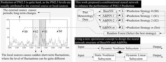
Accordingly, this study proposed a combinational Hammerstein recurrent neural network (CHRNN) to overcome these limitations. The operational concept of the proposed model is shown in Figure 1. The inputs of the CHRNN include recent meteorological data from a weather observation station, and the output is the predicted value of PM2.5 for a future time point. The CHRNN contains a based-neural network (based-NN) and several add-on neural networks (AddNNs). The former is used to learn long-term changes in PM2.5 data, and the latter is used to learn sudden changes in PM2.5 data. Low-level learning is used for the more common sudden changes, and high-level learning is used for sparsely sudden changes. Considering superimposing the results of the AddNNs layer-by-layer onto the prediction results of the based-NN, the CHRNN can then produce multiple prediction strategies. As shown in Figure 1, the prediction result of strategy 0 is the output of the based-NN, and the prediction result of strategy 1 is the combined output of the based-NN and AddNN-1. In addition, the CHRNN also includes a random forest that determines the output strategies of the CHRNN based on historical meteorological data, where Figure 2 can be illustrated as an example. Suppose the PM2.5 value follows usual periodic changes such as those in Section A. Then, the random forest will determine that only strategy 0 is needed for predictions. In contrast, if the PM2.5 values show unusual changes of varying magnitudes, such as shown in Sections B and C, then the random forest will recommend that strategy 1 and strategy 2, respectively, be used to obtain better prediction results. For the framework of the based-NN and AddNNs, we employed the well-known Hammerstein recurrent neural network (HRNN) [29] into our model. This framework splits a dynamic nonlinear time series data into a static nonlinear module and a dynamic linear module for modeling, respectively, which is shown in Figure 3. This way, the dynamic behavior in the time series will only be processed by the dynamic linear module, where the nonlinear behavior will only be processed by the static nonlinear module. Therefore, it enhanced the modeling of prediction accuracy [29,30]. Furthermore, the CHRNN is modeled based on shallow neural networks, the construction and operation costs of which are far lower than those of deep learning models. In the following, we use the example in Table 1 to emphasize the merits of employing CHRNN in deep learning models. Assume that the meteorological bureau needs to train 2500 CHRNNs (500 locations × 5 CHRNNs per location) every five days. By only using an ordinary computer (one CPU and no GPUs), the construction of each CHRNN could be completed within 100 s. This means only approximately 25,000 s (3 days) would be required to complete a round of training. This is a considerable improvement over the 289 days and USD 68,000 that would be required under the previous scenario.
We anticipate that the CHRNN will improve the accuracy and lower the costs of PM2.5 predictions. However, we encountered two difficulties: (1) The first difficulty includes the selection of features to predict PM2.5 values, which may also have a time-delay terms problem. That is, how far into the past, should we go to collect the data for applying these features? This has been considered by many researchers and consequently has been the focus of a wide variety of discussions. Past approaches can be roughly divided into two categories: (i) based on professional knowledge regarding air pollution, several meteorological items are chosen as features [2,4,31], or (ii) correlations between all data items, and the output is first examined before the most relevant items are chosen as features [6,15,17]. Note that the former may result in the selection of unsuitable features, thereby producing poor prediction accuracy. However, while the latter may lead to the selection of more suitable features, the issue of time-delay terms is seldom taken into account, which also affects prediction accuracy. This study developed the modified false nearest neighbor method (MFNNM) to overcome it. (2) The second difficulty we encountered is to determine a means of enabling the based-NN to learn the periodic long-term changes in PM2.5 concentrations and the AddNNs to learn the sudden short-term variations in PM2.5 concentrations. We developed the usual case emphasizing normalization (UCENormalization) method to address this issue. Finally, we conducted simulations using real-world datasets of a one-year period from Taichung, Taiwan. These experiments verified that the proposed approach might achieve greater prediction accuracy than deep learning models at lower costs.
The proposed method provides predictive accuracy superior to that of existing machine-learning methods for a given construction cost. In other words, the proposed method makes it possible to achieve the accuracy of advanced deep learning models without having to invest any more than would be required to establish a machine learning system.
2. Related Works
This chapter outlines previous numerical methods for forecasting air pollution using machine learning technology and introduces related research on Hammerstein recurrent neural networks.
2.1. Existing Machine Learning Methods for the Prediction of Air Pollution
Numerical forecasting methods can be broadly divided according to whether they are based on atmospheric sciences, statistical methods, or machine learning [24]. In the past, most prediction schemes have used statistical analysis or methods developed in the atmospheric sciences; however, machine learning has moved to the forefront, particularly in forecasting air pollution, due to the heavy reliance of atmospheric sciences on domain expertise and extensive data sets [32,33]. Statistical methods are easily applied to the numerical forecasting of air pollution [2,3,34,35,36] without the need for arcane professional knowledge; however, this approach is highly constrained by the nature of the data, which means that they are inapplicable to situations that have yet to occur. The complexity of fluctuations in air pollution levels cannot be adequately dealt with using historical data. Thus, there remains considerable room for improvement in real-world PM2.5 predictions.
Machine learning has become a mainstream method for forecasting air pollution levels. This approach does not require extensive domain knowledge, and predictions can be formulated under a wide range of parameters, often exceeding those found in existing datasets. Sun et al. [5] used a hidden Markov model to predict air pollution values. Delavar et al. [4] performed similar predictions using a support vector machine. Hu et al. [11], Huang et al. [37], Liu et al. [38], and Stafoggia et al. [39] used the random forest algorithm to make numerical predictions of PM2.5 concentrations. Many researchers have begun using shallow neural networks or deep learning models for the prediction of air pollution values. Lagesse et al. [12] used a shallow neural network to predict indoor PM2.5 values. Wang et al. [13] used a basic neural network to predict air pollution in Chongqing, China. Liu and Chen [14] designed a three-stage hybrid neural network model to facilitate the numerical prediction of outdoor PM2.5 levels. Pak et al. [18] used spatiotemporal correlations in conjunction with a deep learning model to predict air pollution values in Beijing. Liu et al. [19] employed attention-based long short-term memory and ensemble-learning to predict air pollution concentrations. Zheng et al. [23] used micro-satellite images in conjunction with a convolutional neural network and random forest approach to estimate PM2.5 values on the surface. Chen and Li [24] recently designed a radial basis function—long short-term memory to identify key meteorological observations in neighboring stations to assist in predicting PM2.5 values. Note that those key observations can also be used to improve the accuracy of other machine learning models. Overall, machine-learning methods are the preferred approach by which to formulate predictions pertaining to air pollution.
2.2. Hammerstein Recurrent Neural Network
The Hammerstein recurrent neural network is currently one of the most effective shallow neural networks for time-series prediction [29,40]. Time-series prediction has always been regarded as a difficult problem due to the nonlinear dynamic characteristics of complex systems. Essentially, the time value of t + 1 is affected by the previous time values of t, t − 1, …, t − n (dynamic system), and there is a nonlinear relationship between the first few time values and the value of t + 1. Hammerstein subsystem models [41,42,43] are meant to overcome this problem. They comprise a static nonlinear subsystem with a dynamic linear system operating in series, as shown in Figure 3. This provides two benefits when modeling and predicting time series: (1) The dynamic behavior of the time series is processed by a dynamic linear module, whereas the nonlinear behavior is processed by a static nonlinear module. This greatly facilitates modeling and improves accuracy. (2) Numerous mathematical models, such as a nonlinear regression model or neural network, can be used to replace the static nonlinear subsystem and dynamic linear system, thereby making it possible to customize time-series prediction problems. The Hammerstein subsystem model has been widely used in a variety of fields. Westwick and Kearney [41] and Dempsey and Westwick [42] applied a Hammerstein subsystem model to model the dynamic stretch reflex system. Abd-Elrady and Gan [43] achieved good results by applying a Hammerstein subsystem model to signal processing. Mete et al. [44] employed a similar approach in system identification.
Since confirming the efficacy of this approach in modeling the effects of dynamic nonlinear systems, scholars have been combining Hammerstein subsystem models with neural networks. Wang and Chen [45] implemented a Hammerstein subsystem model in conjunction with a recursive fuzzy neural network to deal with time-series prediction and signal noise elimination. Wang and Chen [29] integrated a recurrent neural network within a Hammerstein subsystem model to overcome various automatic control problems. Lee et al. [30] recently combined a Hammerstein recurrent neural network with a genetic algorithm to formulate time series of traffic flow on highways. The models mentioned above have clearly demonstrated the effectiveness of combining the Hammerstein subsystem model with a neural network to deal with dynamic nonlinear systems, such as signal processing, control problems, or time series prediction.
3. Study Area, Dataset and Data Preprocessing
The meteorological data collected in this study comprised hourly data collected in 2018 by three air-quality monitoring stations run by the Environmental Protection Administration (DaLi, FengYuan, and ChungMing) in Taichung, Taiwan. The locations of the monitoring stations are shown in Figure 4. We considered these three stations because they are situated in areas where air pollution is the most severe and the population is the densest. From each station, we collected 12 types of data associated with air pollution, including levels of PM2.5, PM10, CO, O3, SO2, NO, and NO2, wind speed, hourly wind speed, relative humidity, temperature, and rainfall. Note that although general meteorological observatories provide air quality index (AQI) values, we opted not to consider AQI values in the current paper. AQI values are derived from particulate matter concentrations as well as carbon monoxide, sulfur dioxide, and nitrogen dioxide, and tropospheric ozone levels. From a mathematical perspective, AQI values are highly dependent on at least one of the above values. Thus, even if we input AQI in addition to the five above-mentioned values, the corresponding improvement in prediction accuracy would be negligible due to overlap. Furthermore, entering AQI values would greatly increase computational overhead by increasing the dimensionality of the data. Of course, it would be possible to formulate predictions based solely on AQI values; however, this would not adequately reflect the variations in the five pollution values. The exclusive use of AQI values for prediction would reduce the scope of the five pollution values, leading to a corresponding decrease in prediction accuracy.
These datasets contained many missing values or errors, and the errors may have continued for varying amounts of time. We employed the linear interpolation method used [15] to replace the missing values or correct the abnormalities. The interpolation method depended on how long the missing values or errors continued. If they continued for less than 24 h, we used the values of the time periods before and after the period in question for interpolation. This way, the calibration results would best correspond to the conditions of that day. In addition, if the values that needed to be replaced covered more than 24 h, then we used the average supplementing value of the 24 h periods before and after the period in question for interpolation. With such a large range of missing values or errors, it may produce difficulty for us to recover the conditions on the day in question. Therefore, we could only use the conditions of the previous and subsequent days to simulate the possible air quality conditions during the same time of the day.
Figure 5 displays the PM2.5-time series results after data cleaning, and Table 2 presents the value distributions in the datasets. As shown in Table 2, the PM2.5 values at each location can fluctuate drastically within a two-hour period, at the most exceeding half the range of the dataset. Furthermore, the mean + 3× standard deviation of the three datasets is around 60 ppm, which means that 95% of the data points in these datasets are lower than 60 ppm, and only about 5% of the data are over 60 ppm. Such widely fluctuating and unbalanced data makes predictions using conventional recursive neural networks difficult to model. Hence, a new approach is needed.
4. Research Methods
The PM2.5 prediction process designed in this study includes several parts. It is shown in Figure 6, including (1) using modified false nearest neighbor method (MFNNM) to identify suitable predictive features in the datasets and their time-delay terms; (2) using the usual case emphasizing normalization (UCENormalization) to normalize the PM2.5 time series values to help the based-NN learn the long-term changes in PM2.5 concentrations; (3) constructing the based-NN; (4) constructing several AddNNs based on the modeling results of the based-NN; and (5) constructing a random forest to recommend CHRNN usage strategies for different time points. The details of these five parts are as follows:
4.1. Modified False Nearest Neighbour Method (MFNNM)
The MFNNM can extract suitable predictive features from air-quality data and the corresponding time-delay terms for each feature. The method is grounded on the concepts of the false nearest neighbor method [46,47], which can determine the optimal time-delay terms for features when the features are fixed. However, it cannot be used to select suitable predictive features. Therefore, we modified this method to meet the needs of this study. We first develop the mathematical model of the system under analysis, then introduce the operational concept of MFNNM based on said system, and finally discuss each step of MFNNM.
For each multiple-input single-output (MISO) time series modeling problem, suppose we have already collected a set of input features u1(•), u2(•), …, up(•) and the corresponding output value y(•). Then, we can express the prediction system as
where p denotes the number of features, and m is the optimal value of time-delay terms for all features used for prediction. Below, we discuss three concepts underpinning the MFNNM. The first two originate from the theory of the false nearest neighbor method [46,47], while the third is our extended concept. To facilitate our explanation, let the input vector of system f(•) at time t in Equation (1) be X(t) and the predicted value be y(t + 1). (1) If the changes in y(i) consist of all the factors in X(i) at any time point i and X(j) and X(k) at time points j and k have a short Euclidean distance between them, then the values of y(j) and y(k) must also be close to each other. Hereafter, we refer to X(t) as the optimal input vector of the system. (2) If input vector X’(t) is missing some key factors comparing to X(t), then the values of y(j) and y(k) may not be close to each other even if X’(j) and X’(k) at time points j and k have a short Euclidean distance between them. In this case, a false nearest neighbor (FNN) appears, and the MFNNM can continuously add new factors to X’(t) to reduce the appearances of FNNs. Once the factors in the new X’(j) highly overlap those in X(j), the appearances of FNNs will drop drastically close to 0. (3) If input vector X″(t) has more key factors than X(t), then the values of y(j) and y(k) may not be close to each other even if X″(j) and X″(k) at time points j and k have a short Euclidean distance between them. In this case, an FNN appears, and the MFNNM can continuously eliminate factors within X″(t) to reduce the appearance of FNNs. When factors that are less correlated with the output are eliminated, the appearance of FNNs will drop even more drastically. We can then estimate the importance of each factor to the prediction system based on the changes in FNN appearance after each factor is eliminated. The MFNNM uses these three concepts to select a suitable input vector to prevent FNN appearance.
The MFNNM follows two phases. The first phase follows the suggestions of [46,47] and, based on concepts (1) and (2), involves gradually increasing the time-delay terms of a fixed number of features to increase the number of factors in the input vector and obtain the optimal time-delay terms. The second phase is based on the concept (3) and, with the optimal time-delay terms known, involves eliminating different features to reduce the number of factors in the input vector to understand the correlation between each feature and the output. Finally, the most suitable features for predictions are selected based on their correlation with the output. The steps of the MFNNM are described in detail in the following:
Step 1: Collect the system input and output values of the prediction model at k time points: the output is y(t + i) and the input vector is Xm(t + i), m denotes the delay times of the features, and 1 ≤ I ≤ k.
Step 2: Under the settings m = 1 and I = 1, find a time point j with a minimum Euclidean distance between Xm(t + i) and Xm(t + j). Next, check whether an FNN appears using Equation (2):
where R is a threshold value given by the user. If Equation (2) is not supported, then an FNN appears.
Step 3: Add 1 to i and repeat Step 2 until I = k. Then, calculate Perfnn, which is the probability of an FNN appearing at the k time points with the current m.
Step 4: Repeat Steps 2 and 3, adding 1 to m each time to record the Perfnn. When m finally reaches the set value given by the user, the minimum Perfnn is picked among all m values is the optimal time-delay mfinal, and the corresponding Perfnn is named Perfnn_final.
Having found the optimal time-delay terms of the features, we next explain the approach to seeking the optimal predictive features. First, the input vectors are defined under mfinal as Xmfinal(t + i). Next, we check the impact of each feature on the number of FNNs, beginning with the input factor u1 all the way to input factor up, ultimately determining the importance of each feature.
Step 5: From the original input vector Xmfinal(t + i), eliminate the factor of feature l, and the new vector becomes Xmfinal-l(t + i). Next, repeat the process from Step 2 to Step 4 and calculate Perfnn-l.
Step 6: Repeat Step 5. It is decided to add 1 to l each time and recording the corresponding Perfnn-l until l = p. The features are ultimately ranked in ascending order based on the results of |Perfnn_final–Perfnn-l|. The smaller the difference, the more correlation the feature is to the output, and the more it should be considered during modeling. Next, users can choose the features that will be used in the subsequent steps based on the conditions they have set, such as a required number of features or a required degree of feature impact.
4.2. Usual Case Emphasizing Normalization Method
The UCENormalization uses normalization to enhance the learning effectiveness of the based-NN, considering the long-term changes in a PM2.5 time series while reducing the impact of abnormal values on based-NN modeling. The fundamental concept is that the normal conditions in a PM2.5 time series are normalized to cover a wider range in [−1, 1], while the abnormal conditions occupy a smaller range. This way, the based-NN can more easily find the optimal solution for normal conditions, and prediction accuracy is increased. The remaining abnormal conditions are left for the AddNNs to learn. Then, Figure 7 is an example to explain the concept. Figure 7a displays the original PM2.5 time series, except for A, B, C, and D, which indicate sudden circumstances in the PM2.5 values, the values all present relatively normal conditions. Figure 7b displays the results of proportionally normalizing Figure 7a, and Figure 7c presents the results of UCENormalization. A comparison of the two figures shows that most of the normal conditions are compressed to [−1, −0.3) in Figure 7b, while they are compressed to [−1, 0.9) in Figure 7c. Generally speaking, compression of the normal conditions to a smaller range means that the neural network output will also have a smaller range. In addition, the operational range of the weights will also be reduced, which makes it hard for the neural network to find the optimal solution for each weight and final outputs. As shown in Figure 8, the x-axis represents the operational range of each weight in the based-NN, and the y axis indicates the based-NN output corresponding to said weight. Clearly, the compression of the normal conditions to [−1, 0.3) in Figure 7b means that the operational range of the weights will also be constricted (Figure 8a). In contrast, the normalization of the normal conditions to [−1, 0.9) in Figure 7c means that the operational range of the weights in the based-NN is expanded (Figure 8b), which will increase the accuracy of based-NN predictions for normal conditions.
Based on the definitions of normal and abnormal conditions in half-normal distributions, the abnormal threshold values of PM2.5 are set as mean + n standard deviations, where n is adjusted to normal conditions. The normalization formulas for normal and abnormal conditions are shown in Equations (3) and (4):
where u(•) is the PM2.5 time series value; Norm_u(•) is the normalized PM2.5 time series value; n represents the abnormal threshold value set by the user, and m is the upper bound of normalized values for normal conditions. Note that the value distribution ranges of normal conditions and sudden circumstances in the original data should be taken into consideration when m is set. If the value distribution range of sudden circumstances is small, then it is recommended that m be near 0.9 to increase the accuracy of model learning for normal data. If the value distribution range of sudden circumstances is large, however, then it is recommended that m be around 0.7 to prevent the values from being overly compressed, which would affect model learning of sudden values. In the end, the results of any PM2.5 time series normalized using Equations (3) and (4) should fall within the range of [−1, 1].
4.3. Construction of Based-NN
For the framework of the based-NN in the CHRNN, we adopted the HRNN [29,40], the effectiveness of which has already been demonstrated. As shown in Figure 9, it contains a total of four layers: the input layer, the hidden layer, the dynamic layer, and the output layer. The only function of neurons in the input layer is to pass on the input data to the hidden layer. Suppose n features are extracted using MFNNM, and the value of time-delay terms of each feature is m. Thus, the based-NN has (n + 1) × m inputs, where 1 represents a historical PM2.5 value. Next, the hidden layer is linked to establish the static nonlinear module. The neurons in this layer do not use any recursive items, which means they are static, and the nonlinear tangent sigmoid function serves as the nonlinear function. Then, the dynamic layer and the output layer are responsible for establishing the dynamic linear module. The recursive items of the dynamic layer are responsible for handling the dynamic part, while the linear function of the output layer is responsible for the linear part. The output of the based-NN is the normalized PM2.5 value of the next time point. The mathematical framework of the model is presented in Equations (5)–(7). Among those equations, Equation (5) is the formula from the input layer to the hidden layer, Equation (6) is the formula for the dynamic layer, and Equation (7) is the formula for the output layer. Furthermore, in the neurons in layer j, we use Ii(j)(k) and oi(j)(k) to represent the input and output of neuron i at time k.
In the formulas above, w is the weight between the input layer and the hidden layer. The d is the bias value; the a indicates the regression weight of the dynamic layer; the b is the weight between the dynamic layer and the hidden layer, and the c is the weight between the dynamic layer and the output layer.
In the based-NN, we recommend that the number of neurons in the hidden layer and the dynamic layer should be set as the mfinal value calculated using MFNNM. Researchers have demonstrated that setting this value as the number of hidden layers produces optimal modeling results [48]. The back-propagation algorithm is used to train the HRNN. However, due to the limitation of the paper, please refer to [29] for further details.
4.4. Construction of AddNNs
The construction process of the AddNNs is, as shown in Figure 10. The first step is to calculate the “Base_Error”, which is the error between the based-NN prediction results and the actual PM2.5 values. The second step is to use the Base_Error to train AddNN-1, which also uses HRNN for its framework, but the inputs and output are different. Besides the original inputs of the based-NN, the inputs of AddNN-1 also include the Base_Error values of the past m time points. The outputs of AddNN-1 are the normalized results of the Base_Error for the next time point. After completing the training of AddNN-1, the program calculate the Add_1_Error, the error between the Base_Error and the AddNN-1 output. Note that we recommend setting the numbers of neurons in the hidden layer and dynamic layer of the AddNNs to the same as the number of input dimensions. This is because the ideal output of the AddNNs is the error, which may only be related to some particular inputs. If each neuron in the hidden layer can independently process the changes in an input neuron, prediction accuracy is enhanced.
The third step is roughly the same as the second step: (1) construct AddNN-k (the AddNN on layer k based on HRNN), (2) set the inputs and outputs of AddNN-k and train them together, and (3) calculate Add_k_Error (the error between Add_k-1_Error and AddNN-k). This process continues until the number of AddNNs reaches the preset upper bound or until the error reduction in the AddNN on each layer becomes limited.
Finally, when all of the AddNNs have been constructed, the study is designed to produce the various strategy results of the CHRNN. Each strategy result is the sum of the outputs of the based-NN and multiple AddNNs, as shown in Figure 10. For instance, the result of Strategy 0 equals the result of the based-NN alone, the result of Strategy 1 is the sum of the outputs of the based-NN and AddNN-1, and so on.
4.5. Construction of Random Forest to Determine CHRNN Usage Strategies
This section explains how a random forest is constructed to determine the usage strategies of the CHRNN. However, the random forest algorithm is not the focus of this study, so we introduce only the inputs and output of the random forest. For details on the algorithm, please refer to Breiman [48].
The inputs of the random forest in this paper are identical to those of the based-NN. The reason for this was that these features are identified by the MFNNM as the most correlated with future PM2.5 values and are thus helpful for random forest modeling. The output labels of the random forest represent the optimal strategies of the CHRNN at each time point. The study did not use the smallest error between all of the strategies and the actual values as the output label. We designed a new calculation method. Since the output values of different strategies are often close, using the smallest error among the strategies as the output label would result in relatively small differences among strategy outputs, but the conditions of the output labels at each time point would vary, making random forest training procedure become more difficult.
A buffer variable is generated to overcome this problem. The variable increases the chance that Strategy 0 will be determined as the output label, with Strategy 1, the next most likely, and so on. The reason for this design was that Strategy 0 is used to learn normal conditions and should rationally be the most common. The strategies following Strategy 1 are used to predict abnormal conditions that are less common and should be increasingly less likely to be used, so the probability of them becoming output labels is reduced. We introduce how the output labels are calculated, with Θ denoting the buffer variable. Suppose we want to identify the output label at time i, and the CHRNN has γ AddNNs. Thus, there are γ+1 possible output results for the random forest:
- Case 1
- If |Output of Strategy 0-actual value|÷Θ < |Output of Strategy i-actual value|, where 1 ≤ I ≤ γ, then the output label is set as Strategy 0.
- Case 2
- If Case 1 does not hold, and |Output of Strategy 1-actual value |÷Θ<|Output of Strategy j-actual value|, where 2 ≤ i ≤ γ, then the output label is set as Strategy 1.
The judgment conditions from Case 3 to Case γ are similar to those of Case 2, so we remove the details here. Case γ + 1 holds when none of the conditions from Case 1 to Case γ hold. Finally, when the output labels have been calculated, it is considered the inputs and output labels at each time point as independent events to train the random forest. After training, the random forest can be used directly.
5. Results
This chapter utilizes real-world air-quality datasets to verify the effectiveness and execution efficiency of the proposed approach. This chapter is divided into four sections: (1) An introduction to the experiment parameters and settings, (2) the features and time-delay terms extracted using MFNNM, (3) the establishment and discussion of the UCENormalization parameters, and (4) a performance comparison of four types of CHRNNs and other deep learning models.
5.1. Introduction to Experiment Parameters and Settings
The proposed models in this study and their parameter settings are as follows: The first part is the MFNNM with settings of parameters. In this study, the developed program checked the value of time-delay terms from 1 to 10 h, with 1 h as the default value (obtained in the experiment in Section 4.2). The threshold values of the features are set for 4, meaning that the MFNNM chooses four of the most helpful features from the meteorological data for prediction. In UCENormalization, the developed program tested seven abnormal threshold values. It includes 0.5, 1, 1.5, 2, 2.5, 3 and 3.5 times the standard deviation. The default is three times the standard deviation. For the upper bound of the normalized data for normal conditions, the developed program tested 0.1, 0.3, 0.5, 0.7, 0.9, and 0.99. The default is 0.9. Regarding the number of AddNNs in the CHRNN, we fixed the AddNNs for the three locations at three layers. This is because error improvement became limited once the AddNNs had two or more layers (as shown in the data in Section 4.4). Finally, for the random forest, the developed program set the number of trees in the forest at 100. All performance experiments in this study were performed using Python and operated on an Intel Xeon E5-2603v4 CPU at 1.70 GHz and an Nvidia GTX 1070ti GPU with 32 GB memory and the Windows 10 operating system.
5.2. Features and Time-Delay Terms Extracted Using MFNNM
Figure 11 displays the process of MFNNM determining the optimal time-delay terms, with the x-axis representing the value of time-delay terms and the y-axis representing the corresponding Perfnn results. It can be seen that the Perfnn value is the lowest at all three locations when the value of time-delay terms is 1. This means that using the PM2.5 and feature values from the previous hour in the model produces better prediction results. This is reasonable for the areas where these three stations are situated. In addition, they are densely populated and highly industrialized and have complex terrains. It implies that PM2.5 values may fluctuate significantly within short periods of time. Based on this result, we used 1 h as the optimal time-delay terms for our model.
Table 3 presents the features finally selected using MFNNM. At each location, we considered the 11 substances other than PM2.5 and sorted them in ascending order of the variation of Perfnn (%). Those closer to the top are more correlated with the output, and the top four features of each location were the results selected by the MFNNM. It is decided to determine the selection of these features from quantitative and qualitative perspectives. From a quantitative perspective, we compared the prediction results using the top four and last four features of the three locations as the inputs of the CHRNN, which is shown in Table 4. As can be seen, using the top four features for prediction is indeed more effective than using the last four features. Next, the study adjusts the selection of each feature from a qualitative perspective. The rainfall area also appears in the top four features at all three locations. Rainfall is one of the crucial factors influencing changes in PM2.5 because it washes out the PM2.5 in the air, thereby significantly reducing PM2.5 values. It is noted that it was not the most influenced feature at all of the locations. This is because it only rained about 3% of the time at the three locations in 2018. As a result, rainfall exerted a weaker impact on PM2.5. Next are the primary compositions and sources of secondary PM2.5: NO, CO, and SO2. Generally speaking, NO originates from combustion in factories and vehicle exhausts, while CO and SO2 come from incomplete combustion in vehicles. The world’s second-largest coal-fired power plant is located in Taichung, Taiwan, which is also Taiwan’s second-most populous area. Numerous vehicles mean an astounding quantity of NO, CO, and SO2 emissions, which impact PM2.5 values. Finally, MFNNM chose PM10 for DaLi. This is because DaLi is situated where the Taichung basin meets the mountains to the southeast (as shown in Figure 4). Every direction of the wind will bring the PM10 and PM2.5 pollutants. Thus, a high correlation exists between the changes in PM10 and PM2.5 in this area. In contrast, ChungMing and FengYuan do not have such geographical environments; thus, PM10 was not selected for these two locations.
5.3. Establishment and Discussion of UCENormalization Parameters
In this section, the UCENormalization parameters were determined via the experiment. These parameters include (1) the abnormal threshold value and (2) the upper bound of normalized PM2.5 values in normal conditions. Figure 12 displays the impact of various abnormal threshold values on RMSE at the three locations. The x-axis in the graph is the number of standard deviations. If the PM2.5 value exceeds the value of the mean plus the number of standard deviations. Then, it is considered an abnormal condition. The y-axis represented the corresponding values of RMSE of the x value. As can be seen, the RMSE at the three locations gradually decreased as the number of standard deviations increased but increased after three standard deviations. This is because setting a lower abnormal threshold value means that more data points in the PM2.5 time series will be categorized as abnormal conditions, thereby forcing the AddNNs to learn too many things and lowering their prediction performance, which in turn affects the performance of the CHRNN. When the threshold value is set for higher than three standard deviations, most of the data points in the PM2.5 time series are regarded as normal conditions rather than abnormal conditions. This lets the AddNNs to lose their purpose and the RMSE to increase. We thus set the abnormal threshold value as three standard deviations in the subsequent experiments. Figure 13 displays the impact of various upper bounds of normalized values for normal conditions on RMSE at the three locations. As can be seen, the RMSE at the three locations initially decreases as the upper bound increases but then increases with the upper bound once it reaches the lowest point. In the first part, it increases with the upper bound, thereby widening the operational range of every neural network in the CHRNN and bringing the prediction results closer to the actual PM2.5 time series. In the second part, the upper bound of the normal values is too high, which reduces the range of abnormal values. It also makes it difficult for the CHRNN to learn the abnormal values and decreases the prediction accuracy. It can be noted that the lowest points of the three locations appear at different upper bounds. The lowest points of the RMSE for DaLi and RMSE are at 0.9, while the lowest point for ChungMing was at 0.7. This may be associated with the PM2.5 value distributions at the three locations. There are a greater number of high PM2.5 values at ChungMing, which has a greater population density and more vehicle exhaust fumes (higher CO values) than the two other locations. These make the pollutant sources in the area more complex (see Table 2), so the abnormal values need a wider range for the CHRNN to learn and maintain higher prediction accuracy. In contrast, there are few abnormal values at DaLi and Feng-Yuan, so the abnormal values did not need a large range for the CHRNN to obtain good results. In the subsequent experiments, we used the optimal upper bounds for the normalized values at the three locations.
5.4. Performance Comparison of CHRNNs and Other Deep Learning Models
This section compares the prediction accuracy as well as the temporal and spatial costs of four CHRNN models, a deep recurrent neural network (DRNN), and a long short-term memory (LSTM) network. The four CHRNNs were CHRNN-0 through CHRNN-3, which respectively represent a CHRNN with only the based-NN, a CHRNN with the based-NN and one AddNN, and so on. For a fair comparison, we used the inputs of the based-NN as the inputs of the DRNN and LSTM. The hidden layer was set with three layers, the numbers of neurons in these layers being 32, 64, and 32, respectively. Finally, the output layer had only one neuron, which produced the predicted PM2.5 value one hour into the future.
Table 5, Table 6 and Table 7 compare the prediction results of the four CHRNNs, DRNN, and LSTM at the three locations, including (1) the RMSE of the test datasets for the three types of networks, (2) model size, (3) model training time, and (4) model testing time. With the RMSE, we can see that at all three locations, the prediction performance of CHRNN-1 surpassed that of the DRNN, and the prediction performances of CHRNN-2 and CHRNN-3 were better than that of LSTM. These results demonstrate the effectiveness of the proposed model.
Next, Figure 14 presents the details on how the CHRNN performs better than the deep learning models. The x-axis is the ranges of different PM2.5 values, and the y-axis is the RMSE of all the PM2.5 values within said ranges. The solid and dashed gray curves represent the results of the DRNN and LSTM, while the solid black curve shows the results of CHRNN-3. The dashed black curves present the results of the other CHRNNs. A comparison of the results of DRNN, LSTM, and CHRNN-3 shows that the errors in the normal PM2.5 values of CHRNN-3 (i.e., three standard deviations) are smaller than those of DRNN and LSTM. The prediction errors for abnormal conditions are greater than those of DRNN and LSTM, but they are not far off. However, the normal PM2.5 values at the three locations accounted for over 80% of all the datasets, so the overall performance of CHRNN-3 is naturally better. Next, observing the performance of CHRNN-0 through CHRNN-3 regarding different ranges of PM2.5 values in Figure 14, it can be seen that with every AddNN added to the CHRNN, the prediction results in all PM2.5 ranges improve. Furthermore, improvements in greater PM2.5 values are even better. This also demonstrates that the CHRNN can use the AddNNs to effectively predict the changes in abnormal values in the PM2.5 time series.
Next, we use Table 5, Table 6 and Table 7 to compare the numbers of parameters and computing time of the different models, which show that the numbers of parameters, training time, and testing time of all of the CHRNNs were far lower or shorter than those of the two deep learning models. This is crucial in practical applications because if PM2.5 value predictions are for hundreds of weather stations, the CHRNNs only need a small amount of storage space and computing time, which are not adequate for the deep learning models. A single computer has been selected to train the PM2.5 prediction models of all of the 368 mid-level administrative districts in Taiwan using the LSTM or DRNN; it takes 54 days and 33 days, respectively. The CHRNNs would only need 10 h. Clearly, the CHRNNs can be intensively retrained to keep up with weather changes. On the whole, the CHRNNs are better than the deep learning models in terms of prediction accuracy, temporal costs, and spatial costs, which demonstrates the effectiveness of the proposed approach.
6. Summary and Conclusions
The growing problem of air pollution has encouraged researchers to explore air pollution prediction. However, most studies on PM2.5 prediction encounter two difficulties: (1) single statistical analysis and conventional machine learning cannot achieve accurate predictions due to the high complexity of PM2.5 sources; (2) deep learning models, which can be more accurate, are difficult to construct and costly to run. This study incorporated several techniques to address these difficulties: (1) The MFNNM is proposed in this study to identify features and their time-delay terms for PM2.5 predictions. This method can help identify suitable features based on the location and environment and further enhance the prediction accuracy of various models for various air pollution values. (2) The UCENormalization is developed to assist the CHRNN in learning the periodic long-term changes and sudden short-term variations in PM2.5 concentrations. (3) The CHRNN concept is conducted to achieve prediction accuracy similar to that of deep learning models with reducing a great amount of computational time. It only takes 1/60 computational time to achieve the same level of accuracy of DRNN and takes 1/185 computational time for LSTM.
In future works, the feature selection method and design of the current model are requested. It includes: (1) considering spatial features in the prediction model and using the PM2.5 data from multiple stations to predict the PM2.5 values at a target location, (2) using the concept of frequency to split PM2.5 time series into long-term and short-term changes before CHRNN modeling, and (3) altering the CHRNN framework to increase prediction accuracy. A static nonlinear module paired with a dynamic linear module is originally applied to our experiment with a dynamic linear module paired with a static nonlinear module. With these methods, we hope to further increase the accuracy of PM2.5 prediction while reducing costs.
Author Contributions
Conceptualization, Y-C.C. and T-C.L.; Data curation, T-C.L. and S.Y.; Formal analysis, Y-C.C. and S.Y.; Funding acquisition, T-C.L.; Investigation, T-C.L. and H-P.W.; Methodology, Y-C.C.; Project administration, Y-C.C. and T-C.L.; Resources, T-C.L.; Supervision, Y-C.C., T-C.L. and S.Y.; Validation, Y-C.C., S.Y.; and H-P.W.; Visualization, Y-C.C., T-C.L. and H-P.W.; Writing—original draft, Y-C.C., Writing—review—editing, Y-C.C. and T-C.L. All authors have read and agreed to the published version of the manuscript.
Funding
The authors thank the Ministry of Science and Technology (MOST) of the Republic of China for providing financial support for this research (Contract No. MOST 106-3114-M-029-001-A / MOST 107-2119-M-224-003-MY3/ MOST 108-2420-H-029-003).
Conflicts of Interest
The authors declare no conflict of interest.
References
- Priya, S.S.; Gupta, L. Predicting the future in time series using auto regressive linear regression modeling. In Proceedings of the Twelfth International Conference on Wireless and Optical Communications Networks (WOCN 2015), Bangalore, India, 9–11 September 2015. [Google Scholar]
- Baur, D.G.; Saisana, M.; Schulze, N. Modelling the effects of meteorological variables on ozone concentration—A quantile regression approach. Atmos. Environ. 2004, 38, 4689–4699. [Google Scholar] [CrossRef]
- Sayegh, A.S.; Munir, S.; Habeebullah, T.M. Comparing the Performance of Statistical Models for Predicting PM10 Concentrations. Aerosol Air Qual. Res. 2014, 14, 653–665. [Google Scholar] [CrossRef] [Green Version]
- Delavar, M.R.; Gholami, A.; Shiran, G.R.; Rashidi, Y.; Nakhaeizadeh, G.R.; Fedra, K.; Afshar, S.H. A Novel Method for Improving Air Pollution Prediction Based on Machine Learning Approaches: A Case Study Applied to the Capital City of Tehran. Isprs Int. J. Geo-Inf. 2019, 8, 99. [Google Scholar] [CrossRef] [Green Version]
- Sun, W.; Zhang, H.; Palazoglu, A.; Singh, A.; Zhang, W.; Liu, S. Prediction of 24-hour-average PM2.5 concentrations using a hidden Markov model with different emission distributions in Northern California. Sci. Total Environ. 2013, 443, 93–103. [Google Scholar] [CrossRef]
- Biancofiore, F.; Busilacchio, M.; Verdecchia, M.; Tomassetti, B.; Aruffo, E.; Bianco, S.; Di Tommaso, S.; Colangeli, C.; Rosatelli, G.; Di Carlo, P. Recursive neural network model for analysis and forecast of PM10 and PM2.5. Atmos. Pollut. Res. 2017, 8, 652–659. [Google Scholar] [CrossRef]
- Zhang, J.; Ding, W. Prediction of Air Pollutants Concentration Based on an Extreme Learning Machine: The Case of Hong Kong. Int. J. Environ. Res. Public Health 2017, 14, 114. [Google Scholar] [CrossRef]
- Yang, J.; Zhou, X. Prediction of PM2.5 concentration based on ARMA model based on wavelet transform. In Proceedings of the 12th International Conference on Intelligent Human-Machine Systems and Cybernetics (IHMSC 2020), Hangzhou, China, 22–23 August 2020. [Google Scholar]
- Ibrir, A.; Kerchich, Y.; Hadidi, N.; Merabet, H.; Hentabli, M. Prediction of the concentrations of PM1, PM2.5, PM4, and PM10 by using the hybrid dragonfly-SVM algorithm. Air Qual. Atmos. Health 2020, 1–11. [Google Scholar] [CrossRef]
- Shafii1, N.H.; Alias, R.; Zamani, N.F.; Fauz, N.F. Forecasting of air pollution index PM2.5 using support vector machine (SVM). J. Comput. Res. Innov. 2020, 5, 43–53. [Google Scholar]
- Hu, X.; Belle, J.H.; Meng, X.; Wildani, A.; Waller, L.A.; Strickland, M.J.; Liu, Y. Estimating PM2.5 concentrations in the conterminous United States using the random forest approach. Environ. Sci. Technol. 2020, 51, 6936–6944. [Google Scholar] [CrossRef]
- LaGesse, B.; Wang, S.; Larson, T.V.; Kim, A.A. Predicting PM2.5 in Well-Mixed Indoor Air for a Large Office Building Using Regression and Artificial Neural Network Models. Environ. Sci. Technol. 2020, 54, 15320–15328. [Google Scholar] [CrossRef]
- Wang, X.; Yuan, J.; Wang, B. Prediction and analysis of PM2.5 in Fuling District of Chongqing by artificial neural network. Neural Comput. Appl. 2020, 1–8. [Google Scholar] [CrossRef]
- Liu, H.; Chen, C. Prediction of outdoor PM2.5 concentrations based on a three-stage hybrid neural network model. Atmos. Pollut. Res. 2020, 11, 469–481. [Google Scholar] [CrossRef]
- Freeman, B.S.; Taylor, G.; Gharabaghi, B.; Thé, J. Forecasting air quality time series using deep learning. J. Air Waste Manag. Assoc. 2018, 68, 866–886. [Google Scholar] [CrossRef] [PubMed]
- Huang, C.-J.; Kuo, P.-H. A Deep CNN-LSTM Model for Particulate Matter (PM2.5) Forecasting in Smart Cities. Sensors 2018, 18, 2220. [Google Scholar] [CrossRef] [Green Version]
- Tao, Q.; Liu, F.; Li, Y.; Sidorov, D. Air Pollution Forecasting Using a Deep Learning Model Based on 1D Convnets and Bidirectional GRU. IEEE Access 2019, 7, 76690–76698. [Google Scholar] [CrossRef]
- Pak, U.; Ma, J.; Ryu, U.; Ryom, K.; Juhyok, U.; Pak, K.; Pak, C. Deep learning-based PM2.5 prediction considering the spatiotemporal correlations: A case study of Beijing, China. Sci. Total Environ. 2020, 699, 133561. [Google Scholar] [CrossRef]
- Liu, D.-R.; Lee, S.-J.; Huang, Y.; Chiu, C.-J. Air pollution forecasting based on attention-based LSTM neural network and ensemble learning. Expert Syst. 2019, 37, 12511. [Google Scholar] [CrossRef]
- Ding, Y.; Li, Z.; Zhang, C.; Ma, J. Prediction of Ambient PM2.5 Concentrations Using a Correlation Filtered Spatial-Temporal Long Short-Term Memory Model. Appl. Sci. 2019, 10, 14. [Google Scholar] [CrossRef] [Green Version]
- Ma, J.; Ding, Y.; Cheng, J.C.; Jiang, F.; Gan, V.J.; Xu, Z. A Lag-FLSTM deep learning network based on Bayesian Optimization for multi-sequential-variant PM2.5 prediction. Sustain. Cities Soc. 2020, 60, 102237. [Google Scholar] [CrossRef]
- Li, L.; Girguis, M.; Lurmann, F.; Pavlovic, N.; McClure, C.; Franklin, M.; Wu, J.; Oman, L.D.; Breton, C.; Gilliland, F.; et al. Ensemble-based deep learning for estimating PM2.5 over California with multisource big data including wildfire smoke. Environ. Int. 2020, 145, 106143. [Google Scholar] [CrossRef]
- Zheng, T.; Bergin, M.H.; Hu, S.; Miller, J.; Carlson, D.E. Estimating ground-level PM2.5 using micro-satellite images by a convolutional neural network and random forest approach. Atmos. Environ. 2020, 230, 117451. [Google Scholar] [CrossRef]
- Chen, Y.-C.; Li, D.-C. Selection of key features for PM2.5 prediction using a wavelet model and RBF-LSTM. Appl. Intell. 2020, 1–22. [Google Scholar] [CrossRef]
- Mohammad, Y.F.O.; Matsumoto, K.; Hoashi, K. Deep feature learning and selection for activity recognition. In Proceedings of the 33rd Annual ACM Symposium on Applied Computing, Pau, France, 9–13 April 2018. [Google Scholar]
- Sani, S.; Wiratunga, N.; Massie, S. Learning deep features for knn based human activity recognition. In Proceedings of the International Conference on Case-Based Reasoning Workshops, Trondheim, Norway, 26–28 June 2017; pp. 95–103. [Google Scholar]
- Sigurdson, J. Environmental Protection and Natural Resources. Technol. Sci. People’s Repub. China 1980, 28, 112–123. [Google Scholar] [CrossRef]
- Shahriar, S.A.; Kayes, I.; Hasan, K.; Salam, M.A.; Chowdhury, S. Applicability of machine learning in modeling of atmospheric particle pollution in Bangladesh. Air Qual. Atmos. Health 2020, 13, 1247–1256. [Google Scholar] [CrossRef]
- Wang, J.-S.; Chen, Y.-P. A fully automated recurrent neural network for unknown dynamic system identification and control. IEEE Trans. Circuits Syst. I Regul. Pap. 2006, 53, 1363–1372. [Google Scholar] [CrossRef]
- Lee, R.-K.; Yang, Y.-C.; Chen, J.-H.; Chen, Y.-C.; Lin, J.C.-W.; Pan, J.-S.; Chu, S.-C.; Chen, C.-M. Freeway Travel Time Prediction by Using the GA-Based Hammerstein Recurrent Neural Network. Adv. Intell. Syst. Comput. 2017, 579, 12–19. [Google Scholar] [CrossRef]
- Kumar, U.; De Ridder, K. GARCH modelling in association with FFT–ARIMA to forecast ozone episodes. Atmos. Environ. 2010, 44, 4252–4265. [Google Scholar] [CrossRef]
- Konovalov, I.; Beekmann, M.; Meleux, F.; Dutot, A.L.; Foret, G. Combining deterministic and statistical approaches for PM10 forecasting in Europe. Atmos. Health 2009, 43, 6425–6434. [Google Scholar] [CrossRef]
- Saide, P.E.; Carmichael, G.R.; Spak, S.N.; Gallardo, L.; Osses, A.E.; Mena-Carrasco, M.A.; Pagowski, M. Forecasting urban PM10 and PM2.5 pollution episodes in very stable nocturnal conditions and complex terrain using WRF–Chem CO tracer model. Atmos. Environ. 2011, 45, 2769–2780. [Google Scholar] [CrossRef]
- Xie, X.; Wang, Y. Evaluating the Efficacy of Government Spending on Air Pollution Control: A Case Study from Beijing. Int. J. Environ. Res. Public Health 2018, 16, 45. [Google Scholar] [CrossRef] [Green Version]
- Zúñiga, J.; Tarajia, M.; Herrera, V.; Gómez, W.U.B.; Motta, J. Assessment of the Possible Association of Air Pollutants PM10, O3, NO2 with an Increase in Cardiovascular, Respiratory, and Diabetes Mortality in Panama City: A 2003 to 2013 Data Analysis. Medicine (Baltimore) 2016, 95, e2464. [Google Scholar] [CrossRef] [PubMed]
- Jerrett, M.; Burnett, R.T.; Ma, R.; Pope, C.A., III; Krewski, D.; Newbold, K.B.; Thurston, G.; Shi, Y.; Finkelstein, N.; Calle, E.E.; et al. Spatial Analysis of Air Pollution; Mortality in Los Angeles. Epidemiology 2005, 16, 727–736. [Google Scholar] [CrossRef] [PubMed]
- Huang, K.; Xiao, Q.; Meng, X.; Geng, G.; Wang, Y.; Lyapustin, A.; Gu, D.; Liu, Y. Predicting monthly high-resolution PM2.5 concentrations with random forest model in the North China Plain. Environ. Pollut. 2018, 242, 675–683. [Google Scholar] [CrossRef] [PubMed]
- Liu, Y.; Cao, G.; Zhao, N.; Mulligan, K.; Ye, X. Improve ground-level PM2.5 concentration mapping using a random forests-based geostatistical approach. Environ. Pollut. 2018, 235, 272–282. [Google Scholar] [CrossRef] [PubMed]
- Stafoggia, M.; Bellander, T.; Bucci, S.; Davoli, M.; De Hoogh, K.; Donato, F.D.; Gariazzo, C.; Lyapustin, A.; Michelozzi, P.; Renzi, M.; et al. Estimation of daily PM10 and PM2.5 concentrations in Italy, 2013–2015, using a spatiotemporal land-use random-forest model. Environ. Int. 2019, 124, 170–179. [Google Scholar] [CrossRef]
- Wang, J.-S.; Hsu, Y.-L. An MDL-based Hammerstein recurrent neural network for control applications. Neurocomputing 2010, 74, 315–327. [Google Scholar] [CrossRef]
- Westwick, D.T.; Kearney, R.E. Separable least squares identification of nonlinear Hammerstein models: Application to stretch reflex dynamics. Ann. Biomed. Eng. 2001, 29, 707–718. [Google Scholar] [CrossRef]
- Dempsey, E.; Westwick, D.T. Identification of Hammerstein Models with Cubic Spline Nonlinearities. IEEE Trans. Biomed. Eng. 2004, 51, 237–245. [Google Scholar] [CrossRef]
- Abd-Elrady, E.; Gan, L. Identification of Hammerstein and Wiener Models Using Spectral Magnitude Matching. IFAC Proc. Vol. 2008, 41, 6440–6445. [Google Scholar] [CrossRef]
- Mete, S.; Zorlu, H.; Ozer, S. An Improved Hammerstein Model for System Identification. In Information Innovation Technology in Smart Cities; Springer: Cham, Switzerland, 2017; pp. 47–61. [Google Scholar]
- Wang, J.-S.; Chen, Y.-P. A Hammerstein Recurrent Neurofuzzy Network with an Online Minimal Realization Learning Algorithm. IEEE Trans. Fuzzy Syst. 2008, 16, 1597–1612. [Google Scholar] [CrossRef]
- Rhodes, C.; Morari, M. The false nearest neighbors algorithm: An overview. Comput. Chem. Eng. 1997, 21, S1149–S1154. [Google Scholar] [CrossRef]
- Wang, J.-S.; Hsu, Y.-L.; Lin, H.-Y.; Chen, Y.-P. Minimal model dimension/order determination algorithms for recurrent neural networks. Pattern Recognit. Lett. 2009, 30, 812–819. [Google Scholar] [CrossRef]
- Breiman, L. Bagging Predictors. Mach. Learn. 1996, 26, 123–140. [Google Scholar] [CrossRef] [Green Version]
Figure 1.
Operation of combinational Hammerstein recurrent neural network (CHRNN), in which meteorological data are the input and predicted particulate matter 2.5 (PM2.5) values are the output. The CHRNN includes a central based-neural network (based-NN) and several add-on neural networks (AddNNs) capable of generating multiple prediction strategies, making it an ideal approach to dealing with the complexity of PM2.5 prediction.

Figure 2.
Implementation of combinational Hammerstein recurrent neural network (CHRNN) scheme, in which the predictions in Section A are generated using Strategy 0, whereas those in Sections B and C are generated using Strategy 1 and Strategy 2.
Figure 2.
Implementation of combinational Hammerstein recurrent neural network (CHRNN) scheme, in which the predictions in Section A are generated using Strategy 0, whereas those in Sections B and C are generated using Strategy 1 and Strategy 2.

Figure 3.
Operation of Hammerstein recurrent neural network (HRNN), in which the dynamic behavior in the time series is processed only by the linear dynamic module, whereas nonlinear behavior is processed only by the static nonlinear module.
Figure 3.
Operation of Hammerstein recurrent neural network (HRNN), in which the dynamic behavior in the time series is processed only by the linear dynamic module, whereas nonlinear behavior is processed only by the static nonlinear module.

Figure 4.
Locations of three particulate matter 2.5 (PM2.5) observation stations.

Figure 5.
One whole year of particulate matter 2.5 (PM2.5) data from three target locations in 2018: (a) DaLi; (b) FengYuan; (c) ChungMing.
Figure 5.
One whole year of particulate matter 2.5 (PM2.5) data from three target locations in 2018: (a) DaLi; (b) FengYuan; (c) ChungMing.

Figure 6.
Flow chart of proposed algorithms: (1) identifying suitable predictive features and their time-delay terms by using modified false nearest neighbor method (MFNNM); (2) normalizing particulate matter 2.5 (PM2.5) time-series values; (3) constructing based-neural network (based-NN); (4) constructing add-on neural networks (AddNNs); and (5) constructing a random forest model to recommend combinational Hammerstein recurrent neural network (CHRNN) implementation strategies.

Figure 7.
Graphs explain the principle of usual case emphasizing normalization method (UCENormalization): (a) original dataset; (b) results of general normalization and (c) results of UCENormalization.
Figure 7.
Graphs explain the principle of usual case emphasizing normalization method (UCENormalization): (a) original dataset; (b) results of general normalization and (c) results of UCENormalization.

Figure 8.
Graphs explain the operational range of weights in a neural network: (a) operational range resulting from general normalization; (b) operational range resulting from the usual case emphasizing normalization method (UCENormalization).
Figure 8.
Graphs explain the operational range of weights in a neural network: (a) operational range resulting from general normalization; (b) operational range resulting from the usual case emphasizing normalization method (UCENormalization).

Figure 9.
Framework of Hammerstein recurrent neural network (HRNN), which includes an input layer, hidden layer, dynamic layer, and output layer.
Figure 9.
Framework of Hammerstein recurrent neural network (HRNN), which includes an input layer, hidden layer, dynamic layer, and output layer.

Figure 10.
Construction of based-neural network (based-NN), in which each strategy result is the sum of the outputs of the based-NN and add-on neural networks (AddNNs).
Figure 10.
Construction of based-neural network (based-NN), in which each strategy result is the sum of the outputs of the based-NN and add-on neural networks (AddNNs).

Figure 11.
Corresponding relationship between the value of time-delay terms and Perfnn in modified false nearest neighbor method (MFNNM).
Figure 11.
Corresponding relationship between the value of time-delay terms and Perfnn in modified false nearest neighbor method (MFNNM).

Figure 12.
Influence of different abnormal threshold values on RMSE in usual case emphasizing normalization (UCENormalization).
Figure 12.
Influence of different abnormal threshold values on RMSE in usual case emphasizing normalization (UCENormalization).

Figure 13.
Influence of different upper bounds of normalized values for normal conditions on RMSE in usual case emphasizing normalization (UCENormalization).
Figure 13.
Influence of different upper bounds of normalized values for normal conditions on RMSE in usual case emphasizing normalization (UCENormalization).

Figure 14.
RMSE of different particulate matter 2.5 (PM 2.5) ranges in different models: (a) DaLi; (b) FengYuan; (c) ChungMing.
Figure 14.
RMSE of different particulate matter 2.5 (PM 2.5) ranges in different models: (a) DaLi; (b) FengYuan; (c) ChungMing.


Table 1.
Monetary costs (in 2020 prices) and time costs of different scenarios, in which scenarios 1 to 4 use long short-term memory (LSTM) while scenario 5 uses the combinational Hammerstein recurrent neural network (CHRNN).
Table 1.
Monetary costs (in 2020 prices) and time costs of different scenarios, in which scenarios 1 to 4 use long short-term memory (LSTM) while scenario 5 uses the combinational Hammerstein recurrent neural network (CHRNN).
| Scenarios | Computer Requirement | Quantity | Price (USD) | Models | Training Time for a Single Model | Training Time for All Locations |
|---|---|---|---|---|---|---|
| 1 | Ordinary computer | 1 | 1000 | LSTM | 10,000 s | 289 days |
| 2 | Mid-range computer | 1 | 17,000 | LSTM | 400 s | 11 days |
| 3 | Mid-range computer | 4 | 68,000 | LSTM | 400 s | 3 days |
| 4 | Supercomputer | 1 | 10 M | LSTM | 0.1 s | 250 s |
| 5 | Ordinary computer | 1 | 1000 | CHRNN | <100 s | <3 days |
Table 2.
Description of datasets and statistical results pertaining to the three locations discussed in this work.
Table 2.
Description of datasets and statistical results pertaining to the three locations discussed in this work.
| Location | Maximum | Minimum | Mean | Standard Deviation | Mean+ 3× Standard Deviation | Max Difference Between Two Hours |
|---|---|---|---|---|---|---|
| DaLi | 98 | 0 | 15.804 | 12.710 | 53.934 | 87 |
| FengYuan | 147 | 0 | 18.218 | 12.681 | 56.261 | 61 |
| ChungMing | 104 | 0 | 20.338 | 14.353 | 63.397 | 51 |
Table 3.
Features ranked by importance using the modified false nearest neighbor method (MFNNM) in three locations.
Table 3.
Features ranked by importance using the modified false nearest neighbor method (MFNNM) in three locations.
| Ranking | DaLi | FengYuan | ChungMing | |||
|---|---|---|---|---|---|---|
| Feature | Variation of Perfnn (%) | Feature | Variation of Perfnn (%) | Feature | Variation of Perfnn (%) | |
| 1 | RAINFALL | 0.058 | SO2 | −0.023 | NO | 0.115 |
| 2 | PM10 | 0.127 | CO | 0.069 | CO | 0.196 |
| 3 | NO | 0.127 | NO | 0.150 | RAINFALL | 0.231 |
| 4 | CO | 0.277 | RAINFALL | 0.242 | SO2 | 0.358 |
| 5 | SO2 | 0.334 | PM10 | 0.588 | NO2 | 0.438 |
| 6 | WS_HR | 0.415 | WS_HR | 0.611 | O3 | 0.473 |
| 7 | O3 | 0.461 | RH | 0.796 | RH | 0.577 |
| 8 | WIND_SPEED | 0.611 | O3 | 0.819 | AMB_TEMP | 0.611 |
| 9 | NO2 | 0.842 | NO2 | 1.015 | PM10 | 0.680 |
| 10 | RH | 0.853 | AMB_TEMP | 1.026 | WS_HR | 0.876 |
| 11 | AMB_TEMP | 0.969 | WIND_SPEED | 1.292 | WIND_SPEED | 1.222 |
Table 4.
Prediction results for three locations using the four most important and four least important features identified using the modified false nearest neighbor method (MFNNM).
Table 4.
Prediction results for three locations using the four most important and four least important features identified using the modified false nearest neighbor method (MFNNM).
| DaLi | FengYuan | ChungMing | |||
|---|---|---|---|---|---|
| Condition | RMSE | Condition | RMSE | Condition | RMSE |
| Best 4 | 4.544 | Best 4 | 5.355 | Best 4 | 4.373 |
| Worst 4 | 5.368 | Worst 4 | 5.851 | Worst 4 | 4.464 |
Table 5.
Prediction results for DaLi between the deep recurrent neural network (DRNN), long short-term memory (LSTM), and combinational Hammerstein recurrent neural network (CHRNN).
Table 5.
Prediction results for DaLi between the deep recurrent neural network (DRNN), long short-term memory (LSTM), and combinational Hammerstein recurrent neural network (CHRNN).
| Model | # of Parameters | Training Time (s) | Testing Time(s) | RMSE |
|---|---|---|---|---|
| DRNN | 4065 | 7724.653 | 0.2770 | 5.650 |
| LSTM | 42,401 | 12,663.707 | 0.8714 | 5.043 |
| CHRNN-0 | 18 | 13.482 | 0.0002 | 5.814 |
| CHRNN-1 | 78 | 45.005 | 0.0047 | 4.868 |
| CHRNN-2 | 138 | 69.515 | 0.0047 | 4.616 |
| CHRNN-3 | 198 | 93.904 | 0.0048 | 4.544 |
Table 6.
Prediction results for FengYuan between the deep recurrent neural network (DRNN), long short-term memory (LSTM), and combinational Hammerstein recurrent neural network (CHRNN).
Table 6.
Prediction results for FengYuan between the deep recurrent neural network (DRNN), long short-term memory (LSTM), and combinational Hammerstein recurrent neural network (CHRNN).
| Model | # of Parameters | Training Time (s) | Testing Time(s) | RMSE |
|---|---|---|---|---|
| DRNN | 4065 | 7972.767 | 0.0240 | 5.962 |
| LSTM | 42,401 | 13,495.146 | 0.0244 | 5.524 |
| CHRNN-0 | 18 | 12.966 | 0.0002 | 6.463 |
| CHRNN-1 | 78 | 44.783 | 0.0046 | 5.640 |
| CHRNN-2 | 138 | 69.177 | 0.0047 | 5.431 |
| CHRNN-3 | 198 | 93.565 | 0.0047 | 5.355 |
Table 7.
Prediction results for ChungMing between the deep recurrent neural network (DRNN), long short-term memory (LSTM), and combinational Hammerstein recurrent neural network (CHRNN).
Table 7.
Prediction results for ChungMing between the deep recurrent neural network (DRNN), long short-term memory (LSTM), and combinational Hammerstein recurrent neural network (CHRNN).
| Model | # of Parameters | Training Time (s) | Testing Time(s) | RMSE |
|---|---|---|---|---|
| DRNN | 4065 | 9854.076 | 0.0240 | 4.701 |
| LSTM | 42,401 | 17,011.711 | 0.0249 | 4.407 |
| CHRNN-0 | 18 | 11.916 | 0.0002 | 5.374 |
| CHRNN-1 | 78 | 42.341 | 0.0047 | 4.603 |
| CHRNN-2 | 138 | 65.134 | 0.0047 | 4.318 |
| CHRNN-3 | 198 | 88.080 | 0.0048 | 4.263 |
Publisher’s Note: MDPI stays neutral with regard to jurisdictional claims in published maps and institutional affiliations. |
© 2020 by the authors. Licensee MDPI, Basel, Switzerland. This article is an open access article distributed under the terms and conditions of the Creative Commons Attribution (CC BY) license (http://creativecommons.org/licenses/by/4.0/).
Share and Cite
MDPI and ACS Style
Chen, Y.-C.; Lei, T.-C.; Yao, S.; Wang, H.-P. PM2.5 Prediction Model Based on Combinational Hammerstein Recurrent Neural Networks. Mathematics 2020, 8, 2178. https://doi.org/10.3390/math8122178
AMA Style
Chen Y-C, Lei T-C, Yao S, Wang H-P. PM2.5 Prediction Model Based on Combinational Hammerstein Recurrent Neural Networks. Mathematics. 2020; 8(12):2178. https://doi.org/10.3390/math8122178
Chicago/Turabian StyleChen, Yi-Chung, Tsu-Chiang Lei, Shun Yao, and Hsin-Ping Wang. 2020. "PM2.5 Prediction Model Based on Combinational Hammerstein Recurrent Neural Networks" Mathematics 8, no. 12: 2178. https://doi.org/10.3390/math8122178
Note that from the first issue of 2016, this journal uses article numbers instead of page numbers. See further details here.