Super-Fast Computation for the Three-Asset Equity-Linked Securities Using the Finite Difference Method

Abstract

In this article, we propose a super-fast computational algorithm for three-asset equity-linked securities (ELS) using the finite difference method (FDM). ELS is a very popular investment product in South Korea. There are one-, two-, and three-asset ELS. The three-asset ELS is the most popular financial product among them. FDM has been used for pricing the one- and two-asset ELS because it is accurate. However, the three-asset ELS is still priced using the Monte Carlo simulation (MCS) due to the curse of dimensionality for FDM. To overcome the limitation of dimension for FDM, we propose a systematic non-uniform grid with an explicit Euler scheme and an optimal implementation of the algorithm. The computational time is less than 6 s. We perform standard ELS option pricing and compare the results from the fast FDM with the ones from MCS. The computational results confirm the superiority and practicality of the proposed algorithm.

1. Introduction

The equity-linked security (ELS) is the financial derivative whose payoff relies on the performance of the underlying assets. It is the most common financial instrument traded in South Korea. Thus, valuation of ELS instruments is an important issue. In the financial market, most ELS instruments are products with three underlying assets. The structure of the products has become complex as the number of underlying assets of the ELS increase. Three-asset step-down ELS is an option that is automatically exercised depending on the condition of each product, that is, a kind of autocallable structured product [1]. Whether the option is exercised or not is determined at an early redemption date that is before or at maturity.

Generally, maturity is three years, the early redemption date is every six-months until maturity, and the price used as a criterion is the lowest price among three underlying assets. If the price is above the designated amount, which is called the strike price at the redemption dates, the option is automatically exercised with a coupon rate. If the early redemption did not occur and the prices of the underlying assets are all above the knock-in barrier until maturity, the option payoff ends with a dummy rate. Otherwise, the option payoff ends at a loss of the amount of the option price at that time. The step-down indicates a decrease in strike price compared to the previous redemption date. Pricing an autocallable product like ELS is an important issue, and not only in Korea, as many options in the world have early-exercise features.

In general, the closed-form solution for pricing options is not available due to the complexity and diversity of their structures. Therefore, one needs to approximate the solution using numerical methods, such as Monte Carlo simulation (MCS) [2,3], the lattice method [4], the finite difference method (FDM) [5,6,7], finite element method [8,9], or finite volume method [10] for the Black–Scholes (BS) equation. MCS has the advantage of a lower calculation cost and less dependence on dimensions. Many studies have been developed using MCS as it has been considered more suitable than FDM in high dimensional settings [11]. To overcome the high computational cost of using FDM, Leentvaar and Oosterlee [12] used a sparse grid. They observed a satisfactory convergence on relatively coarse grids.

In [13], Ikonen and Toivanen used the operator splitting method (OSM) for pricing American options with stochastic volatility. They compared the computational cost of the projected successive over relaxation method with OSM and observed that OSM is much faster. However, using OSM still has a problem with regard to high computational cost when it is applied to multi-dimensional models. Heinecke et al. [14] priced European and American basket options with FDM. They used a non-uniform sparse grid to reduce the computational time on high dimensions. They also used parallelization to reduce memory costs. Gulen et al. [7] computed European put option values with a higher order scheme to produce a more reliable result. They also compared the CPU time of linear and nonlinear options depending on the number of discretization points of a domain. The results clearly show a higher computation cost as the number of discretization points increases. Guillaume provided an analytical formula for a flexible autocallable structure with discrete observation dates [15] and solved the multi-dimensional BS equation analytically [16], which alleviated the curse of dimensionality.

In [17], Yoo et al. compared the implicit method and explicit finite difference method for pricing ELS. However, they used the modified BS equation using log-transformation and applied a non-systematically made non-uniform grid. In [18], the authors introduced a super-time-stepping technique for solving FDM explicitly when pricing European and American put options. The result demonstrated the efficiency of the proposed technique. High accuracy with a low computational cost was obtained compared to conventional implicit techniques. Boyle and Tian [19] used explicit FDM when pricing different types of barrier options. An adjusted grid was used to better accommodate the boundary conditions of the problem. To save the computational time when pricing ELS, the authors in [20] obtained a non-uniform grid by trial and error. They used an implicit scheme which requires solving a tridiagonal system of discrete equations.

In this paper, we propose a systematic non-uniform grid generation depending on the given different parameters of each contract. The simple and explicit Euler scheme is used with the generated non-uniform grid, which demonstrates an optimal implementation of the algorithm for a super-fast three-asset ELS option pricing.

The outline of this paper is as follows. In Section 2, we introduce the BS equation, present an example of the step-down ELS structure with three underlying assets, and describe the numerical solution algorithms of the governing equation. In Section 3, we present the computational experiments to confirm that the proposed algorithm is fast and accurate. Finally, our conclusions are drawn in Section 4.

2. Numerical Method

2.1. Three-Dimensional Black–Scholes Equation

Let $u(x,y,z,\tau )$ be the option price, where x, y, and z are the prices of the three underlying assets and $\tau =T-t$ is the time to maturity. For $(x,y,z)\in \mathsf{\Omega }$ and $\tau \in (0,T]$, the BS equation is given as

$$\begin{array}{ccc}\hfill u_{\tau }(x,y,z,\tau )& =& rx{u}_x(x,y,z,\tau )+ry{u}_y(x,y,z,\tau )+rz{u}_z(x,y,z,\tau )+\frac{1}{2}{\sigma }_x^2{x}^2{u}_{xx}(x,y,z,\tau )\hfill \\ & & +\frac{1}{2}{\sigma }_y^2{y}^2{u}_{yy}(x,y,z,\tau )+\frac{1}{2}{\sigma }_z^2{z}^2{u}_{zz}(x,y,z,\tau )+{\rho }_{xy}{\sigma }_x{\sigma }_{y}xy{u}_{xy}(x,y,z,\tau )\hfill \\ & & +{\rho }_{yz}{\sigma }_y{\sigma }_{z}yz{u}_{yz}(x,y,z,\tau )+{\rho }_{zx}{\sigma }_x{\sigma }_{z}xz{u}_{zx}(x,y,z,\tau )-ru(x,y,z,\tau ),\hfill \end{array}$$

(1)

where $\mathsf{\Omega }$ is the computational domain, r is the risk-free interest rate, ${\sigma }_x,{\sigma }_y,$ and ${\sigma }_z$ are the volatilities of the underlying assets $x,y,$ and z, respectively, and ${\rho }_{xy},{\rho }_{yz},$ and ${\rho }_{zx}$ are the correlation values between each two underlying assets. More details about the equation can be found in [20].

2.2. Step-Down Type ELS

Figure 1 illustrates the payoff structure for a one-asset step-down ELS, which has five early repayments and maturity repayment. We denote the underlying asset by S, strike prices by $K_i$, coupon rates by $c_i$, knock-in-barrier by D, face value by F, and dummy rate by d. Here, i is the index of early repayment and maturity repayment (i.e., $i=1,\dots ,6$).

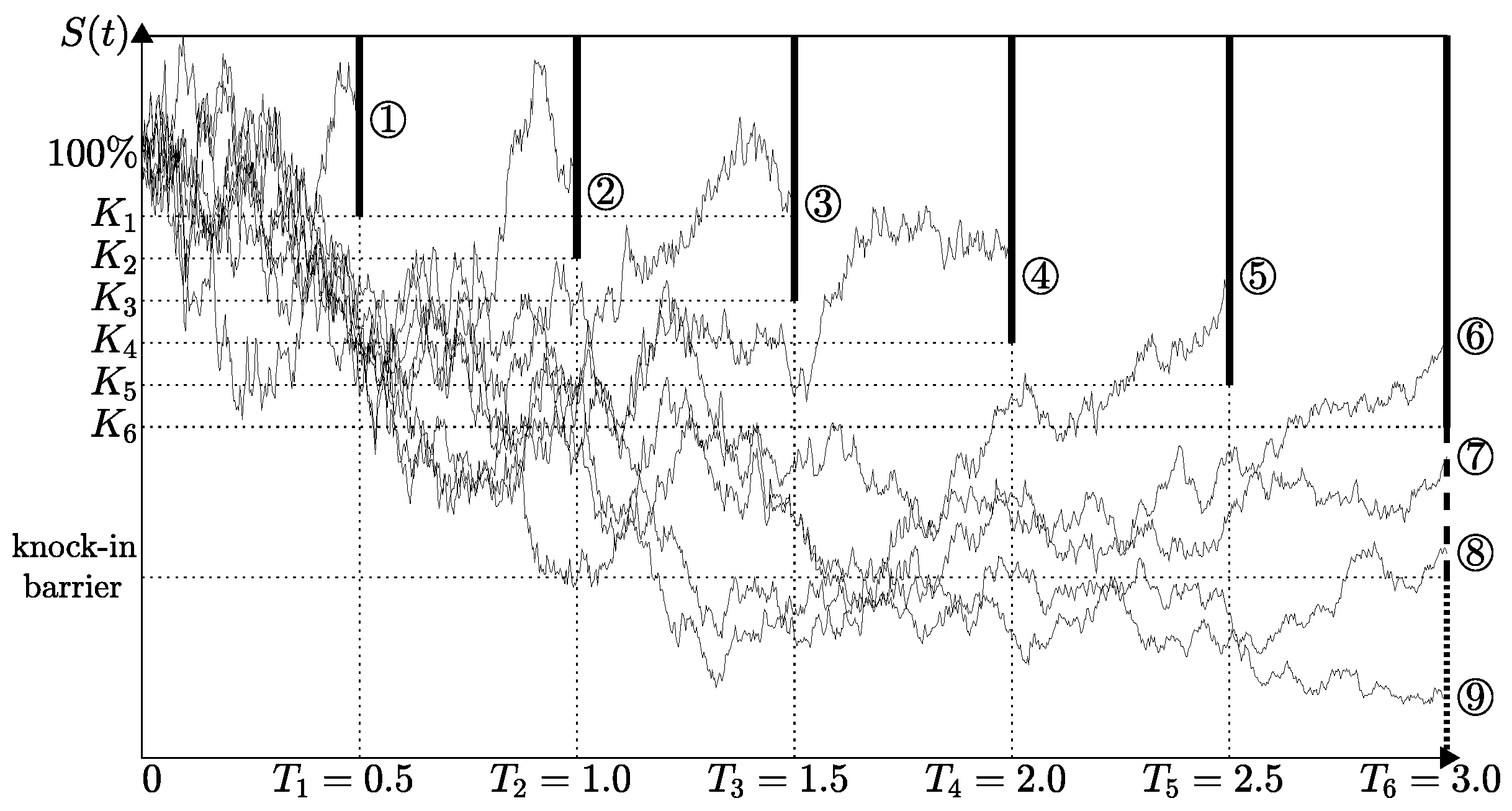
The step-down type ELS has nine possible cases as shown in Figure 2. Cases ①–⑥ represent early repayment and maturity repayment. If the repayment terms are satisfied at the time of each repayment, the corresponding coupon is paid and the contract is closed. Case ⑦ represents the case when the dummy is paid if the stock path does not hit the knock-in barrier throughout the contract period and does not satisfy early redemptions. In the cases of ⑧ and ⑨, the principal is lost because the stock path hits the knock-in barrier.

In this paper, we consider the pricing of three-asset ELS options. Let $S_t=min(x_t,y_t,z_t)$ be the minimum of the three underlying assets. Let $u(S,\tau )$ be the solution when the asset price has been below the knock-in barrier and $v(S,\tau )$ be the solution when not. The initial payoff functions of ELS option are

$$u(S,0)=\left\{\begin{array}{cc}(S_T/S_0)F,\hfill & \mathrm{if} S_T<K_6,\hfill \\ (1+c_6)F,\hfill & \mathrm{otherwise},\hfill \end{array}\right.$$

(2)

$$v(S,0)=\left\{\begin{array}{cc}(1+c_6)F,\hfill & \mathrm{if} S_T\ge K_6,\hfill \\ (1+d)F,\hfill & \mathrm{if} D<S_T<K_6,\hfill \\ (S_T/S_0)F,\hfill & \mathrm{otherwise}.\hfill \end{array}\right.$$

(3)

We overlay $v(S,\tau )$ with $u(S,\tau )$ under the knock-in barrier before solving $v(S,\tau )$. Figure 3 shows the schematic diagram of the differences between u and v at $\tau =2.5$. More details regarding ELS structure can be found in [20].

2.3. Solution Algorithm

First, we discretize $\mathsf{\Omega }=[0,L]\times [0,M]\times [0,N]$ with steps $h_{i-1}^x=x_i-x_{i-1},h_{j-1}^y=y_j-y_{j-1}$, and $h_{k-1}^z=z_k-z_{k-1}$. Here, $x_0=y_0=z_0=0$, $x_{N_x}=L$, $y_{N_y}=M$, and $z_{N_z}=N$. $N_x$, $N_y$, $N_z$, and $N_{\tau }$ are the numbers of grid points in the x-, y-, z-, and $\tau$-directions, respectively. $\Delta \tau =T/N_{\tau }$ is a time step size. Let $u_{ijk}^n\equiv u(x_i,y_j,$$z_k,n\Delta \tau )$ be the computational approximation of the solution, where $i=0,\dots ,N_x$, $j=0,\dots ,N_y$, $k=0,\dots ,N_z$, and $n=0,\dots ,N_{\tau }$. We use the first and second order partial derivatives at the discrete point $(x_i,y_j,z_k)$ as follows:

$$\begin{array}{ccc}\hfill {\left(D_{x}u\right)}_{ijk}& =& -\frac{h_i^x}{h_{i-1}^x(h_{i-1}^x+h_i^x)}{u}_{i-1,jk}+\frac{h_i^x-h_{i-1}^x}{h_{i-1}^x{h}_i^x}{u}_{ijk}+\frac{h_{i-1}^x}{h_i^x(h_{i-1}^x+h_i^x)}{u}_{i+1,jk},\hfill \\ \hfill {\left(D_{y}u\right)}_{ijk}& =& -\frac{h_j^y}{h_{j-1}^y(h_{j-1}^y+h_j^y)}{u}_{i,j-1,k}+\frac{h_j^y-h_{j-1}^y}{h_{j-1}^y{h}_j^y}{u}_{ijk}+\frac{h_{j-1}^y}{h_j^y(h_{j-1}^y+h_j^y)}{u}_{i,j+1,k},\hfill \\ \hfill {\left(D_{z}u\right)}_{ijk}& =& -\frac{h_k^z}{h_{k-1}^z(h_{k-1}^z+h_k^z)}{u}_{ij,k-1}+\frac{h_k^z-h_{k-1}^z}{h_{k-1}^z{h}_k^z}{u}_{ijk}+\frac{h_{k-1}^z}{h_k^z(h_{k-1}^z+h_k^z)}{u}_{ij,k+1},\hfill \\ \hfill {\left(D_{xx}u\right)}_{ijk}& =& \frac{2}{h_{i-1}^x(h_{i-1}^x+h_i^x)}{u}_{i-1,jk}-\frac{2}{h_{i-1}^x{h}_i^x}{u}_{ijk}+\frac{2}{h_i^x(h_{i-1}^x+h_i^x)}{u}_{i+1,jk},\hfill \\ \hfill {\left(D_{yy}u\right)}_{ijk}& =& \frac{2}{h_{j-1}^y(h_{j-1}^y+h_j^y)}{u}_{i,j-1,k}-\frac{2}{h_{j-1}^y{h}_j^y}{u}_{ijk}+\frac{2}{h_j^y(h_{j-1}^y+h_j^y)}{u}_{i,j+1,k},\hfill \\ \hfill {\left(D_{zz}u\right)}_{ijk}& =& \frac{2}{h_{k-1}^z(h_{k-1}^z+h_k^z)}{u}_{ij,k-1}-\frac{2}{h_{k-1}^z{h}_k^z}{u}_{ijk}+\frac{2}{h_k^z(h_{k-1}^z+h_k^z)}{u}_{ij,k+1},\hfill \\ \hfill {\left(D_{yx}u\right)}_{ijk}& =& \frac{u_{i+1,j+1,k}-u_{i-1,j+1,k}-u_{i+1,j-1,k}+u_{i-1,j-1,k}}{h_i^x{h}_j^y+h_{i-1}^x{h}_j^y+h_i^x{h}_{j-1}^y+h_{i-1}^x{h}_{j-1}^y},\hfill \\ \hfill {\left(D_{zy}u\right)}_{ijk}& =& \frac{u_{i,j+1,k+1}-u_{i,j-1,k+1}-u_{i,j+1,k-1}+u_{i,j-1,k-1}}{h_j^y{h}_k^z+h_{j-1}^y{h}_k^z+h_j^y{h}_{k-1}^z+h_{j-1}^y{h}_{k-1}^z},\hfill \\ \hfill {\left(D_{xz}u\right)}_{ijk}& =& \frac{u_{i+1,j,k+1}-u_{i+1,j,k-1}-u_{i-1,j,k+1}+u_{i-1,j,k-1}}{h_k^z{h}_i^x+h_{k-1}^z{h}_i^x+h_k^z{h}_{i-1}^x+h_{k-1}^z{h}_{i-1}^x}.\hfill \end{array}$$

We apply the homogenous Dirichlet boundary condition at $x=0$, $y=0$, and $z=0$; and zero Neumann boundary condition at $x=L$, $y=M$, and $z=N$ [21]. That is,

$$\begin{array}{ccc}\hfill u_{0jk}^n& =& 0,\mathrm{for}1\le j\le N_y,1\le k\le N_z,\hfill \\ \hfill u_{i0k}^n& =& 0,\mathrm{for}1\le i\le N_x,1\le k\le N_z,\hfill \\ \hfill u_{ij0}^n& =& 0,\mathrm{for}1\le i\le N_x,1\le j\le N_y,\hfill \\ \hfill u_{N_{x}jk}^n& =& u_{N_x-1,jk}^n,\mathrm{for}1\le j\le N_y-1,1\le k\le N_z-1,\hfill \\ \hfill u_{i{N}_{y}k}^n& =& u_{i,N_y-1,k}^n,\mathrm{for}1\le i\le N_x,1\le k\le N_z-1,\hfill \\ \hfill u_{ij{N}_z}^n& =& u_{ij,N_z-1}^n,\mathrm{for}1\le i\le N_x,1\le j\le N_y.\hfill \end{array}$$

We first solve Equation (1) explicitly with considering the knock-in event. For $i=1,\dots ,N_x-1$, $j=1,\dots ,N_y-1$, and $k=1,\dots ,N_z-1$,

$$\begin{array}{ccc}\hfill u_{ijk}^{n+1}& =& u_{ijk}^n+\Delta \tau \left(A_{ijk,1}{u}_{i,j-1,k-1}^n+A_{ijk,2}{u}_{i-1,j,k-1}^n+A_{ijk,3}{u}_{ij,k-1}^n+A_{ijk,4}{u}_{i+1,j,k-1}^n\right.\hfill \\ & & +A_{ijk,5}{u}_{i,j+1,k-1}^n+A_{ijk,6}{u}_{i-1,j-1,k}^n+A_{ijk,7}{u}_{i,j-1,k}^n+A_{ijk,8}{u}_{i+1,j-1,k}^n+A_{ijk,9}{u}_{i-1,jk}^n\hfill \\ & & +A_{ijk,10}{u}_{ijk}^n+A_{ijk,11}{u}_{i+1,jk}^n+A_{ijk,12}{u}_{i-1,j+1,k}^n+A_{ijk,13}{u}_{i,j+1,k}^n+A_{ijk,14}{u}_{i+1,j+1,k}^n\hfill \\ & & \left.+A_{ijk,15}{u}_{i,j-1,k+1}^n+A_{ijk,16}{u}_{i-1,j,k+1}^n+A_{ijk,17}{u}_{ij,k+1}^n+A_{ijk,18}{u}_{i+1,j,k+1}^n+A_{ijk,19}{u}_{i,j+1,k+1}^n\right).\hfill \end{array}$$

(4)

Here, we define $A_{ijk,m}$ for $m=1,\dots ,19$ as follows:

$$\begin{array}{ccc}\hfill A_{ijk,1}& =& \frac{{\rho }_{yz}{\sigma }_y{\sigma }_z{y}_j{z}_k}{h_j^y{h}_k^z+h_{j-1}^y{h}_k^z+h_j^y{h}_{k-1}^z+h_{j-1}^y{h}_{k-1}^z},A_{ijk,2}=\frac{{\rho }_{zx}{\sigma }_z{\sigma }_x{z}_k{x}_i}{h_k^z{h}_i^x+h_{k-1}^z{h}_i^x+h_k^z{h}_{i-1}^x+h_{k-1}^z{h}_{i-1}^x},\hfill \\ \hfill A_{ijk,3}& =& \frac{{\left({\sigma }_z{z}_k\right)}^2}{h_{k-1}^z(h_{k-1}^z+h_k^z)}-\frac{r{z}_k{h}_k^z}{h_{k-1}^z(h_{k-1}^z+h_k^z)},A_{ijk,4}=-A_{ijk,2},A_{ijk,5}=-A_{ijk,1},\hfill \\ \hfill A_{ijk,6}& =& \frac{{\rho }_{xy}{\sigma }_x{\sigma }_y{x}_i{y}_j}{h_i^x{h}_j^y+h_{i-1}^x{h}_j^y+h_i^x{h}_{j-1}^y+h_{i-1}^x{h}_{j-1}^y},A_{ijk,7}=\frac{{\left({\sigma }_y{y}_j\right)}^2}{h_{j-1}^y(h_{j-1}^y+h_j^y)}-\frac{r{y}_j{h}_j^y}{h_{j-1}^y(h_{j-1}^y+h_j^y)},\hfill \\ \hfill A_{ijk,8}& =& -A_{ijk,6},A_{ijk,9}=\frac{{\left({\sigma }_x{x}_i\right)}^2}{h_{i-1}^x(h_{i-1}^x+h_i^x)}-\frac{r{x}_i{h}_i^x}{h_{i-1}^x(h_{i-1}^x+h_i^x)},\hfill \\ \hfill A_{ijk,10}& =& r{x}_i\frac{h_i^x-h_{i-1}^x}{h_{i-1}^x{h}_i^x}+r{y}_j\frac{h_j^y-h_{j-1}^y}{h_{j-1}^y{h}_j^y}+r{z}_k\frac{h_k^z-h_{k-1}^z}{h_{k-1}^z{h}_k^z}-\frac{{\left({\sigma }_x{x}_i\right)}^2}{h_{i-1}^x{h}_i^x}-\frac{{\left({\sigma }_y{y}_j\right)}^2}{h_{j-1}^y{h}_j^y}-\frac{{\left({\sigma }_z{z}_k\right)}^2}{h_{k-1}^z{h}_k^z}-r,\hfill \\ \hfill A_{ijk,11}& =& \frac{{\left({\sigma }_x{x}_i\right)}^2}{h_i^x(h_{i-1}^x+h_i^x)}+\frac{r{x}_i{h}_{i-1}^x}{h_i^x(h_{i-1}^x+h_i^x)},A_{ijk,12}=-A_{ijk,6},\hfill \\ \hfill A_{ijk,13}& =& \frac{{\left({\sigma }_y{y}_j\right)}^2}{h_i^y(h_{j-1}^y+h_j^y)}+\frac{r{y}_j{h}_{j-1}^y}{h_j^y(h_{j-1}^y+h_j^y)},A_{ijk,14}=A_{ijk,6},A_{ijk,15}=-A_{ijk,1},A_{ijk,16}=-A_{ijk,2},\hfill \\ \hfill A_{ijk,17}& =& \frac{{\left({\sigma }_z{z}_k\right)}^2}{h_k^z(h_{k-1}^z+h_k^z)}+\frac{r{z}_k{h}_{k-1}^z}{h_k^z(h_{k-1}^z+h_k^x)},A_{ijk,18}=A_{ijk,2},A_{ijk,19}=A_{ijk,1}.\hfill \end{array}$$

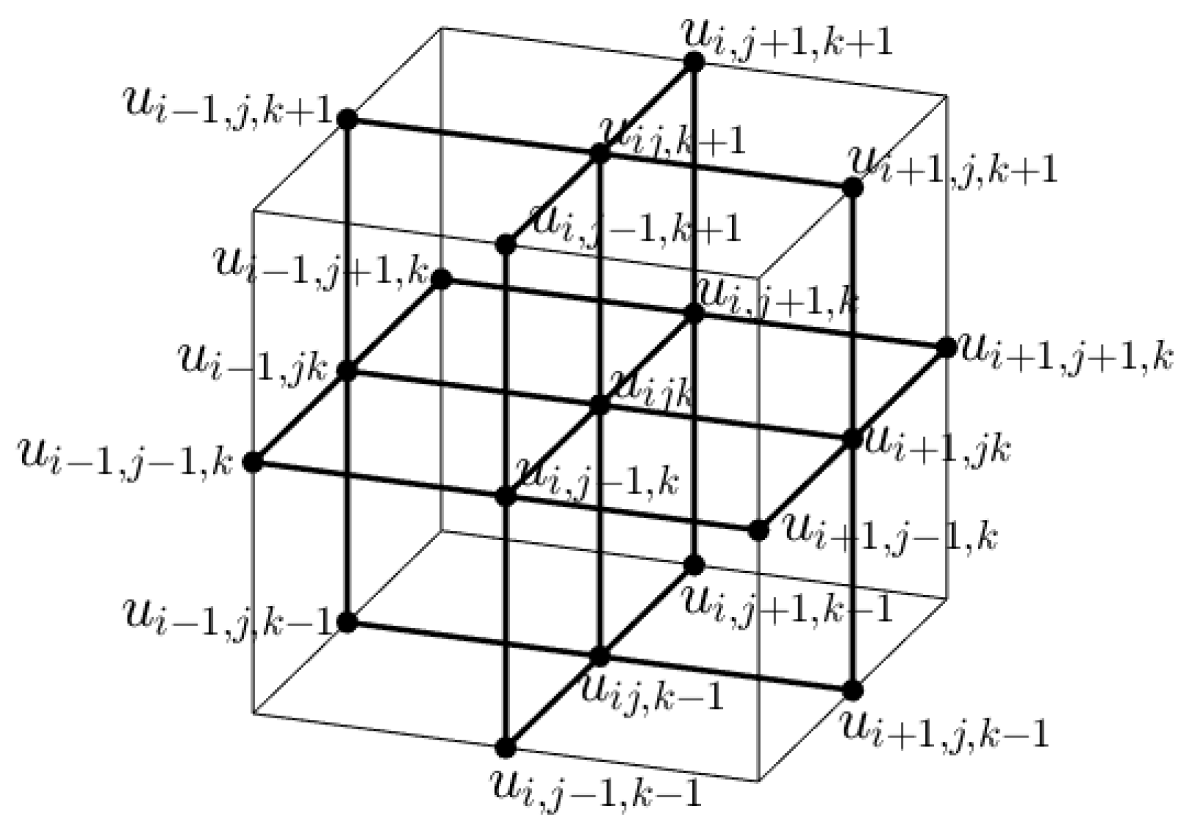
Figure 4 illustrates the 19-point discrete stencil for updating $u_{ijk}^{n+1}$.

Next, we set $v^{n+1}$ at the knock-in-barrier with $u^{n+1}$ and use it as the Dirichlet boundary condition. s is where the stock price is equal to the knock-in barrier.

$$\begin{array}{ccc}\hfill v_{sjk}^n& =& u_{sjk}^n, \mathrm{for} s\le j\le N_y,s\le k\le N_z,\hfill \\ \hfill v_{isk}^n& =& u_{isk}^n, \mathrm{for} s\le i\le N_x,s\le k\le N_z,\hfill \\ \hfill v_{ijs}^n& =& u_{ijs}^n, \mathrm{for} s\le i\le N_x,s\le j\le N_y.\hfill \end{array}$$

The homogeneous Neumann boundary condition is applied at $x=L$, $y=M$, $z=N$:

$$\begin{array}{ccc}\hfill v_{N_{x}jk}^n& =& v_{N_x-1,jk}^n, \mathrm{for} 1\le j\le N_y-1,1\le k\le N_z-1,\hfill \\ \hfill v_{i{N}_{y}k}^n& =& v_{i,N_y-1,k}^n, \mathrm{for} 1\le i\le N_x,1\le k\le N_z-1,\hfill \\ \hfill v_{ij{N}_z}^n& =& v_{ij,N_z-1}^n, \mathrm{for} 1\le i\le N_x,1\le j\le N_y.\hfill \end{array}$$

For $i=s+1,\dots ,N_x-1$, $j=s+1,\dots ,N_y-1$, $k=s+1,\dots ,N_z-1$, we solve the following

$$\begin{array}{ccc}\hfill v_{ijk}^{n+1}& =& v_{ijk}^n+\Delta \tau \left(A_{ijk,1}{v}_{i,j-1,k-1}^n+A_{ijk,2}{v}_{i-1,j,k-1}^n+A_{ijk,3}{v}_{ij,k-1}^n+A_{ijk,4}{v}_{i+1,j,k-1}^n\right.\hfill \\ & & +A_{ijk,5}{v}_{i,j+1,k-1}^n+A_{ijk,6}{v}_{i-1,j-1,k}^n+A_{ijk,7}{v}_{i,j-1,k}^n+A_{ijk,8}{v}_{i+1,j-1,k}^n+A_{ijk,9}{v}_{i-1,jk}^n\hfill \\ & & +A_{ijk,10}{v}_{ijk}^n+A_{ijk,11}{v}_{i+1,jk}^n+A_{ijk,12}{v}_{i-1,j+1,k}^n+A_{ijk,13}{v}_{i,j+1,k}^n+A_{ijk,14}{v}_{i+1,j+1,k}^n\hfill \\ & & \left.+A_{ijk,15}{v}_{i,j-1,k+1}^n+A_{ijk,16}{v}_{i-1,j,k+1}^n+A_{ijk,17}{v}_{ij,k+1}^n+A_{ijk,18}{v}_{i+1,j,k+1}^n+A_{ijk,19}{v}_{i,j+1,k+1}^n\right).\hfill \end{array}$$

(5)

2.4. Weak Condition of Time Step

In this section, we derive the weak conditions of time step under the fully explicit scheme for Equation (4). Since all coefficients of $u_{ijk}^n$ in Equation (4) are positive, namely,

$$\begin{array}{ccc}\hfill A_{ijk,10}& +& \frac{1}{\Delta \tau }\hfill \\ & & =x_i\frac{h_i^x-h_{i-1}^x}{h_{i-1}^x{h}_i^x}+r{y}_j\frac{h_j^y-h_{j-1}^y}{h_{j-1}^y{h}_j^y}+r{z}_k\frac{h_k^z-h_{k-1}^z}{h_{k-1}^z{h}_k^z}-\frac{{\left({\sigma }_x{x}_i\right)}^2}{h_{i-1}^x{h}_i^x}-\frac{{\left({\sigma }_y{y}_j\right)}^2}{h_{j-1}^y{h}_j^y}-\frac{{\left({\sigma }_z{z}_k\right)}^2}{h_{k-1}^z{h}_k^z}-r+\frac{1}{\Delta \tau }>0,\hfill \end{array}$$

(6)

we will use increasing space step sizes, i.e., $h_{i-1}^x\le h_i^x,h_{j-1}^y\le h_j^y,h_{k-1}^z\le h_k^z$ for some large $i,j,k$. Then, we write Equation (6) as follows:

$$\begin{array}{c}\hfill \frac{1}{\Delta \tau }>\frac{{\left({\sigma }_x{x}_i\right)}^2}{h_{i-1}^x{h}_i^x}+\frac{{\left({\sigma }_y{y}_j\right)}^2}{h_{j-1}^y{h}_j^y}+\frac{{\left({\sigma }_z{z}_k\right)}^2}{h_{k-1}^z{h}_k^z}+r.\end{array}$$

Let $h_{min}=min\{h_i^x,h_j^y,h_k^z\}$ for some $i,j,k$, then

$$\begin{array}{c}\hfill \Delta \tau <\frac{h_{min}^2}{{\left({\sigma }_x{x}_i\right)}^2+{\left({\sigma }_y{y}_j\right)}^2+{\left({\sigma }_z{z}_k\right)}^2+r{h}_{min}^2}.\end{array}$$

Due to $x_{N_x}=L$, $y_{N_y}=M$, and $z_{N_z}=N$, we have

$$\begin{array}{c}\hfill \Delta \tau <\frac{h_{min}^2}{{\left({\sigma }_{x}L\right)}^2+{\left({\sigma }_{y}M\right)}^2+{\left({\sigma }_{z}N\right)}^2+r{h}_{min}^2}.\end{array}$$

(7)

3. Numerical Experiments

In this section, we demonstrate the performance of the proposed algorithm using numerical experiments with three types of ELS and comparison with MCS. For all the tests, we use the same parameters: risk-free interest rate $r=0.03$, volatilities ${\sigma }_x={\sigma }_y={\sigma }_z=0.3$, correlation ${\rho }_{xy}={\rho }_{yz}={\rho }_{zx}=0.5$, the computational domain $\mathsf{\Omega }=[0,L]\times [0,M]\times [0,N]$ with $L=M=N=150$, coupon rates $[c_1,c_2,c_3,c_4,c_5,c_6]=[0.05,0.1,0.15,0.2,0.25,0.3]$, knock-in-barrier $D=50$, face value $F=100$, and dummy rate $d=0.27$. We test three types of ELS, which have the same parameters as previously mentioned except for strike percentages. The first type of ELS has strike percentages $[K_1,K_2,K_3,K_4,K_5,K_6]=[90,90,90,90,90,90]$, the second type has $[K_1,K_2,K_3,K_4,K_5,K_6]=[95,95,90,90,85,85]$, and the third type has $[K_1,K_2,K_3,K_4,K_5,K_6]=[95,90,85,80,75,70]$. In other words, the first type of ELS has the same strike percentages at all early repayment dates, the second type has the three different strike percentages, and the last type has a different strike percentage at all repayment dates. Computations were performed on a 2.7 GHz Intel (Intel, Santa Clara, CA, USA) PC with 16 GB of RAM loaded with C language for FDM and with MATLAB 2019b (MathWorks, Natick, MA, USA) for MCS.

We propose a systematic grid generation for fast FDM for pricing a three-asset ELS as shown in Figure 5a.

The generation of the non-uniform grid is as follows: Let h be a given basic grid size.

$$\begin{array}{c}\hfill {\mathsf{\Omega }}_1=\{0,0.5D,D-h,D,D+h,S_0\},\end{array}$$

which is the fixed grid points. Let H be the grid size between $D+h$ and $K_6-0.5h$. If we want H to be approximately $\tilde{H}$, then $H=(K_6-1.5h-D)/\left[(K_6-1.5h-D)/\tilde{H}+1\right]$, where $\left[\right]$ is the floor function. Then, we have the grid point set between $D+h$ and $K_6-0.5h$:

$$\begin{array}{ccc}\hfill {\mathsf{\Omega }}_2& =& \{D+h+H,D+h+2H,\cdots ,K_6-0.5h\}.\hfill \end{array}$$

Additionally, we have

$$\begin{array}{ccc}\hfill {\mathsf{\Omega }}_3& =& \{K_6+0.5h,K_6+1.5h,\dots ,S_0-0.5h,S_0+0.5h\},\hfill \\ \hfill {\mathsf{\Omega }}_4& =& \{S_0+0.5h+d,S_0+0.5h+3d,\cdots ,L\},\hfill \end{array}$$

where $d=2(L-S_0-0.5h)/\left[m(m+1)\right]$ for some integer m, which implies the gap between points next to each other forms an arithmetic sequence. See Figure 5b–e for the schematic illustration of ${\mathsf{\Omega }}_1,{\mathsf{\Omega }}_2,{\mathsf{\Omega }}_3,$ and ${\mathsf{\Omega }}_4$, respectively. Finally, we have a grid set for the x-axis:

$$\begin{array}{c}\hfill {\mathsf{\Omega }}_x={\mathsf{\Omega }}_1\cup {\mathsf{\Omega }}_2\cup {\mathsf{\Omega }}_3\cup {\mathsf{\Omega }}_4.\end{array}$$

Let ${\mathsf{\Omega }}_y={\mathsf{\Omega }}_x$ and ${\mathsf{\Omega }}_z={\mathsf{\Omega }}_x$, therefore, the discrete domain is ${\mathsf{\Omega }}_x\times {\mathsf{\Omega }}_y\times {\mathsf{\Omega }}_z$.

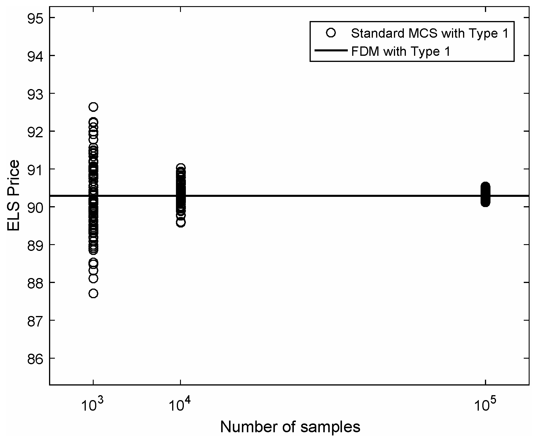
Now, we present comparison tests for three types of ELS using standard MCS and fast FDM. For more information regarding the numerical method of MCS for three-asset ELS pricing, refer to [22]. The first type of ELS has strike percentages $[K_1,K_2,K_3,K_4,K_5,K_6]=[90,90,90,90,90,90]$. Figure 6 shows Type 1 ELS MCS price versus the number of samples together with the result of the fast FDM. Here, we plot 100 MCS results for each case. The solid line is the result of the fast FDM.

Table 1. The price and computation time of Type 1 ELS prices with the standard Monte Carlo simulation (MCS) and the fast finite difference method (FDM).

Case	Price	CPU Time (s)
Standard MCS	90.3002	369.4568
Fast FDM	90.2910	2.3900

lists the price and computation time of Type 1 ELS with two different methods. For the standard MCS, the price and computation time are obtained with ${10}^6$ samples. For the fast FDM, the results are obtained with $h=2.5$, $\tilde{H}=2.5h$, $m=3$, and $\Delta \tau =1/1440$.

The second type of ELS has strike percentages $[K_1,K_2,K_3,K_4,K_5,K_6]=[95,95,90,90,85,85]$. Figure 7 shows the Type 2 ELS MCS price versus the number of samples together with the result of the fast FDM, which is represented by the solid line.

Table 2. Price and computation time of Type 2 ELS prices with the standard MCS and the fast FDM.

Case	Price	CPU Time (s)
Standard MCS	89.1673	386.3436
Fast FDM	89.0452	3.3280

lists the price and computation time of Type 2 ELS with two different methods. For the standard MCS, the price and computation time are obtained with ${10}^6$ samples. For the fast FDM, the results are obtained with $h=2.5$, $\tilde{H}=2.5h$, $m=3$, and $\Delta \tau =1/1440$.

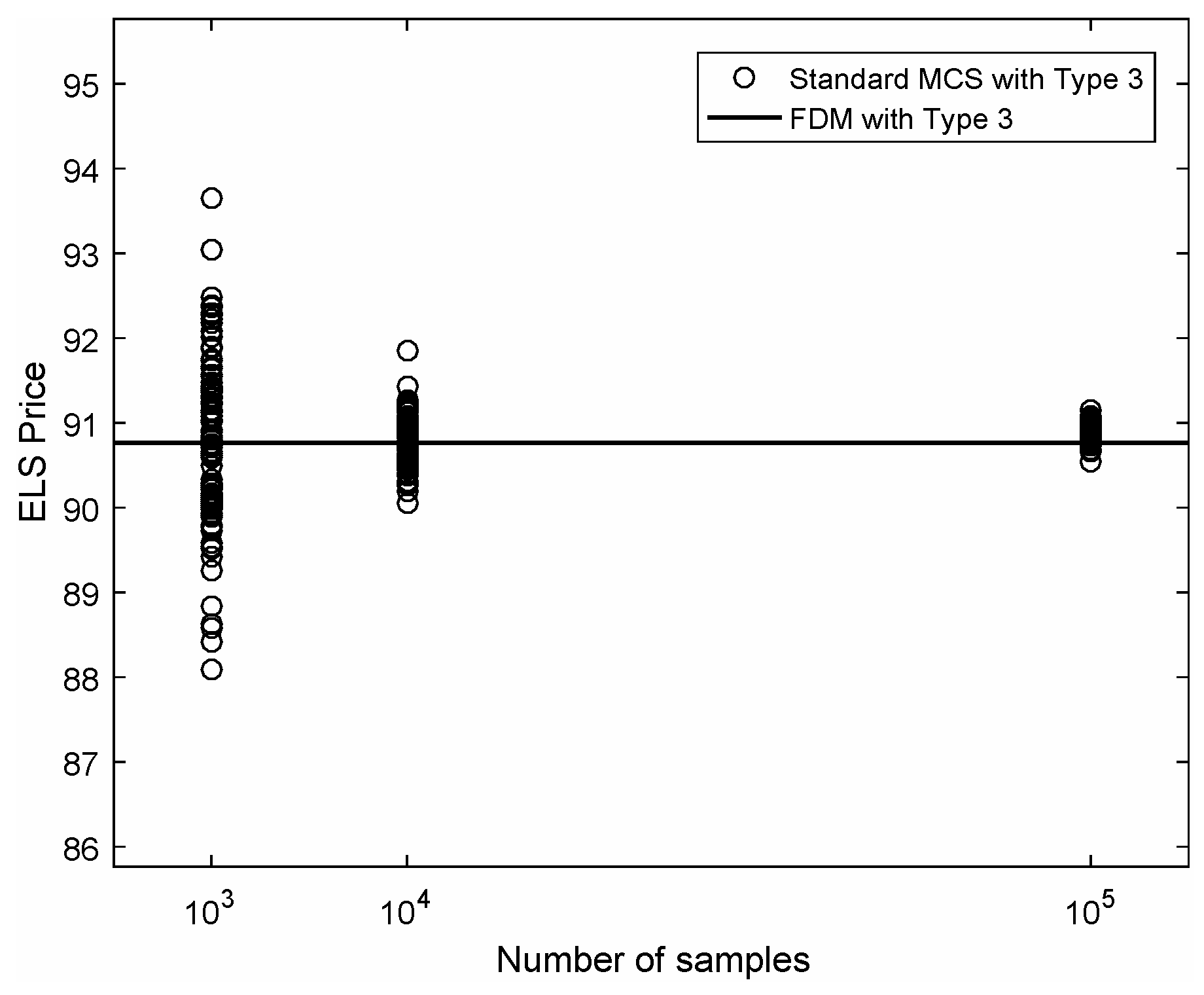
The third type of ELS has strike percentages $[K_1,K_2,K_3,K_4,K_5,K_6]=[95,90,85,80,75,70]$. Figure 8 shows the Type 3 ELS MCS price versus the number of samples together with the result of the fast FDM, which is represented by the solid line.

Table 3. Price and computation time of Type 3 ELS prices with the standard MCS and the fast FDM.

Case	Price	CPU Time (s)
Standard MCS	90.8376	369.9680
Fast FDM	90.7650	5.1090

lists the price and computation time of Type 3 ELS with two different methods. For the standard MCS, the price and computation time are obtained with ${10}^6$ samples. For the fast FDM, the results are obtained with $h=2.5$, $\tilde{H}=2.5h$, $m=3$, and $\Delta \tau =1/1440$. From these three types of ELS results, we can confirm that the proposed explicit FDM is fast and accurate.

Finally, we compare our method with the previous work [20], which used an operator splitting method (OSM) to verify that the proposed algorithm is fast and accurate. In the OSM, we solve the governing equations with multiple steps:

$$\begin{array}{c}\hfill \frac{u_{ijk}^{n+1}-u_{ijk}^n}{\Delta \tau }={\left({\mathcal{L}}_{\mathrm{BS}}^{x}u\right)}_{ijk}^{n+\frac{1}{3}}+{\left({\mathcal{L}}_{\mathrm{BS}}^{y}u\right)}_{ijk}^{n+\frac{2}{3}}+{\left({\mathcal{L}}_{\mathrm{BS}}^{z}u\right)}_{ijk}^{n+1},\end{array}$$

(8)

where ${\mathcal{L}}_{\mathrm{BS}}^x$, ${\mathcal{L}}_{\mathrm{BS}}^y$, and ${\mathcal{L}}_{\mathrm{BS}}^z$ are given as

$$\begin{array}{ccc}\hfill {\left({\mathcal{L}}_{\mathrm{BS}}^{x}u\right)}_{ijk}^{n+\frac{1}{3}}& =& \frac{{\left({\sigma }_x{x}_i\right)}^2}{2}{D}_{xx}{u}_{ijk}^{n+\frac{1}{3}}+r{x}_i{D}_x{u}_{ijk}^{n+\frac{1}{3}}+\frac{1}{3}{\sigma }_x{\sigma }_y{\rho }_{xy}{x}_i{y}_j{D}_{xy}{u}_{ijk}^n\hfill \\ & & +\frac{1}{3}{\sigma }_y{\sigma }_z{\rho }_{yz}{y}_j{z}_k{D}_{yz}{u}_{ijk}^n+\frac{1}{3}{\sigma }_z{\sigma }_x{\rho }_{zx}{z}_k{x}_i{D}_{zx}{u}_{ijk}^n-\frac{1}{3}r{u}_{ijk}^{n+\frac{1}{3}},\hfill \end{array}$$

(9)

$$\begin{array}{ccc}\hfill {\left({\mathcal{L}}_{\mathrm{BS}}^{y}u\right)}_{ijk}^{n+\frac{2}{3}}& =& \frac{{\left({\sigma }_y{y}_j\right)}^2}{2}{D}_{yy}{u}_{ijk}^{n+\frac{2}{3}}+r{y}_j{D}_y{u}_{ijk}^{n+\frac{2}{3}}+\frac{1}{3}{\sigma }_x{\sigma }_y{\rho }_{xy}{x}_i{y}_j{D}_{xy}{u}_{ijk}^{n+\frac{1}{3}}\hfill \\ & & +\frac{1}{3}{\sigma }_y{\sigma }_z{\rho }_{yz}{y}_j{z}_k{D}_{yz}{u}_{ijk}^{n+\frac{1}{3}}+\frac{1}{3}{\sigma }_z{\sigma }_x{\rho }_{zx}{z}_k{x}_i{D}_{zx}{u}_{ijk}^{n+\frac{1}{3}}-\frac{1}{3}r{u}_{ijk}^{n+\frac{2}{3}},\hfill \end{array}$$

(10)

$$\begin{array}{ccc}\hfill {\left({\mathcal{L}}_{\mathrm{BS}}^{z}u\right)}_{ijk}^{n+1}& =& \frac{{\left({\sigma }_z{z}_k\right)}^2}{2}{D}_{zz}{u}_{ijk}^{n+1}+r{z}_k{D}_z{u}_{ijk}^{n+1}+\frac{1}{3}{\sigma }_x{\sigma }_y{\rho }_{xy}{x}_i{y}_j{D}_{xy}{u}_{ijk}^{n+\frac{2}{3}}\hfill \\ & & +\frac{1}{3}{\sigma }_y{\sigma }_z{\rho }_{yz}{y}_j{z}_k{D}_{yz}{u}_{ijk}^{n+\frac{2}{3}}+\frac{1}{3}{\sigma }_z{\sigma }_x{\rho }_{zx}{z}_k{x}_i{D}_{zx}{u}_{ijk}^{n+\frac{2}{3}}-\frac{1}{3}r{u}_{ijk}^{n+1}.\hfill \end{array}$$

(11)

We solve the below equations, one by one, using the Thomas algorithm:

$$\begin{array}{c}\hfill \frac{u_{ijk}^{n+\frac{1}{3}}-u_{ijk}^n}{\Delta \tau }={\left({\mathcal{L}}_{\mathrm{BS}}^{x}u\right)}_{ijk}^{n+\frac{1}{3}},\frac{u_{ijk}^{n+\frac{2}{3}}-u_{ijk}^{n+\frac{1}{3}}}{\Delta \tau }={\left({\mathcal{L}}_{\mathrm{BS}}^{y}u\right)}_{ijk}^{n+\frac{2}{3}},\frac{u_{ijk}^{n+1}-u_{ijk}^{n+\frac{2}{3}}}{\Delta \tau }={\left({\mathcal{L}}_{\mathrm{BS}}^{z}u\right)}_{ijk}^{n+1}.\end{array}$$

(12)

For more details about the numerical procedure, please refer to [20]. For comparison, we take the Type 3 ELS with all the same parameter values. The absolute errors of the computed option values with the reference MCS value are $0.0726$ and $0.3409$ for the proposed method and the OSM, respectively. We achieve a more accurate result. Furthermore, the CPU time for the OSM is $74.2174$, which is about 14 times longer than the proposed method.

4. Conclusions

In this paper, we presented a super-fast computational algorithm for three-asset ELS using FDM, which is the most popular investment product in South Korea. To overcome the limitations of dimension for FDM, we developed a systematic non-uniform grid with an explicit Euler scheme and an optimal implementation of the algorithm. The computational time is less than 6 s, which is very fast. We performed standard ELS option pricing and compared the results from the fast FDM with the ones from MCS. The computational results confirmed the superiority and practicality of the proposed algorithm. We used the BS model, which assumed interest rates and volatility as constant for simplicity. However, this assumption can cause serious errors when calculating prices as they are not constants in real financial markets. Moreover, there is a limitation of the BS model because the Brownian motion oriented asset pricing is not adequate in the case where the stochastic processes’ finite dimensional distributions’ tails are heavier, compared to the tails of the elliptic distributions. For future work, we will consider the Heston model [23] and the Heston–Hull–White model [24], which assume the interest rates and volatility as variable and the case that the stochastic processes’ finite dimensional distributions’ tails are heavier.

References

- Deng, G.; Mallett, J.; McCann, C. Modeling autocallable structured products. In Derivatives and Hedge Funds; Palgrave Macmillan: London, UK, 2016; pp. 323–344. [Google Scholar]
- Haugh, M.B.; Kogan, L. Pricing American options: A duality approach. Oper. Res. 2004, 52, 258–270. [Google Scholar] [CrossRef]
- Pagés, G. The Monte Carlo Method and Applications to Option Pricing. In Numerical Probability; Springer: Cham, Germany, 2018; pp. 27–47. [Google Scholar]
- Moon, K.S.; Kim, H. A multi-dimensional local average lattice method for multi-asset models. Quant. Finance 2013, 13, 873–884. [Google Scholar] [CrossRef]
- Cen, Z.; Le, A. A robust and accurate finite difference method for a generalized Black–Scholes equation. J. Comput. Appl. Math. 2011, 235, 3728–3733. [Google Scholar] [CrossRef] [Green Version]
- Jeong, D.; Yoo, M.; Kim, J. Finite difference method for the Black–Scholes equation without boundary conditions. Comput. Econ. 2018, 51, 961–972. [Google Scholar] [CrossRef]
- Gulen, S.; Popescu, C.; Sari, M. A New Approach for the Black–Scholes Model with Linear and Nonlinear Volatilities. Mathematics 2019, 7, 760. [Google Scholar] [CrossRef] [Green Version]
- Zhang, R.; Song, H.; Luan, N. Weak Galerkin finite element method for valuation of American options. Front. Math. China 2014, 9, 455–476. [Google Scholar] [CrossRef]
- Mehrdoust, F. A new hybrid Monte Carlo simulation for Asian options pricing. J. Stat. Comput. Simul. 2015, 85, 507–516. [Google Scholar] [CrossRef]
- Wang, S. A novel fitted finite volume method for the Black–Scholes equation governing option pricing. IMA J. Numer. Anal. 2014, 24, 699–720. [Google Scholar] [CrossRef]
- Ma, J. A stochastic correlation model with mean reversion for pricing multi-asset options. Asia-Pac Financ Markets 2009, 16, 97–109. [Google Scholar] [CrossRef]
- Leentvaar, C.C.W.; Oosterlee, C.W. Pricing multi-asset options with sparse grids and fourth order finite differences. In Pricing Multi-Asset Options with Sparse Grids and Fourth Order Finite Differences; de Castro, A.B., Gómez, D., Quintela, P., Salgado, P., Eds.; Springer: Berlin/Heidelberg, Germany, 2007; pp. 809–814. [Google Scholar]
- Ikonen, S.; Toivanen, J. Operator splitting methods for American option pricing. Appl. Math. Lett. 2004, 17, 809–814. [Google Scholar] [CrossRef] [Green Version]
- Heinecke, A.; Schraufstetter, S.; Bungartz, H.J. A highly parallel Black–Scholes solver based on adaptive sparse grids. Int. J. Comput. Math. 2012, 89, 1212–1238. [Google Scholar] [CrossRef]
- Guillaume, T. Autocallable structured products. J. Deriv. 2015, 22, 73–94. [Google Scholar] [CrossRef]
- Guillaume, T. On the multidimensional Black–Scholes partial differential equation. Ann. Oper. Res. 2019, 281, 229–251. [Google Scholar] [CrossRef]
- Yoo, M.; Jeong, D.; Seo, S.; Kim, J. A comparison study of explicit and implicit numerical methods for the equity-linked securities. Honam Math. J. 2015, 37, 441–455. [Google Scholar] [CrossRef] [Green Version]
- O’Sullivan, S.; O’Sullivan, C. On the acceleration of explicit finite difference methods for option pricing. Quant. Finance 2011, 11, 1177–1191. [Google Scholar] [CrossRef]
- Boyle, P.P.; Tian, Y. An explicit finite difference approach to the pricing of barrier options. Appl. Math. Finance 1998, 5, 17–43. [Google Scholar] [CrossRef]
- Kim, J.; Kim, T.; Jo, J.; Choi, Y.; Lee, S.; Hwang, H.; Yoo, M.; Jeong, D. A practical finite difference method for the three-dimensional Black–Scholes equation. Eur. J. Oper. Res. 2016, 252, 183–190. [Google Scholar] [CrossRef]
- Choi, Y.; Jeong, D.; Kim, J.; Kim, Y.R.; Lee, S.; Seo, S.; Yoo, M. Robust and accurate method for the Black–Scholes equations with payoff-consistent extrapolation. Commun. Korean Math. Soc. 2015, 30, 297–311. [Google Scholar] [CrossRef] [Green Version]
- Jo, J.; Kim, Y. Comparison of numerical schemes on multi-dimensional Black–Scholes equations. Bull. Korean Math. Soc. 2013, 50, 2035–2051. [Google Scholar] [CrossRef] [Green Version]
- Heston, S.L. A closed-form solution for options with stochastic volatility with applications to bond and currency options. Rev. Financ. Stud. 1993, 6, 327–343. [Google Scholar] [CrossRef] [Green Version]
- Ullah, M.Z. Numerical Solution of Heston–Hull–White Three-Dimensional PDE with a High Order FD Scheme. Mathematics 2019, 7, 704. [Google Scholar] [CrossRef] [Green Version]
Figure 1.
Payoff structure of a one-asset step-down ELS.
Figure 2.
Nine cases of random stock path for the step-down type ELS.
Figure 3.
Schematic illustration of u and v at = 2.5.
Figure 4.
The 19-point discrete stencil for .
Figure 5.
(a) Schematic illustration of the suggested grid . (b–e) are schematic illustrations of , , , and .
Figure 6.
Type 1 equity-linked securities (ELS) price versus the number of samples. Here, we plot 100 simulation results for each case.
Figure 7.
The type 2 ELS price versus the number of samples. Here, we plot 100 simulation results for each case.
Figure 8.
Type 3 ELS price versus the number of samples. Here, we plot 100 simulation results for each case.