Predictive Modeling the Free Hydraulic Jumps Pressure through Advanced Statistical Methods

Abstract

Pressure fluctuations beneath hydraulic jumps potentially endanger the stability of stilling basins. This paper deals with the mathematical modeling of the results of laboratory-scale experiments to estimate the extreme pressures. Experiments were carried out on a smooth stilling basin underneath free hydraulic jumps downstream of an Ogee spillway. From the probability distribution of measured instantaneous pressures, pressures with different probabilities could be determined. It was verified that maximum pressure fluctuations, and the negative pressures, are located at the positions near the spillway toe. Also, minimum pressure fluctuations are located at the downstream of hydraulic jumps. It was possible to assess the cumulative curves of pressure data related to the characteristic points along the basin, and different Froude numbers. To benchmark the results, the dimensionless forms of statistical parameters include mean pressures (P*_m), the standard deviations of pressure fluctuations (σ*_X), pressures with different non-exceedance probabilities (P*_k%), and the statistical coefficient of the probability distribution (N_k%) were assessed. It was found that an existing method can be used to interpret the present data, and pressure distribution in similar conditions, by using a new second-order fractional relationships for σ*_X, and N_k%. The values of the N_k% coefficient indicated a single mean value for each probability.

1. Introduction

In hydraulic jumps, the high-velocity of an incoming flow abruptly has an impact against a slower flow [1]. The classical hydraulic jump (CHJ) occurs on the smooth bed of stilling basins. A hydraulic jump is a phenomenon with non-deterministic characteristics, and for practical purposes, can be treated with the mathematical analysis approaches. Considering that the turbulent pressure nature is highly random, the analysis is mainly based on mathematical methodologies. Therefore, the stochastic characteristics of the problem should be paid attention to [2,3]. This property is a function of the turbulent characteristic of the velocity and pressure field.

Knowledge of pressure fluctuations and extreme pressures allows for a better understanding of the energy dissipation process along the hydraulic jump. Notable early studies on pressure fluctuations are such as those by Bukreyev [4], Locher [5], Schiebe [6], Abdul Khader and Elango [7], Lopardo et al. [8], Lopardo [9], Toso and Bowers [2], Farhoudi and Narayanan [10], Fiorotto and Rinaldo [11], Fiorotto and Rinaldo [12], and Armenio et al. [13].

According to Yan et al. [14], the pressure fluctuations coefficient (Cʹ_P) and peak frequencies of the spatial hydraulic jumps are higher than the classical jumps. Onitsuka et al. [15] found that roller oscillations affect the instantaneous flow depth and bed pressure. In addition, the instantaneous bed pressures are associated with free surface fluctuations. Lian et al. [16] stated that the fluctuating pressure spectrum in the rolling area follows the gravity similarity law. Lopardo and Romagnoli [17] and Lopardo [18] used Cʹ_P coefficient values to estimate the turbulence intensities close to the stilling basin bed for the low incident Froude numbers. Wang et al. [19] predicted the total pressure based upon the void fraction and velocity data, and the results were in good agreement with the experimental data. Firotto et al. [20] studied the stability of a plunge pool lining under the fully developed jets and proposed a design approach to determine the thickness of the linings. Barjastehmaleki et al. [21] investigated the statistical structure of fluctuating pressures within the stilling basins. Barjastehmaleki et al. [22] evaluated an approach for the structural design of stilling basins lining in the sealed and unsealed joints. Lopardo [9] recommended specific flow conditions to measure pressure fluctuations. According to this, the supercritical Reynolds number (Re₁) should be more than 100,000. The minimum acquisition time must be 60 seconds. The acquisition frequency can be considered between 50 and 100 Hz. The maximum length of the plastic tube between the pressure tap and transducer is equal to 55 cm with a minimum inner diameter of 5 mm.

There are some pressure estimation methodologies associated with the hydraulic jumps in the literature. Gu et al. [23] evaluated the Smoothed Particle Hydrodynamics (SPH) model to estimate the wave profile, velocity data, and energy dissipation caused by hydraulic jumps. Güven et al. [24] used neural networks to predict the pressure fluctuations on the bed of a sloping stilling basin under B-type hydraulic jump, was investigated in detail by Hager [25]. Teixeira [26] determined the extreme pressures with different non-exceedance probabilities (P*_k%) from the sample data within a stilling basin. Teixeira et al. [27] provided the cumulative curves of P*_k% for characteristic points along the hydraulic jump. Souza et al. [28] investigated the behavior of the hydraulic jump concerning the longitudinal distribution of pressures near the bottom of the basin in the low Froude number zone (Fr₁ ≤ 4.5). Prá et al. [29] investigated the influence of the vertical curve between the spillway toe and the stilling basin bed. The results showed that maximum pressure fluctuations were identified at the center of the vertical curve and assume values of 1% of the flow kinetic energy at the terminal tangency point of the curve. Novakoski et al. [30] investigated extreme pressures with different probabilities (P*_k%) on a smooth basin downstream of a stepped spillway. The results showed that the values of P*_0.1% and P*_99.9% have lower and higher values than the values observed downstream of the smooth chute, in the region near the spillway toe, respectively.

Pressure distributions along the hydraulic jumps are not described by a normal distribution [31]. The distributions of the skewness (S) and kurtosis (K) coefficients of the sample pressure data along the hydraulic jump differ significantly from the value 0, attributed to a normal distribution. This values is observed after the endpoint of the hydraulic jump at the dimensionless position X* ≈ 8. According to Marques et al. [31], the distances of pressure points can be dimensionless concerning the conjugate depths, i.e., X* = X/ (Y₂ −Y₁). Analysis of S and K coefficients displays that there are several types of distributions along hydraulic jumps. Therefore, it is difficult to estimate the pressure data with a certain probability (P*_k%). They proposed dimensionless relationships linking pressure data of P*_k% to the mean pressure (P*_m), and the standard deviation of the sample data (σ*_X). Such relationships allow us to organize the results of different flow discharges or Froude numbers and characterize the interest points in hydraulic jumps.

Generally, mean velocity and hydrostatic pressure are considered for designing a stilling basin. However, in the turbulent flow, the characteristics of the fluctuating fields of pressure and velocity may be more important than the mean values. Accordingly, the design of the stilling basin apron requires an assessment of the pressures acting upon the bottom of the basin to optimize concrete thickness. It is essential to study the instantaneous pressures beneath the hydraulic jump. There is little information about the pressure fluctuations, because it is quite difficult to measure the pressures underneath the hydraulic jump on the bed of stilling basins in the field [15]. Therefore, laboratory-scale experiments covering pressure fluctuations seem to be reasonable and necessary [32]. Indeed, the United States Bureau of Reclamation (USBR) has provided the general design criteria concerning the stilling basin length, assuming that the hydraulic jump is confined within the stilling basin. However, no indications are given to the different types of hydraulic jump, pressure regime, and forces on the bed of stilling basins [33].

Therefore, the main aim of the present study is to measure and provide useful information about the pressure fluctuations. To do this, the experimental results are compared with those obtained on the bed of smooth basins in the literature. Many laboratory-scale experiments were designed to simulate the flow patterns downstream of an Ogee spillway, cascading into a USBR type I stilling basin, and measuring the pressure fluctuations with a frequency of 20 Hz along the longitudinal axis of the basin. The focus of this study is the mathematical analysis of the extreme pressures distribution at the bottom of a smooth stilling basin for the incident Froude numbers (Fr₁) ranging from 7.12 to 9.46. New relationships will be proposed for the dimensionless standard deviation (σ*_X), and the statistical coefficient of the probability distribution (N_k%) to estimate the extreme pressures with different non-exceedance probabilities (P*_k%).

2. Materials and Methods

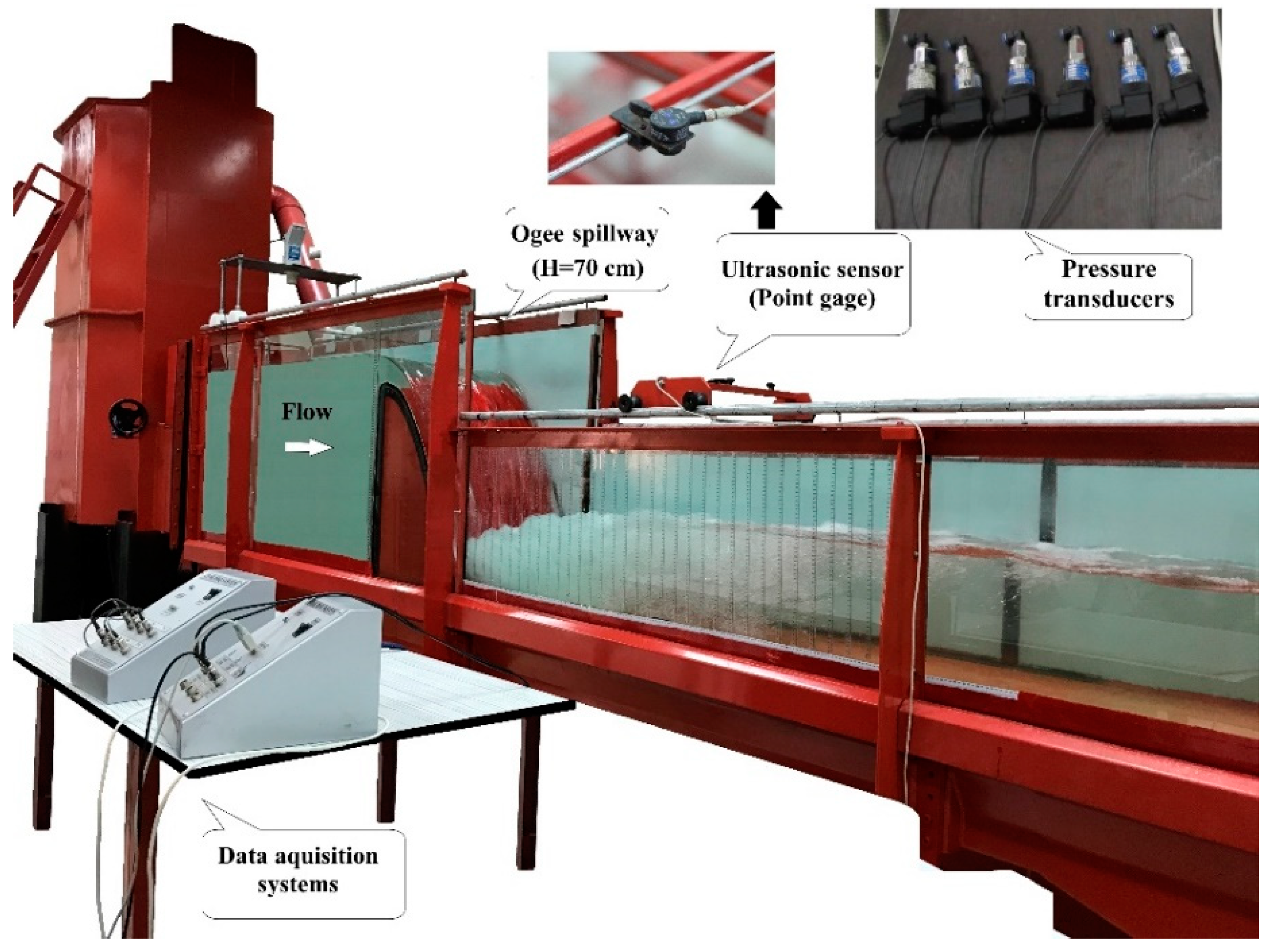
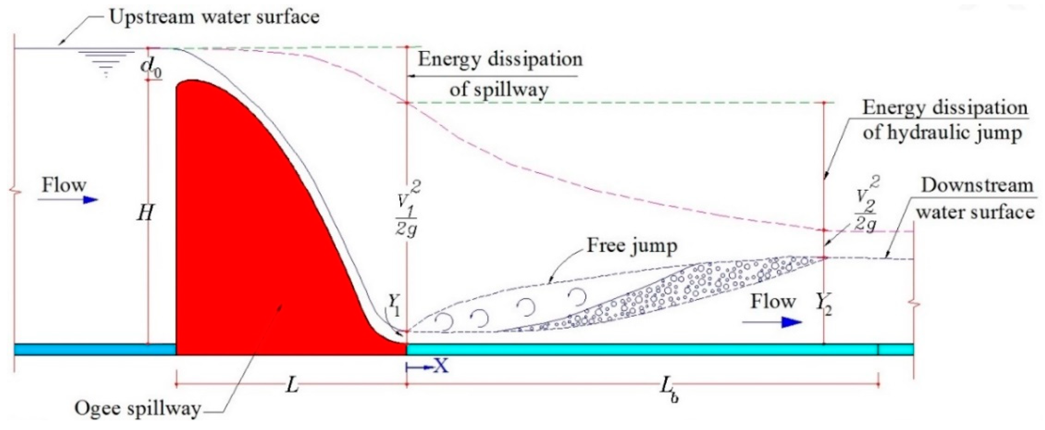
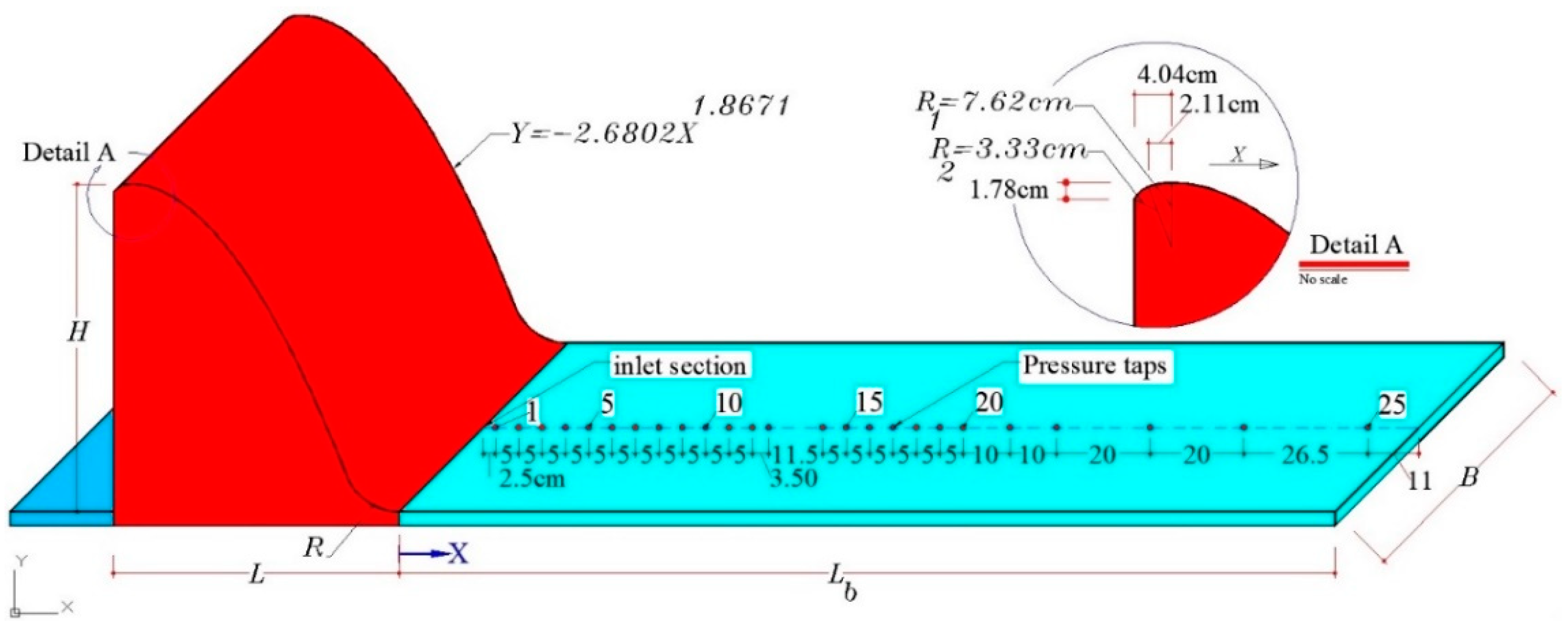
2.1. Experimental Setup

Pressure patterns along free hydraulic jumps acting on the bottom of the USBR Type I stilling basin (smooth bed) downstream of an Ogee spillway, were investigated using a laboratory model (Figure 1). The experiments were conducted in a laboratory Plexiglas-walled flume with 50 cm width, 60 cm height, and 10 m length in the hydraulic laboratory at the University of Tabriz, Iran. The flume bed was horizontal. An Ogee spillway with 70 cm height (H), and 61 cm length (L) was equipped with a Type I stilling basin according to the USBR criteria [34].

The length of the USBR Type I stilling basin (L_b) was considered 200 cm [35]. The basin width (B) was equal to the flume width (50 cm). The radius of the vertical curve (R) at the spillway toe was 12 cm. There was a head tank with 250 cm height to stabilize the flow upstream of the spillway. A hinged weir downstream of the flume was used to control the position of the supercritical depth (Y₁) at the spillway toe. The sequent depth (Y₂) was measured by an ultrasonic sensor, with an operating in the range of 10 to 100 cm, and the accuracy of the nominal value the manufacture ±0.1 mm. For the classical hydraulic jump (CHJ), the most relevant parameter is the incident Froude number (Fr₁). The Froude number characterizes the balance between inertial and gravitational forces. A value of Fr₁ > 1 indicates the supercritical flow, and vice versa for Fr₁ < 1 [36,37,38].

$${\mathrm{Fr}}_1=\frac{V_1}{\sqrt{g\times Y_1}}$$

(1)

$$V_1=\sqrt{2g\times (Z-\frac{d_0}{2})}$$

(2)

where V₁ is the mean supercritical velocity; d₀ is the hydraulic head upstream of the spillway crest; Z is the total water depth upstream of the spillway (Z = H + d₀); and g is the gravitational acceleration. The values of Y₁ are calculated using the continuity low (Y₁ = q/V₁), where q is the flow discharge per unit width. Figure 2 displays some experimental parameters. Figure 3 shows the distribution of pressure taps along the centerline of the stilling basin. The flow discharge (Q) was measured with an ultrasonic flowmeter. Experiments were carried out with different flow discharges in the range of 33 to 60.4 L/s.

Table 1. Experimental parameters along the hydraulic jumps.

Q (L/s)	Y1 (cm)	Y2 (cm)	V1 (m/s)	Fr1 (−)
60.4	3.04	27.55	3.89	7.12
55.0	2.78	26.49	3.88	7.44
52.7	2.66	26.05	3.88	7.59
47.5	2.41	24.87	3.87	7.96
43.0	2.18	23.70	3.86	8.34
33.0	1.68	20.65	3.84	9.46

presents the range of some experimental parameters along the hydraulic jumps.

To measure the instantaneous pressure data, 25 pressure taps were installed at the bottom, along the centerline of the stilling basin. Afterward, these data were converted into electrical signals by pressure transducers via a 6-channel digital board. In this study, the transparent plastic tubes were used with an inner diameter of 3 mm, and the maximum lengths of 200 cm. The six Atek transducers (model BCT–110) had an operating range of −100 to 100 cm of the water column, with the accuracy of the nominal value the manufacture ±0.5%. The data acquisition frequency of 20 Hz with a duration of 90 seconds was used to collect 1800 sample data for each test and each pressure tap. After processing the signals using a data acquisition system, the recorded data were displayed using the 6-CH Pressure DAQ software.

2.2. Statistical Data Analysis

A series of methodologies to estimate hydraulic pressures under different conditions were used in the literature. Pressure with a certain non-exceedance probability (P_k%) at the point X can be estimated using Equation (3) [31]:

$$P_{k\%}=P_m+N_{k\%}\times {\sigma }_X$$

(3)

where X is the longitudinal distance of each pressure tap from the spillway toe; P_m is the mean pressure at the point X (in cm of water column); N_k% is the dimensionless statistical coefficient of the probability distribution at the point X; σ_X is the standard deviation of pressure fluctuations at the point X (cm). The dimensionless mean pressure (P*_m), and the dimensionless pressure with a certain probability (P*_k%) can be expressed as a generic function of X*, and defined as follows [31]:

$$P_m^{*}=\frac{P_m-Y_1}{Y_2-Y_1}=f(X^{*})=f\left(\frac{X^{*}}{Y_2-Y_1}\right)$$

(4)

$$P_{k\%}^{*}=\frac{P_{k\%}-Y_1}{Y_2-Y_1}=f^{\prime }(X^{*})$$

(5)

Pressure fluctuations within the hydraulic jumps are related to energy dissipation. The dimensionless standard deviation of pressure fluctuations (σ*_X) is defined as follows [31]:

$${\sigma }_X^{*}=\frac{{\sigma }_X}{\mathsf{\Delta }E}\times \frac{Y_2}{Y_1}=f^{″}(X^{*})$$

(6)

$$\mathsf{\Delta }E=(Y_1+\frac{V_1^2}{2g})-(Y_2+\frac{V_2^2}{2g})$$

(7)

where ΔE is the energy head loss along the hydraulic jump (cm). This parameter depends on the incident Froude number (Fr₁), and the distance of the point from the jump toe. Based on Equation (3), Teixeira [26] proposed an estimation method for the extreme pressures with different probabilities (P*_k%) along free hydraulic jumps for smooth stilling basins, downstream of spillways. The method is applied to stable hydraulic jumps (4.5 < Fr₁ < 9), and includes the assessment of the dimensionless statistical parameters (mean pressures, standard deviation, and statistical probability distribution coefficient) as a function of X* along stilling basins with the smooth bed. These parameters are defined as follows [26]:

$$P_m^{*}=-0.015X^{{*}^2}+0.237X^{*}+0.070\le X^{*}\le 8$$

(8)

$${\sigma }_X^{*}=-0.159X^{{*}^2}+0.573X^{*}+0.190\le X^{*}<2.4$$

(9)

$${\sigma }_X^{*}=0.017X^{{*}^2}-0.281X^{*}+1.2292.4\le X^{*}\le 8.25$$

(10)

$$N_{k\%}=a{X}^{{*}^2}+b{X}^{*}+c0\le X^{*}\le 8$$

(11)

The parameters of a, b, and c vary according to the extreme pressures with different probabilities, and the determination coefficient (R²) [39], are provided in

Table 2. Parameters of a, b, and c to estimate N_k% [26].

k%	α	b	c	R2
1%	+0.0512	−0.4480	−1.6601	0.92
5%	+0.0130	−0.1323	−1.3061	0.73
10%	+0.0032	−0.0450	−1.0869	0.59
90%	+0.0048	−0.0325	+1.2695	0.26
95%	+0.0171	−0.1393	+1.8624	0.81
99%	+0.0317	−0.3598	+3.3008	0.86

[26].

The spatial patterns of the skewness coefficient (S) may be used to highlight the flow detachment in different zones. The sample skewness coefficient is defined as follows [40,41]:

$$S=\frac{n}{(n-1)\times (n-1)}\times \frac{{\displaystyle {\sum }_{i=1}^n{(P_i-P_m)}^3}}{S_X^3}=f\prime \prime \prime (X^{*})$$

(12)

$$S_X=\sqrt{\frac{{\displaystyle {\sum }_{i=1}^n{(P_i-P_m)}^2}}{(n-1)}}$$

(13)

where P_i is the instantaneous pressure head at each pressure tap (in cm of water column); S_X is the sample standard deviation; and n is the number of data. This value represents the pressure fluctuations concerning the mean value of the sample data. A value of S < 0 refers to a longer or fatter tail on the left side of the density probability function distribution (PDF), and vice versa for S > 0.

The patterns of the kurtosis coefficient (K) in the hydraulic jump confirm the results of the analysis of the pressure fluctuations (σ*_X). The value of K is a measure of the spread of data around the mean value, characterizing the flatness of the PDF curve. A value of K < 3 indicates the data distribution function is more flattened and less concentrated to the mean values compared to a normal distribution, and vice versa for K > 3. The sample kurtosis coefficient is defined as [40,41]:

$$K=\left[\frac{n\times (n+1)}{(n-1)\times (n-2)\times (n-3)}\times \frac{{\displaystyle {\sum }_{i=1}^n{(P_i-P_m)}^4}}{S_X^4}\right]-\frac{3\times {(n-1)}^2}{(n-2)\times (n-3)}=f\prime \prime \prime \prime (X^{*})$$

(14)

The mathematical analysis of sample pressure data includes the calculation of the values of P_m, σ_X, P_k%, and N_k%. From the analysis of the probability distribution of sample pressure data, the values of P_k% were determined. Then, the dimensionless form of pressure data (P*_k%) was taken to compare the results with different arrangements, obtained from a series of data with different geometries. These parameters were analyzed longitudinally, along the stilling basin, and were made dimensionless using Equations (4)–(6), respectively.

Based on Teixeira [26], the corresponding estimates of the dimensionless statistical parameters were determined using Equations (8)–(11) and Table 2. Afterward, the parameter of P_m, and σ_X were calculated using Equations (4) and (6), respectively. Finally, the estimated values of P_k% was calculated using Equation (5). To optimize the pressure estimation method proposed by Teixeira [26], new relationships were developed for the parameters of σ*_X and N_k%, as a function of X* along the stilling basin. The results of P*_k%, obtained from the analysis of the probability distribution of the experimental data were compared with the corresponding estimated values using the method by Teixeira [26], and the new optimized estimation method proposed in this study.

3. Results and Discussion

3.1. Skewness and Kurtosis Coefficient

Figure 4 and Figure 5 present the distribution of the skewness coefficient (S) and kurtosis coefficient (K), as a function of X* for different Froude numbers. It is found that the pressure distribution along the stilling basin does not follow a normal distribution.

From S and K charts, some characteristic points of the hydraulic jump could be defined. These are the maximum pressure fluctuations point (X*_σmax), where the skewness coefficient is high, and S_max is in the range of 0.5 to 1.5. The position of the flow detachment (X*_d), where the skewness coefficient shifts from a positive value to a negative one (S ≈ 0). The roller endpoint (X*_r) indicates the minimum skewness coefficient (S_min). The hydraulic jump endpoint (X*_j) is where the streamlines become parallel to the basin bed. At this position, S ≈ 0 and K ≈ 0.

From the previous findings concerning flow statistics, and with analysis of photographs and video recordings (not shown for shortness), four characteristic points of the hydraulic jump have been identified through the basin, and compare with the findings of Marques et al. [31].

Table 3. Approximate positions of the characteristic points.

Fr1	X*σmax	X*d	X*r	X*j
7.12	1.734	3.98	5.81	7.71
7.44	1.79	4.11	6.01	7.97
7.59	1.60	3.95	6.09	8.08
7.96	1.67	3.89	5.45	8.41
8.34	1.74	3.83	5.69	7.55
9.46	2.00	4.09	5.40	7.51
[31]	1.75	4.00	6.00	8.50

presents the approximate positions of X*_σmax, X*_d, X*_r, and X*_j along the stilling basin for different Froude numbers.

From Table 3, the results for the smooth basin in the present study are qualitatively similar to those reported in the available literature. The values of skewness and kurtosis within the basin are different from those indicated by Marques et al. [31]. In this study, hydrodynamic pressures (measured with transducers) were used to calculate mean pressures, which display oscillatory variations. Marques et al. [31] instead used the hydrostatic pressure (i.e., from water surface profile) to approximate mean pressure. Such an assumption might be the reason for the slight differences, as explained above.

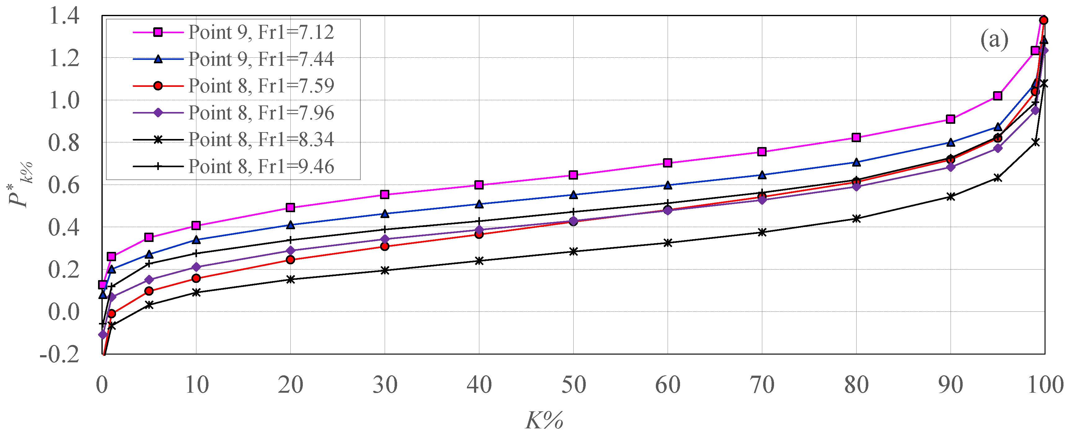
3.2. Cumulative Pressure Curves

From the pressure data with different probabilities (P*_k%), the cumulative pressure curves were provided for each pressure tap with different Froude numbers. Figure 6 presents the cumulative pressure curves for P*_k% related to the characteristic points of X*_σmax, X*_d, X*_r, and X*_j, respectively.

According to Figure 6, P*_k% values increase with increasing probability (k%). Minimum pressure data (P*_min) correspond to the lowest probabilities (P*_1%). On the contrary, maximum pressure data (P*_max) correspond to the highest probability (P*_99%). Accordingly, the maximum pressure fluctuations, and the negative pressures, are located at the positions near the spillway toe. Also, the minimum pressure fluctuations are located at the positions downstream of the hydraulic jump.

3.3. Proposition of New Relationships

Based on the results obtained, it was observed that the method proposed by Teixeira [26] could be optimized to be used for present data, or in similar conditions by using another relationship for the dimensionless standard deviation of pressure fluctuations (σ*_X). Thus, a new second-order fractional relationship (rational model), as a function of the dimensionless position along the stilling basin, is introduced.

$${\sigma }_X^{*}=\frac{a+b{X}^{*}}{1+c{X}^{*}+d{X}^{{*}^2}}0\le X^{*}\le 7$$

(15)

where a = 0.3414, b = 0.0299, c = −0.4264, and d = 0.0994. Figure 7 shows the corresponding scatter plot of σ*_X, and fitting of Equation (15), with a determination coefficient (R²) equal to 0.776.

In the present study, the values of N_k% with different non-exceedance probabilities are determined. Figure 8 shows the longitudinal distribution of the N_k% coefficient.

From the analysis of Figure 8, the constant values of the coefficient N_k% are developed along the jump, especially in the case of pressures with probabilities of 5%, 10%, 90%, and 95%. Therefore, depending on the probability, the values of the coefficient of N_k% indicate a single mean value for each probability. According to Wiest [42], there is no significant effect of the parameter of Fr₁, and the values of N_k% remain somewhat constant throughout the basin. A new second-order fractional relationship (rational model) can estimate the N_k% coefficient with a determination coefficient (R²) equal to 0.98.

$$N_{k\%}=\frac{a+bk}{1+ck+d{k}^2}$$

(16)

where a = −3.1347, b = 6.2140, c = 12.9495, and d = −13.0039, and k is the probability value (in decimal value). Figure 9 shows the mean values of the coefficient N_k% for each probabilities (k%), and the proposed relationship (Equation 16).

3.4. Comparison between Sample and Estimated Pressure Data

Figure 10 presents the distributions of P*_k% with probabilities of 1%, 5%, 10%, 90%, 95%, and 99%. Experimental data are presented as a function of X*, together with the corresponding estimates using Teixeira [26], also modified using Equation (15).

Accordingly, close to the spillway toe, pressure data with low and high probability, especially for P*_1% and P*_99%, have lower and higher values, with the maximum differences than P*_m. P*_1% data reach negative values down to −0.2, at the position X* ≈ 2, indicating regions with low pressures. To evaluate the performance of the experimental and the estimated values of σ*_X, some statistical performance criteria including determination coefficient (R²) [39], root mean squared error (RMSE) [39], mean absolute error (MAE) [39], Willmott’s index of agreement (WI) [43] are provided in

Table 4. Results of the statistical performance criteria for σ*_X.

Method	R2	RMSE	MAE	WI
Equation (15)	0.776	0.097	0.075	0.931
[26]	0.674	0.140	0.115	0.875

. As a result, the goodness of fit statistics for the estimation of σ*_X is confirmed.

For proper performance, RMSE and MAE should be close to zero; and R² and WI values should be close to the unit. According to Table 4, this relationship for σ*_X provides better estimation performance as compared against Teixeira [26]. The new relationship is given in Equation (15) presents somewhat better results for P*_90%, P*_95%, and P*_99% along the stilling basin.

4. Conclusions

In this study, extreme pressures beneath hydraulic jumps inside the USBR Type I stilling basin (smooth bed) downstream of an Ogee spillway, are investigated for different incident Froude numbers ranging from 7.12 to 9.46. In summary, several conclusions are provided as follows:

(1)

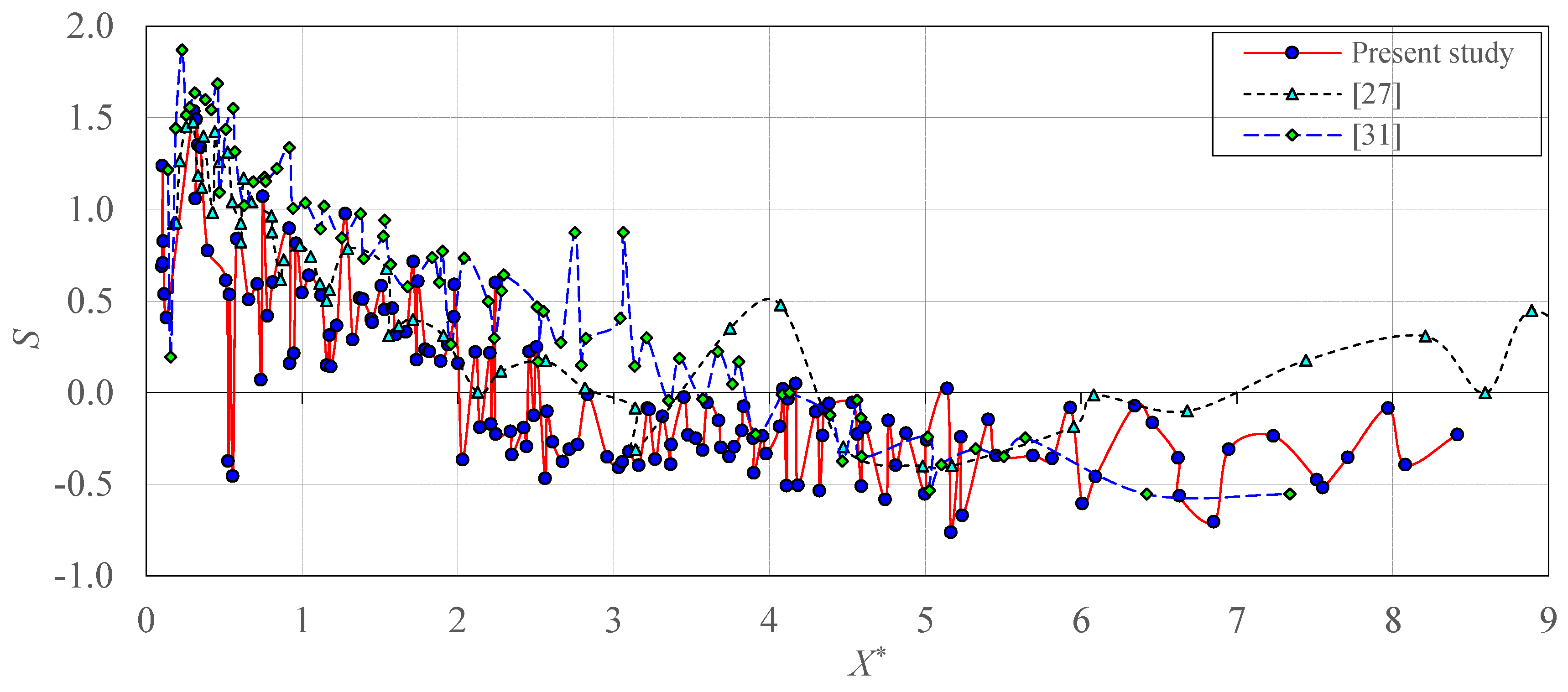
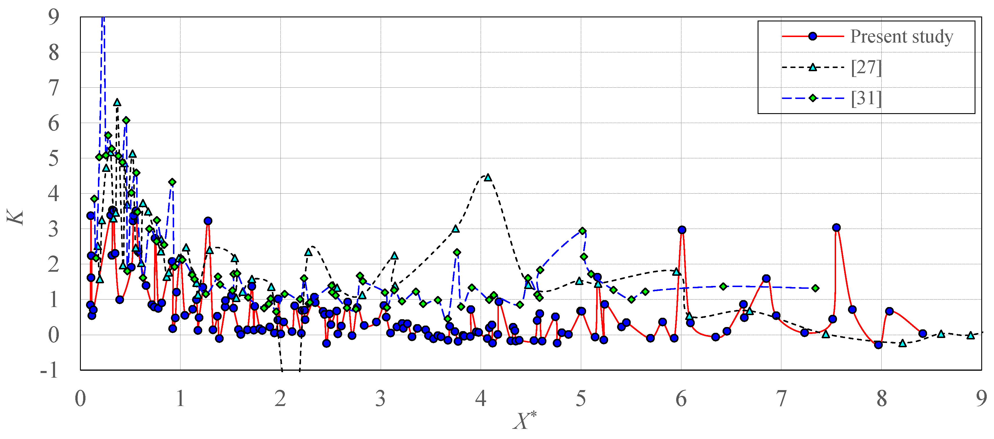
Sample skewness (S) and kurtosis (K) coefficients indicated that the pressure distribution along the hydraulic jumps does not follow a normal distribution. Some characteristic points are the maximum pressure fluctuations point (X*_σmax) with S_max; the flow detachment point (X*_d) with S ≈ 0; the roller endpoint (X*_r) with S_min; and the hydraulic jump endpoint (X*_j) with S ≈ 0.

(2)

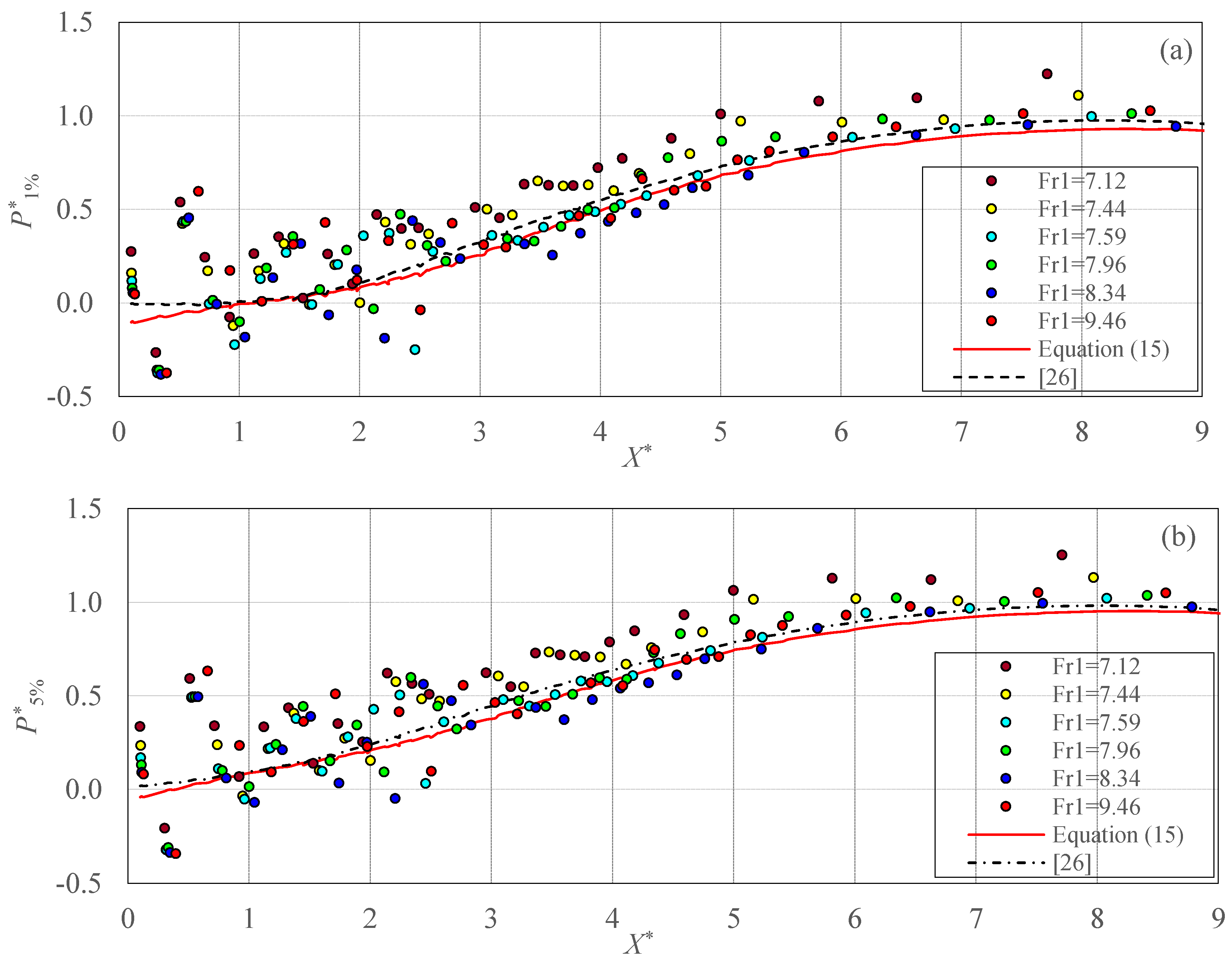
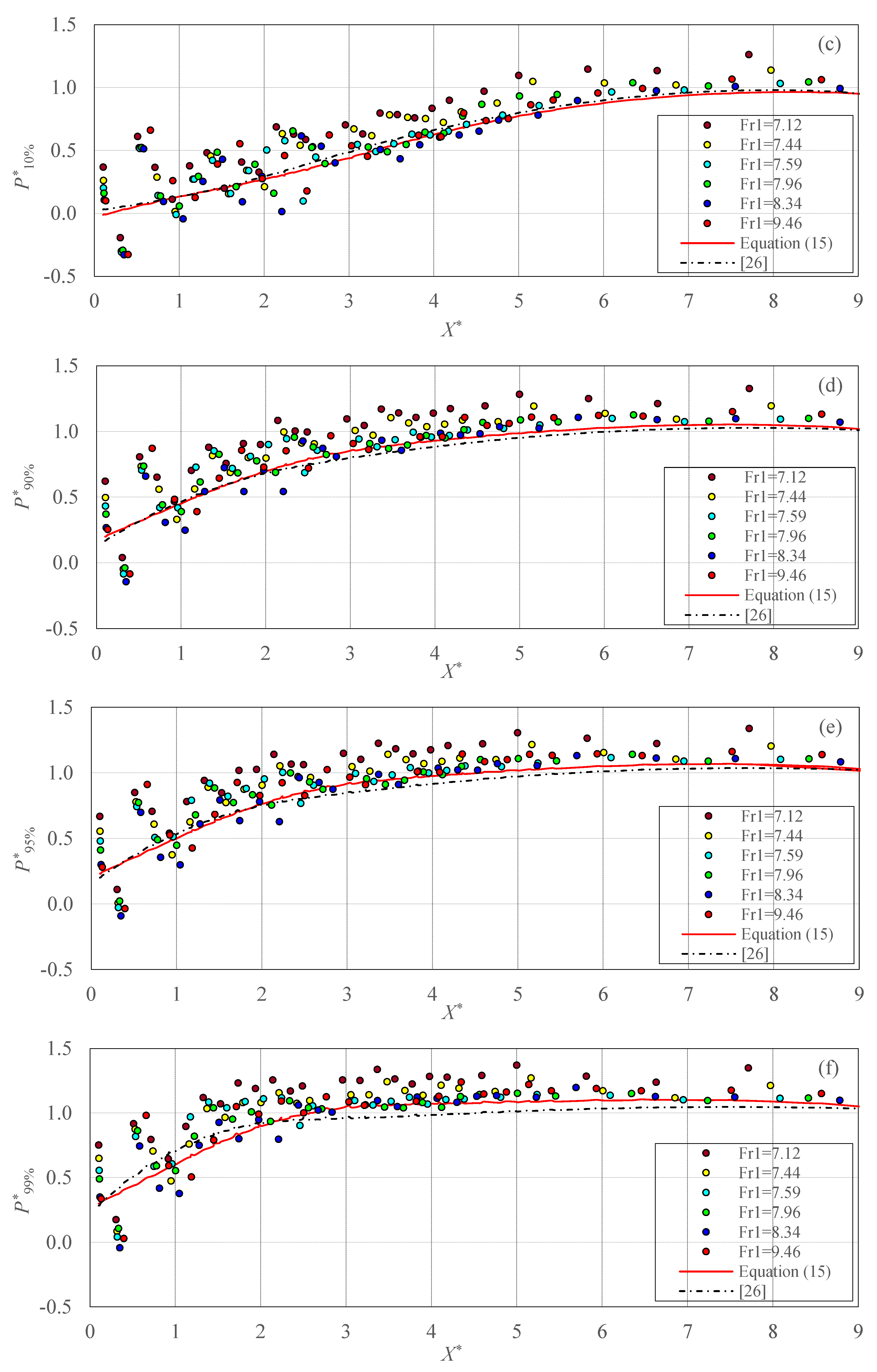
From the pressure data with different non-exceedance probabilities (P*_k%), the cumulative pressure curves are presented for P*_k% related to the characteristic points of X*_σmax, X*_d, X*_r, and X*_j, respectively. For the positions close to the spillway toe, pressures with low and high probability (P*_1% and P*_99%), have lower and higher values, with the maximum differences than P*_m. P*_1% data, reach negative values down to −0.2, at the position X* ≈ 2, indicating regions with low pressures.

(3)

From the analysis of the probability distribution of the sample data as collected by pressure transducers, pressures data of P*_k% can be determined.

(4)

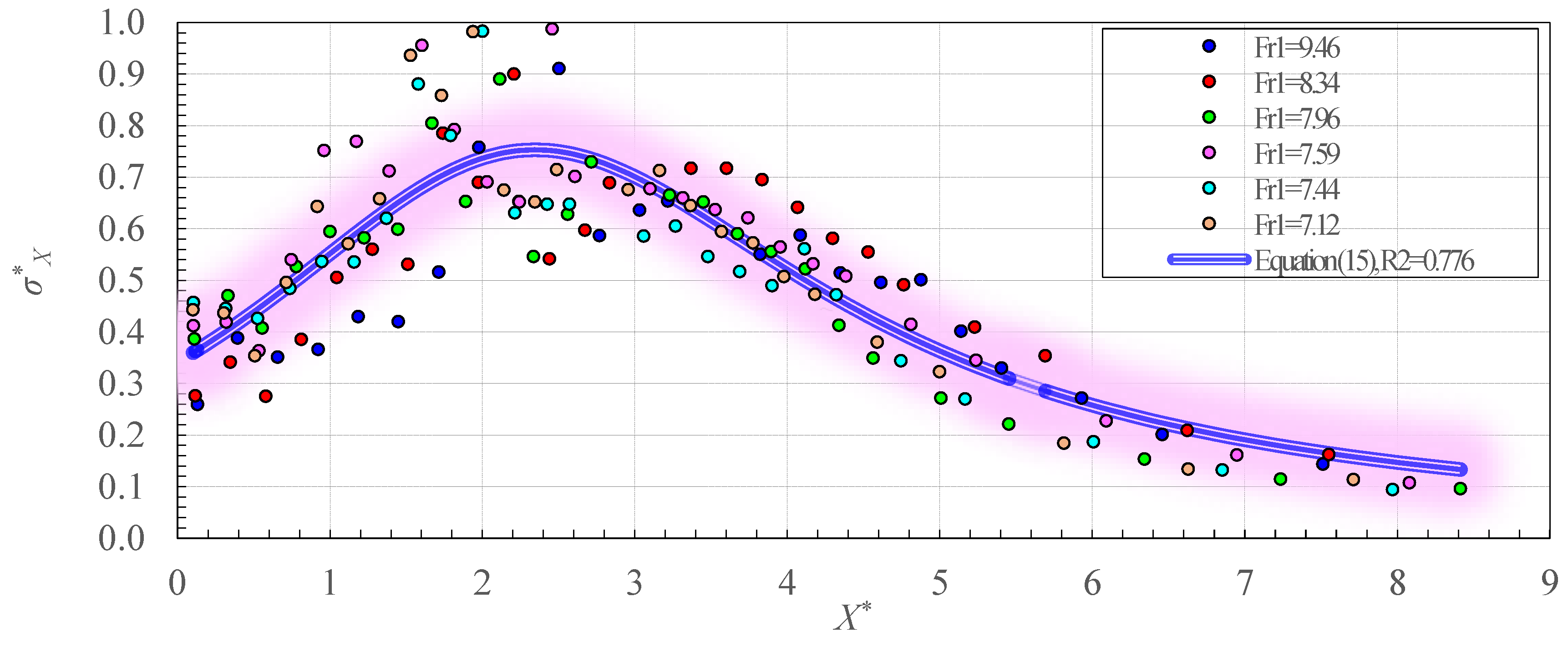
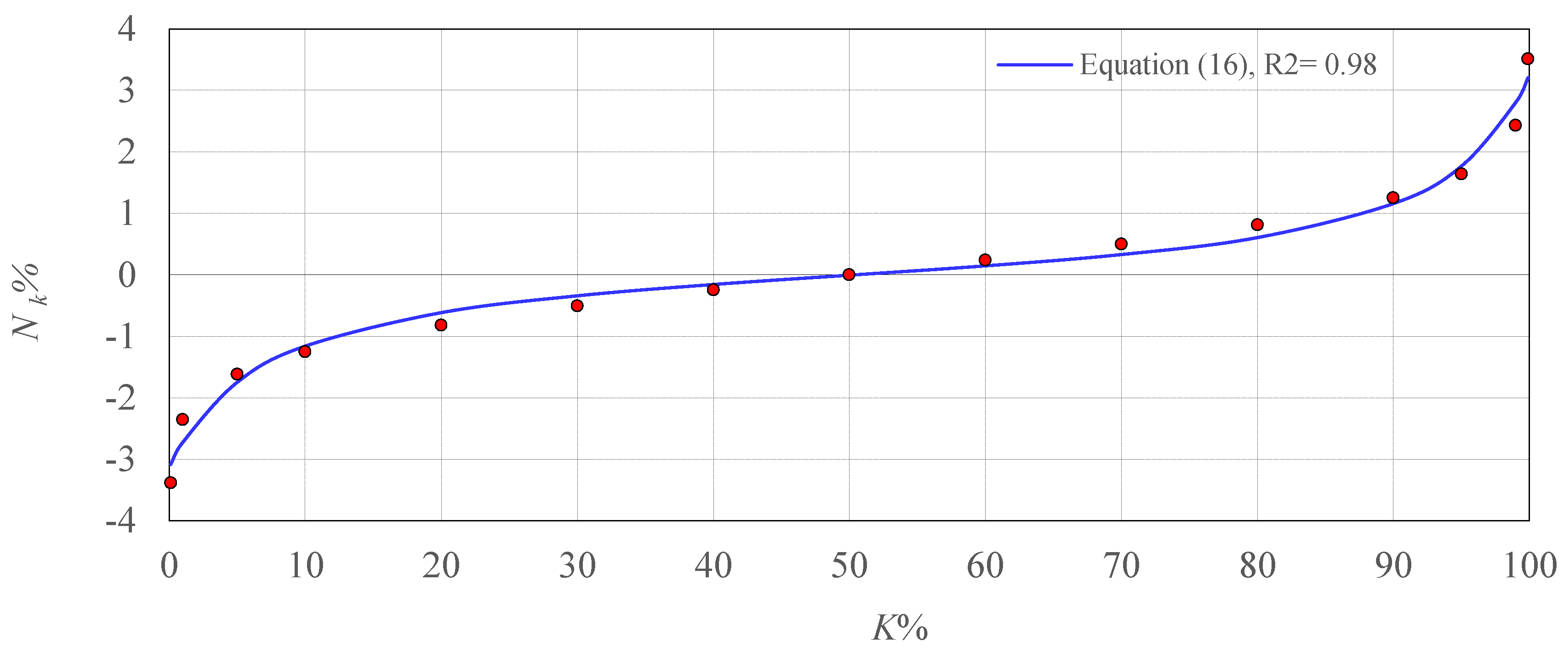
Based on the results obtained, it was observed that the method proposed by Teixeira [26] could be optimized to be used for present data, or in similar conditions by using another relationship for the dimensionless standard deviation of pressure fluctuations (σ*_X), and the statistical coefficient of the probability distribution (N_k%). Thus, a new second-order fractional relationship, as a function of the dimensionless position along the stilling basin (X*), is introduced for σ*_X. This relationship is valid for the dimensionless positions (X*) in the range of 0 to 8.4. To assess the accuracy of this relationship, some performance criteria are used. For the new proposed relationship (σ*_X) in this study, the values of R², RMSE, MAE, and WI were achieved 0.776, 0.097, 0.075, and 0.931, respectively. The constant values of N_k% are developed along the jump. Therefore, depending on the probability, the values of the N_k% coefficient indicate a single mean value for each probability. A new second-order fractional relationship was proposed to estimate the N_k% coefficient with R² = 0.98. The new relationships should be validated against sample data taken in similar conditions to our case study here.

(5)

The results contribute to enhancing the knowledge of the flow in a USBR Type I stilling basin that can be used to improve their design. This work only includes the case of free jumps. Future advancements will cover the behavior of submerged jumps with variable submergence degrees, resulting in modified pressure fields concerning those observed here for free jumps. As well, the efficiency of blocks and sills with different sizes may be investigated. A more extensive range of flow discharge will need to be explored. In the future, the more specific effort may be devoted to testing other possible distributions, fitting the observed pressure fields and their use in practice design. Also, velocity fields within the hydraulic jump may be investigated to define the turbulent components of flow fields.

References

- Valero, D.; Viti, N.; Gualtieri, C. Numerical simulation of hydraulic jumps. Part 1: Experimental data for modelling performance assessment. Water 2019, 11, 36. [Google Scholar] [CrossRef]
- Toso, J.W.; Bowers, C.E. Extreme pressures in hydraulic-jump stilling basins. J. Hydraul. Eng. 1988, 114, 829–843. [Google Scholar] [CrossRef]
- Khatsuria, R.M. Hydraulics of spillways and energy dissipators; Marcel Dekker: New York, NY, USA, 2005. [Google Scholar]
- Bukreev, V. Statistical characteristics of the pressure fluctuation in a hydraulic jump. J. Appl. Mech. Tech. Phys. 1966, 7, 97–99. [Google Scholar] [CrossRef]
- Locher, F.A. Some Characteristics of Pressure Fluctuations on Low-Ogee Crest Spillways Relevant to Flow-Induced Structural Vibrations; Iowa Institute of Hydraulic Research, The University of Iowa: Iowa City, IA, USA, 1971. [Google Scholar]
- Schiebe, F.R. The Stochastic Characteristics of Pressure Fluctuations on a Channel Bed due to The Macroturbulence in a Hydraulic Jump. Ph.D. Thesis, University of Minnesota, Twin Cities, MN, USA, 1971. [Google Scholar]
- Abdul Khader, M.; Elango, K. Turbulent pressure field beneath a hydraulic jump. J. Hydraul. Res. 1974, 12, 469–489. [Google Scholar] [CrossRef]
- Lopardo, R.; Vernet, G.; Ronaldo, R. Correlation of instantaneous pressures induced by a free and stable hydraulic jump. In Proceedings of the XI Latin American Congress of Hydraulics IAHR, Ezeiza, Argentina, 3 April 1984; pp. 23–34. (In Spanish). [Google Scholar]
- Lopardo, R.A. Methodology for estimating instantaneous pressures in dissipation basins. In Proceedings of the Annals of the University of Chile, Santiago, Chile, 20 June 1985; pp. 437–455. (In Spanish). [Google Scholar]
- Farhoudi, J.; Narayanan, R. Force on slab beneath hydraulic jump. J. Hydraul. Eng. 1991, 117, 64–82. [Google Scholar] [CrossRef]
- Fiorotto, V.; Rinaldo, A. Turbulent pressure fluctuations under hydraulic jumps. J. Hydraul. Res. 1992, 30, 499–520. [Google Scholar] [CrossRef]
- Fiorotto, V.; Rinaldo, A. Fluctuating uplift and lining design in spillway stilling basins. J. Hydraul. Eng. 1992, 118, 578–596. [Google Scholar] [CrossRef]
- Armenio, V.; Toscano, P.; Fiorotto, V. On the effects of a negative step in pressure fluctuations at the bottom of a hydraulic jump. J. Hydraul. Res. 2000, 38, 359–368. [Google Scholar] [CrossRef]
- Yan, Z.-M.; Zhou, C.-T.; Lu, S.-Q. Pressure fluctuations beneath spatial hydraulic jumps. J. Hydrodyn. 2006, 18, 723–726. [Google Scholar] [CrossRef]
- Onitsuka, K.; Akiyama, J.; Shige-Eda, M.; Ozeki, H.; Gotoh, S.; Shiraishi, T. Relationship between pressure fluctuations on the bed wall and free surface fluctuations in weak hydraulic jump. In New Trends in Fluid Mechanics Research—Proceedings of the Fifth International Conference on Fluid Mechanics, Shanghai, China, 15–19 August 2007; pp. 300–303. [Google Scholar]
- Lian, J.; Wang, J.; Gu, J. Similarity law of fluctuating pressure spectrum beneath hydraulic jump. Chin. Sci. Bull. 2008, 53, 2230–2238. [Google Scholar] [CrossRef]
- Lopardo, R.A.; Romagnoli, M. Pressure and velocity fluctuations in stilling basins. In Advances in Water Resources and Hydraulic Engineering; Springer: Berlin/Heidelberg, Germany, 2009; pp. 2093–2098. [Google Scholar]
- Lopardo, R.A. Extreme velocity fluctuations below free hydraulic jumps. J. Eng. 2013, 2013, 1–5. [Google Scholar] [CrossRef][Green Version]
- Wang, H.; Murzyn, F.; Chanson, H. Total pressure fluctuations and two-phase flow turbulence in hydraulic jumps. Exp. Fluids 2014, 55, 1847. [Google Scholar] [CrossRef]
- Fiorotto, V.; Barjastehmaleki, S.; Caroni, E. Stability analysis of plunge pool linings. J. Hydraul. Eng. 2016, 142, 1–11. [Google Scholar] [CrossRef]
- Barjastehmaleki, S.; Fiorotto, V.; Caroni, E. Spillway stilling basins lining design via Taylor hypothesis. J. Hydraul. Eng. 2016, 142, 1–11. [Google Scholar] [CrossRef]
- Barjastehmaleki, S.; Fiorotto, V.; Caroni, E. Design of stilling basin linings with sealed and unsealed joints. J. Hydraul. Eng. 2016, 142, 1–10. [Google Scholar] [CrossRef]
- Gu, S.; Bo, F.; Luo, M.; Kazemi, E.; Zhang, Y.; Wei, J. SPH simulation of hydraulic jump on corrugated riverbeds. Appl. Sci. 2019, 9, 436. [Google Scholar] [CrossRef]
- Güven, A.; Günal, M.; Cevik, A. Prediction of pressure fluctuations on sloping stilling basins. Can. J. Civ. Eng. 2006, 33, 1379–1388. [Google Scholar] [CrossRef]
- Hager, W.H. B-jump in sloping channel. J. Hydraul. Res. 1988, 26, 539–558. [Google Scholar] [CrossRef]
- Teixeira, E.D. Scale effect on estimating extreme pressure values on the bed of the hydraulic dissipation basins. Ph.D. Thesis, Hydraulic Reseach Institute, Federal University of Rio Grande do Sul, Porto Alegre, Brazil, 2008. (In Portuguese). [Google Scholar]
- Teixeira, E.D.; Neto, E.F.T.; Endres, L.A.M.; Marques, M.G. Analysis of pressure fluctuations near the bed in hydraulic jump dissipation basins. In Proceedings of the Brazilian Dam Committee, XXV Large Dams National Seminar, Salvador, Brazil, 12–15 October 2003; pp. 188–198. (In Portuguese). [Google Scholar]
- Souza, P.E.d.A.; Marques, M.G.; Neto, E.F.T.; Teixeira, E.D. Pressure fluctuation in a low-drop and low Froude numbers of hydraulic jump downstream of a spillway. In Proceedings of the Brazilian Dam Committee, XXX - Large Dams National Seminar, Foz do Iguaçu, Brazil, 11–13 May 2015; pp. 1–14. (In Portuguese). [Google Scholar]
- Prá, M.D.; Teixeira, E.D.; Marques, M.G.; Priebe, P.d.S. Evaluation of Pressure Fluctuation in Hydraulic Jump by Dissociation of Hydraulic Forces. Braz. J. Water Resour. (Rbrh) 2016, 21, 221–231. (In Portuguese) [Google Scholar]
- Novakoski, C.K.; Hampe, R.F.; Conterato, E.; Marques, M.G.; Teixeira, E.D. Longitudinal distribution of extreme pressures in a hydraulic jump downstream of a stepped spillway. Braz. J. Water Resour. (Rbrh) 2017, 22, e42. [Google Scholar] [CrossRef][Green Version]
- Marques, M.G.; Drapeau, J.; Verrette, J.-L. Pressure fluctuation coefficient in a hydraulic jump. Braz. J. Water Resour. (Rbrh) 1997, 2, 45–52. (In Portuguese) [Google Scholar]
- Farhoudi, J.; Sadat-Helbar, S.; Aziz, N.I. Pressure fluctuation around chute blocks of SAF stilling basins. J. Agric. Sci. Technol. 2010, 12, 203–212. [Google Scholar]
- Padulano, R.; Fecarotta, O.; Del Giudice, G.; Carravetta, A. Hydraulic design of a USBR Type II stilling basin. J. Irrig. Drain. Eng. 2017, 143, 04017001. [Google Scholar] [CrossRef]
- USBR. Spillways. In Design of small dams, 3rd ed.; US Department of the Interior, Bureau of Reclamation: Washington, DC, USA, 1987; pp. 339–437. [Google Scholar]
- Chanson, H.; Carvalho, R. Hydraulic jumps and stilling basins. In Energy Dissipation in Hydraulic Structures; Chanson; CRC Press: Leiden, The Netherlands, 2015; pp. 65–104. [Google Scholar]
- Rajaratnam, N. Hydraulic jumps. In Advances in Hydroscience; Elsevier: Edmonton, Canada, 1967; Volume 4, pp. 197–280. [Google Scholar]
- Peterka, A.J. Hydraulic Design of Stilling Basins and Energy Dissipators, 8th ed.; U.S. Dept. of the Interior, Bureau of Reclamation: Denver, CO, USA, 1984.
- Chaudhry, M.H. Open-Channel Flow, 2nd ed.; Springer Science & Business Media: New York, NY, USA, 2008. [Google Scholar]
- Bennett, N.D.; Croke, B.F.; Guariso, G.; Guillaume, J.H.; Hamilton, S.H.; Jakeman, A.J.; Marsili-Libelli, S.; Newham, L.T.; Norton, J.P.; Perrin, C. Characterising performance of environmental models. Environ. Model. Softw. 2013, 40, 1–20. [Google Scholar] [CrossRef]
- Bono, R.; Arnau, J.; Alarcón, R.; Blanca, M.J. Bias, precision, and accuracy of skewness and kurtosis estimators for frequently used continuous distributions. Symmetry 2020, 12, 19. [Google Scholar] [CrossRef]
- Sharma, C.; Ojha, C. Statistical parameters of hydrometeorological variables: standard deviation, SNR, skewness and kurtosis. In Advances in Water Resources Engineering and Management; Springer Singapore: Singapore, 2020; Volume 39, pp. 59–70. [Google Scholar]
- Wiest, R.A. Evaluation of the pressure field in hydraulic jump formed downstream of a spillway with different submergence degrees. Master’ Thesis, Hydraulic Reseach Institute, Federal University of Rio Grande do Sul, Porto Alegre, Brazil, 2008. (In Portuguese). [Google Scholar]
- Willmott, C.J.; Robeson, S.M.; Matsuura, K. A refined index of model performance. Int. J. Climatol. 2012, 32, 2088–2094. [Google Scholar] [CrossRef]