Kinematics in Biology: Symbolic Dynamics Approach


Department of Mathematics, CIMA, University of Évora, 7000 Évora, Portugal
Mathematics 2020, 8(3), 339; https://doi.org/10.3390/math8030339
Submission received: 28 January 2020
/
Revised: 26 February 2020
/
Accepted: 28 February 2020
/
Published: 4 March 2020
(This article belongs to the Special Issue Mathematical Biology: Modeling, Analysis, and Simulations)
Abstract
:Motion in biology is studied through a descriptive geometrical method. We consider a deterministic discrete dynamical system used to simulate and classify a variety of types of movements which can be seen as templates and building blocks of more complex trajectories. The dynamical system is determined by the iteration of a bimodal interval map dependent on two parameters, up to scaling, generalizing a previous work. The characterization of the trajectories uses the classifying tools from symbolic dynamics—kneading sequences, topological entropy and growth number. We consider also the isentropic trajectories, trajectories with constant topological entropy, which are related with the possible existence of a constant drift. We introduce the concepts of pure and mixed bimodal trajectories which give much more flexibility to the model, maintaining it simple. We discuss several procedures that may allow the use of the model to characterize empirical data.
1. Introduction
Motion was one of the first topics considered in science. In fact, it was precisely from the study of motion that was developed modern science. Before the discovery of the causes of motion, with the development of dynamics and the concept of force with Newton, was important the comprehension of the geometry of the trajectories—kinematics—with Kepler and Galileu. In biology, with the enormous variety of phenomena and concepts, it is easy to be overwhelmed with information and interrelated data. It is difficult to simplify as in physics. There are too many parts with non-negligible interactions, characteristics of what is now called complex system. It is natural to develop stochastic methods, as an extension of statistical mechanics methods, to obtain statistical regularities and from it to make predictions about the long term behavior of the biological systems. It is necessary to give some apriori assumptions in order to chose the appropriate distributions, or to consider a completely empirical based approach in which machine learning with Bayesian methods, or others, can be employed without an explicit stochastic model.
On the other hand, the natural quasi-stochastic behavior of many chaotic deterministic systems, despite its eventually simple definition, may present an opportunity to explore new conceptual approaches which are in fact part of the old dynamics.
Animal movement and dispersal is an essential aspect in a variety of phenomena considered in biology, ecology and biogeography. Improvements on the subject depends on appropriate mathematical methods and have impact on the study of spreading of diseases, population dynamics, animal locomotion, and many other areas. The study of complex individual movement has attracted much attention since Mandelbrot observed that certain types of trajectories exhibit scale invariance and fractal properties. These properties are reflected in the type of distributions of the movement lengths, for example, inverse power law-like tail. Much work in the literature on the subject follows this perspective and it has been applied to different animal movements, from bird flight, insect movement and human movement to large size animals such as whales and other.
The methods used vary, ranging from pure stochastic, see for example the survey [1], machine learning or mechanistic approaches. An important reference in this last direction of study is Reference [2], where a conceptual framework for movement in ecology is proposed. Their approach is general and includes certain components which determine the movement path. Three of these components regard the individual and are: internal state, motion capacity and navigation capacity. A fourth component, corresponding to the external factors, represents aspects of the abiotic and biotic environment which affect the movement.
In Reference [3], the authors review literature on the agent based modeling approach allowing to incorporate in simulations characteristics of animal behavior and the interaction with different environments. Other methods are introduced and developed in References [4,5,6]. For example, state space models appropriate to deal with biological and statistical features of satellite tracking data and different methodologies of collecting data using statistically robust methods. The state-space framework considers the internal state of the animal as a possible state variable which influence the displacement, therefore allowing the transition between behavior states or modes, within the model. This is important for the observed type of trajectory, since the animal may be migrating, searching for water, foraging, exploring, and these types of behavior produce distinct types of trajectories.
In Reference [7], the authors refer to alternative methods for modeling animal trajectories with hidden Markov models, where the modeling is based on existing non-observable states which are governed by some probability distributions, for example, Markov chains. The authors discuss these methods comparing them with the state-space model approach. The computational tractability and mathematical simplicity are stressed as main advantages of the referred methods, and the authors apply the models to changing behavior of the animals and to multiple animal movement description.
Until recently there remains some academic debate with respect to the stochastic nature of animal movement and the appropriate length probability distribution in the characterization of animal movements, in particular, regarding the importance or not of the Levy walk type. See, for example References [8,9].
The objective of the present paper is to develop a model, introduced in Reference [10], which simulate and classify different types of trajectories using a very simple iterated map of the interval—a cubic map , depending on two parameters . The map produce the displacements in each Cartesian coordinate through iteration. We consider that the produced trajectories are identified as typical paths of certain animals which at some extent are isolated, with stable behavior, or exposed to a constant external influence. The characteristics, patterns or irregularities of the trajectory are codified in the symbolic description of the orbits of , through the alphabet , corresponding to the partition of monotonicity of . The iterated map is seen as a descriptive classifying tool, establishing, through symbolic dynamics, a dictionary for trajectories. The main classifying tool is the kneading invariant, , of the map , which is composed by two symbolic sequences. These sequences correspond to the symbolic itineraries of the critical points which are attractors for the dynamics. Therefore, this pair of orbits determine the behavior of every orbit in the system. Roughly speaking, we associate to a particular patch, or piece of trajectory, a symbolic sequence or a class of symbolic sequences. Thus, the study of the possible trajectories and its properties can be made enumerating symbolic sequences satisfying certain combinatorial constrains. On the other hand, using ergodic theory for symbolic dynamics and for iterated maps of the interval we may derive the probability distributions which are, in this case, a consequence of the model. The model introduced in Reference [10] depends on a real number b which parametrizes the complexity of the trajectories in the isolated case, since the topological entropy of the system depends monotonically on b. Here, we include a new parameter d which serves to describe the existence of persistent drift affecting globally the movement and models the effect of some constant external influence. This new parameter implies the use of the topological invariant introduced by Sousa Ramos and his collaborators in Reference [11]. This invariant classifies and distinguishes dynamics with the same topological entropy, that is, allows the characterization of isentropic trajectories—which are only possible with the introduction of an external influence provoking the constant drift. Typically, low topological entropy values give direct motion, with very few changes in direction, or regular changes in direction. On the other hand, high topological entropy gives large variation on direction and many different possible patterns of changing direction.
The model is scale independent, since it can be applied directly from the microscopic scale to the scale of the largest animal in earth. This is obtained through the choice of an external scale parameter , which is related to the largest linear step possible for the particular animal.
Differently from the stochastic approaches, there is no fixed model of probability distribution. In fact, there are many families of probability distributions, depending only on the chosen parameters or on the kneading invariant, arising from the long term dynamics of .
Although the model is deterministic, particular observed animal trajectories are not necessarily reproduced in an exact manner. From the pattern of an observed trajectory, the number of consecutive steps where the direction is approximately maintained are identified, as the changes in direction and the consecutive steps of changing direction. Then, it is possible to produce a sequence in the referred alphabet , associated with the observed trajectory. Next, it is possible to determine, at least, a class of kneading sequences which turns the observed sequence into admissible with respect to the iterated map. In this case, the approximate values for the topological entropy and other invariants can be computed, obtaining a characterization of the system which produces similar trajectories, as the given one. This process still needs some details to be completed. It will be considered later, in a paper dedicated exclusively on dealing with empirical data and experimental procedure to find the best way to fit the bimodal trajectories on empirical trajectories.
The model, here discussed, is of interest at theoretical level taking into account the range and variety of behaviors and trajectories for the simple deterministic system, many theoretical questions may be posed. It is of numerical and simulation interest since it can be seen as a pseudo-random number generator suitable for trajectory analysis, considering the chaotic behavior for certain values of the parameters. We outline that for the mean square displacement of the trajectories, we obtain diffusive type of behavior, with exponents close to , sub-diffusive, with exponents less than and superdiffusive with exponents between and 1. See the dictionary in Section 6.
We expect that using this method to describe the motion of an animal it is possible the development of a more complete model, maintaining its simplicity, including interactions with the environment and with other animals. This can be pursued allowing the dependence of the parameters on the position or on the displacement, obtaining an larger dynamical system or a non-autonomous discrete dynamical system.
The paper is organized as follows: In Section 2 we review general assumptions which support certain aspects of the model. In Section 3 we review the symbolic dynamics techniques used for bimodal maps, namely its classification, and the definition of the topological Markov chain in the periodic and pre-periodic case. In the Section 4 we discuss the notion of isentropic dynamics and classify the behaviors with only one attractor. In Section 5 we introduce the model and discuss its interpretation and direct consequences. Moreover, we discuss certain adaptations to make the model usable with empirical data. In the Section 6 we present numerical results for a sample of the dictionary, showing the relation between parameters, symbolic sequences and the trajectories behavior.
2. Kinematics of Isolated Animal
Kinematics, in physics, study the motion of a particle or a body, from a geometrical point of view. There are intrinsic characteristics of the object which may have to be considered such as mass or the electrical charge. If there is no force present we obtain uniform movement with constant velocity and zero acceleration. With a constant force, for example, the gravitational force, we may have, depending on the initial conditions, a straight line, a parabola, an ellipse or hyperbola. With a time dependent force we pass from kinematics to dynamics, we have to introduce an interaction between the objects and have to consider the Newton laws of motion.
With a similar reasoning we may consider the kinematics of the isolated animal, as proposed in Reference [10]. The concept of isolated animal is comparable to the notion of isolated body in physics. An isolated system does not exist in real world, however, is an essential abstraction to conceptual development, hypothesis formulation and for the design of experimental apparatus which may indicate new hypothesis, infirm or confirm stated ones.
In the context of the animal movement study, taking an observational point of view, we may conceive a systematic study in which different kinds of species are considered. The study of movement of the considered animals can be made in controlled environments, maintaining constant every abiotic parameters, such as temperature, light, humidity, type of underlying material/terrain and so on. The experimental apparatus can be progressively improved eliminating possible causes of gradients, maintaining the environment the most homogeneous possible. For each specie several individuals may be considered and tested, and several runs or tracks are observed for each individual. We may observe that the trajectories are irregular and different even for the same animal—it is not common an animal repeating exactly the same trajectory, unless there is an external influence causing this repetition. However, it is natural to suspect that there are some patterns, eventually common to many different species and eventually depending on the internal state of the animal—hungry, tired, exhaustion, other.
A natural question is, then, the following—what is a typical motion of an animal in isolated or strongly controlled conditions?
It is interesting to consider this question either experimentally or theoretically. Taking these observations into account let us see how far we can go, theoretically, with the simplifying assumptions given next:
- (1)
- Metabolism or internal dynamics as the only cause of motion: Isolated animal.
- (2)
- Motion is composed of discrete linear steps.
- (3)
- There is a maximal displacement, in one step, which is a consequence of the finite size of the animal and the finite energy at disposal.
- (4)
- Any step depends on the previous step taken: Markov hypothesis.
These four assumptions, (1), (2), (3), (4), allow the use of an iterated map to produce the steps at discrete time instants, t, which can be scaled so that .
Next, the following assumptions determine further the structure of the model and the specific families of iterated maps we may consider to produce the trajectory.
- (5)
- Differentiability/Continuity: close steps give origin to close steps.
- (6)
- Isotropy: there is no preferential direction for the motion.
- (7)
- One parameter characterizing the iterated process so that there exist for some values of the parameter, at least, one chaotic attractor.
Some consideration can be made:
- (a)
- From the assumption (1) the movement of an animal in isolation depends on its internal state or metabolism. This does not mean that the motion is simple. Moreover, the internal state of the animal may change with time and with the energy spent in the motion. Therefore, next to these basic assumptions we have to consider, theoretically and empirically, the dependence of patterns of motion according to the behavior associated with the internal states of the animal. This issue will be considered in future work in detail. Here, we simple aim to describe geometrically short time patches of trajectories, seen as templates or archetype movements, in which the animal behavior is ideally stable. An implicit assumption here is that we have a correspondence between animal behavior and the parameters determining the geometry trajectory.
- (b)
- If eventually, the empirical data shows that the trajectories are not well described by linear steps, then the assumption (2) can be read as the trajectories following approximately the linear step, that is, are contained in a rectangle of wide which contains the linear step. This point is discussed in Section 5.
- (c)
- There is no special reason for the assumption (5). The alternative would need eventually a cause or an explanation for the existing discontinuity or point without derivative. We could assume that there are discontinuity points (in a finite number) for some reason. Eventually, empirical data may require this adjustment. In future work we plan to deal with this issue.
- (d)
- The existence of a chaotic attractor assumed in (7) allows the simulation of the animal movement with a deterministic model. The variability of the trajectories is codified in the initial condition for the chaotic system and in its parameters. In a certain sense, due to the chaotic nature of the model we can see it as a pseudo random number generator which is adequate to produce typical trajectories with varied geometrical and statistical properties. We can chose initial conditions randomly or if we pretend a particular trajectory, with prescribed characteristics, we can obtain it, since the process is deterministic.
- (e)
- Different types of coordinates can be considered, using the above assumptions. We have tested polar coordinates and coupled Cartesian coordinates. However, in the present paper, as in Reference [10], we focus on Cartesian uncoupled coordinates. A general framework using matricial iteration is very promising and will be used in forthcoming paper. There are several reasons to focus, on a first approach, on the very simple iterated maps with uncoupled Cartesian coordinates: (1) its symbolic dynamics is well known, (2) the two or three dimensional trajectories can be reduced to one dimensional dynamics (3) the complexity of trajectories obtained is sufficiently interesting and varied to be analyzed.
- (f)
- Since we are considering isolated animal if there is symmetry breaking this means that the animal has in its internal processes a preference to some direction. For example, the possibility of detecting magnetic field, light, heat or other phenomena. This point is very interesting for certain classes of animals, however in this case we do not have isolation.
These assumptions and considerations led, in Reference [10], to a symmetrical bimodal map as the simplest model to produce the isotropic displacements in each Cartesian coordinate, and which fulfills the above assumptions. Among the bimodal maps, a particular bimodal family was chosen, simple from the analytical and numerically point of view: the cubic family, , of symmetric surjective bimodal maps on the interval ,
3. Bimodal Maps
General bimodal maps, which are continuous maps with two critical points, are characterized by two parameters, up to topological conjugacy. In an equivalent way, they are characterized by two symbolic sequences called kneading sequences, corresponding to the symbolic itineraries of the critical points, see Reference [12] for details, and below for the definition. Assuming the conditions referred in the previous section: isotropic motion, rest position as a possible solution and the simplest situation in which we have one attractor or two symmetrical attractors, we arrive to a family of interval maps which are symmetric and bimodal, that is, differentiable with two critical points, and . This family is topologically equivalent, through conjugation of an interval homeomorphism, to a one-parameter family of the interval . The simplest case possible, in terms of analytical expression, is a symmetric cubic map
If we consider a possible symmetry breaking of isotropy, consequence on some external effect on the animal, this leads directly to a general bimodal map with two parameters.
3.1. Symbolic Dynamics for Bimodal Maps
Consider the general family, , derived from the symmetric surjective bimodal maps introduced above:
Note that when we recover the symmetric family . This particular parametrization is surjective on , for the parameters in some region to be defined below.
We consider the discrete dynamical system, referred in the introduction, as the pair and the orbit of a point is the set
obtained under iteration of . The critical points of are denoted by
where denotes the absolute value of b. Therefore, independently on the sign of b we have .
Let us introduce the region of the parameters where the dynamics on is well defined. Well defined means the orbits of the critical points are contained in , independently of the critical points are in fact inside . This leads to the conditions , , and to the explicit condition on the parameters:
since the images of the critical points, the critical values, are equal to . However, this includes regions with very simple dynamical behavior and without much to study dynamically. It is natural to impose additional conditions, namely the condition that the two critical points are themselves contained in the interval . This gives us , and in terms of the parameters
In Figure 1 we represent the region delimited by the conditions (1) and the conditions (2). Moreover, we include the graphics of the bimodal for the points indicated in the boundary of the regions discriminated. The relevant dynamical parameter region is
where is distinguishing the signs of the parameters . The region has not the signs of the parameters discriminated since its behavior is very simple and direct. The regions which compose correspond to the cases in which both the critical points are in the interval and its orbits contained also in . The chaotic behavior region is contained in . Note that the region is disconnected according to the sign of b, that is, its connected components are and .
Let denote the intervals where is contractive. They are intervals centered in the critical points . Every point starting in will be attracted to the orbit of the critical point . Almost every point, with respect to Lebesgue measure, in the interval , under iteration, will reach one of , in finite time. Therefore, almost every orbit is strongly conditioned by the orbits of the critical points. If the critical point is periodic then almost every point in the interval is eventually attracted to that periodic orbit. If the critical orbit is aperiodic then almost every point in the interval is eventually attracted to it and we have chaotic motion. However, if the topological entropy is positive the case of periodic critical point has appreciable complex behavior. On one hand, the transient behavior changes significantly, changing the parameters . On the other hand, there is an infinite number of periodic orbits, unstable, of any period, which coexist with the given attractive periodic orbit.
The topological entropy measures the chaotic behavior of a discrete dynamical system. Roughly speaking, positive topological entropy is usually associated with chaotic behavior, that is, sensitivity dependence to initial conditions, existence of a transitive orbit, coexistence of infinite repulsive periodic points. The topological entropy is a topological invariant for and can be computed as the logarithm of the growth number of . The growth number is the growth rate of the number of periodic orbits with increasing size k. On the other hand, in the Markov case, for which there is a Markov partition of the interval and a transition matrix associated with , the growth number can be calculated as the Perron eigenvalue of , see References [11,13], or below. In general, not necessarily Markov, the growth number can be computed as a zero of the kneading determinant, in the context of the kneading theory, see References [12,14].
To classify every type of behavior and to know exactly what type of orbits coexist, given , it is very efficient the use of combinatorial methods, namely symbolic dynamics, in which numerical orbits are represented by symbolic sequences. In what follows we give the notions necessary to use symbolic dynamics. For more details, on symbolic dynamics of bimodal maps, we refer to References [12,13,15,16].
The address of , with respect to , is defined by
If there is no possible ambiguity we drop the index in the address map, that is, . The itinerary of a point x, which collects the addresses of the points in the orbit of x, is defined by
and allows the correspondence of orbits, under iteration of , with symbolic one-sided sequences in the alphabet or , if we consider the orbits of the critical points. The space of one-sided sequences is denoted by or . A symbolic sequence is admissible, with respect to , if there is an initial condition so that . Note that depending on the space of admissible sequences, , can vary significantly.
The kneading invariant of is defined by
where and are the itineraries of the critical points and called kneading sequences.
In the symmetric case, , it is useful the notation , , , , , to express the symmetry of the admissible sequences. In particular, for any we have . In general, there are two distinct critical orbits , in this case necessarily, (two symmetrical atractors). Nevertheless, we may have one critical orbit, that is, the two critical points belong to the same orbit (one atractor), and in this case the kneading sequences must be periodic and , where t is the period.
The iteration of corresponds to the shift map on the symbolic space sequences, that is, we have a semi-conjugation
where
For different values of different types of sequences occur. When considering the alphabet some care is needed since the symbols are special. They represent points and the symbols represent intervals. To the symbol only follows the sequence , to the symbol only follows the sequence , and no other possibility. On the contrary to the symbols L, M, R, which can be followed by any other symbol, depending on the parameters . Therefore, the combinatorial diversity of sequences can be enormous.
To determine exactly which sequences occur as itineraries in the set of all possible sequences, , it is necessary to introduce an order relation in the set of sequences. First, we define the parity or sign function: the bimodal sign function is defined by
with
for , and
Consider the set ordered by
The induced order relation in the set of one-sided sequences is defined as follows. Consider two sequences and of . There is a number such that for . Then
if and only if
or
It can be easily seen that the symbolic order structure is compatible with the order in the real line. In fact, for , if and only if .
Let us characterize the orbits and symbolic sequences which are not critical, that is, does not have the symbol . Recall that a sequence is called admissible, with respect to or , if there is so that .
The combinatorial characterization for the admissible sequences is the following: A sequence is admissible if and only if and or and .
Let us now characterize the orbits and symbolic sequences which are kneading sequences: periodic if , pre-periodic if or aperiodic if . In every case .
In the following sentences, Q is in one of the previous three types:
A sequence Q is a maximal (resp. minimal) kneading sequence if and only if (resp. ), for every .
Let be an admissible periodic sequence. Let denote the point x in the interval satisfying . If there is no ambiguity we write , to simplify notation.
3.2. Topological Markov Chain
Let us consider the case of periodic and pre-periodic critical orbits. In this two situations there is a Markov partition of the interval , with respect to the iteration of . The Markov partition is obtained directly from the orbits of the critical points, and . From the periodicity, or pre-periodicity, there is a least natural number so that
that is, we obtain an invariant set of points. In this case, the set constitute precisely the set of boundary points of the Markov partition for . Each interval of the partition is associated to a finite word in the alphabet and to a Markov state. The kneading sequences are necessarily periodic or pre-periodic, that is, in the form
or
for some natural numbers .
Recall from Reference [10] that in the symmetric case the periodic and pre-periodic kneading sequences, are in the form
or
In the case are periodic or pre-periodic, with period , , and transient lengths , as in (4), the Markov partition and the transition matrix induced by can be explicitly determined from the symbolic sequences. We give the explicit construction here for the pre-periodic case considering that the periodic case is a particular situation with . The Markov partition is determined precisely by the successive shifts of the kneading sequences and ordered by ≺. Let , . Consider the set of sequences obtained by the systematic shift of the itineraries of the critical points:
The number of distinct sequences in (5) is . If there is no repeated sequences we have . There is a unique permutation which re-orders the previous list of sequences with respect to ≺:
Therefore, the Markov partition is given by
a total of n intervals, and note that, since is surjective, we have
As in Reference [10], due to the specificities of our approach, to model symbolically the displacements we introduce a different enumeration for the Markov alphabet, which is not usual in general. We incorporate the sign of the numbers belonging to a certain Markov interval on the corresponding Markov symbol. Therefore, there is a natural number p, , so that
Let be the number of Markov intervals contained in and be the number of Markov intervals contained in . The Markov states are then denoted by
and the Markov intervals, with this enumeration, are
Since the boundary points , belong to the orbits of the critical points the image of any interval , under , is a union of intervals for some . This fact allows the definition of the transition matrix, , given as usual by
The topological entropy is given by the logarithm of the Perron eigenvalue of . It is also equal to the logarithm of the growth rate of the admissible words of size k.
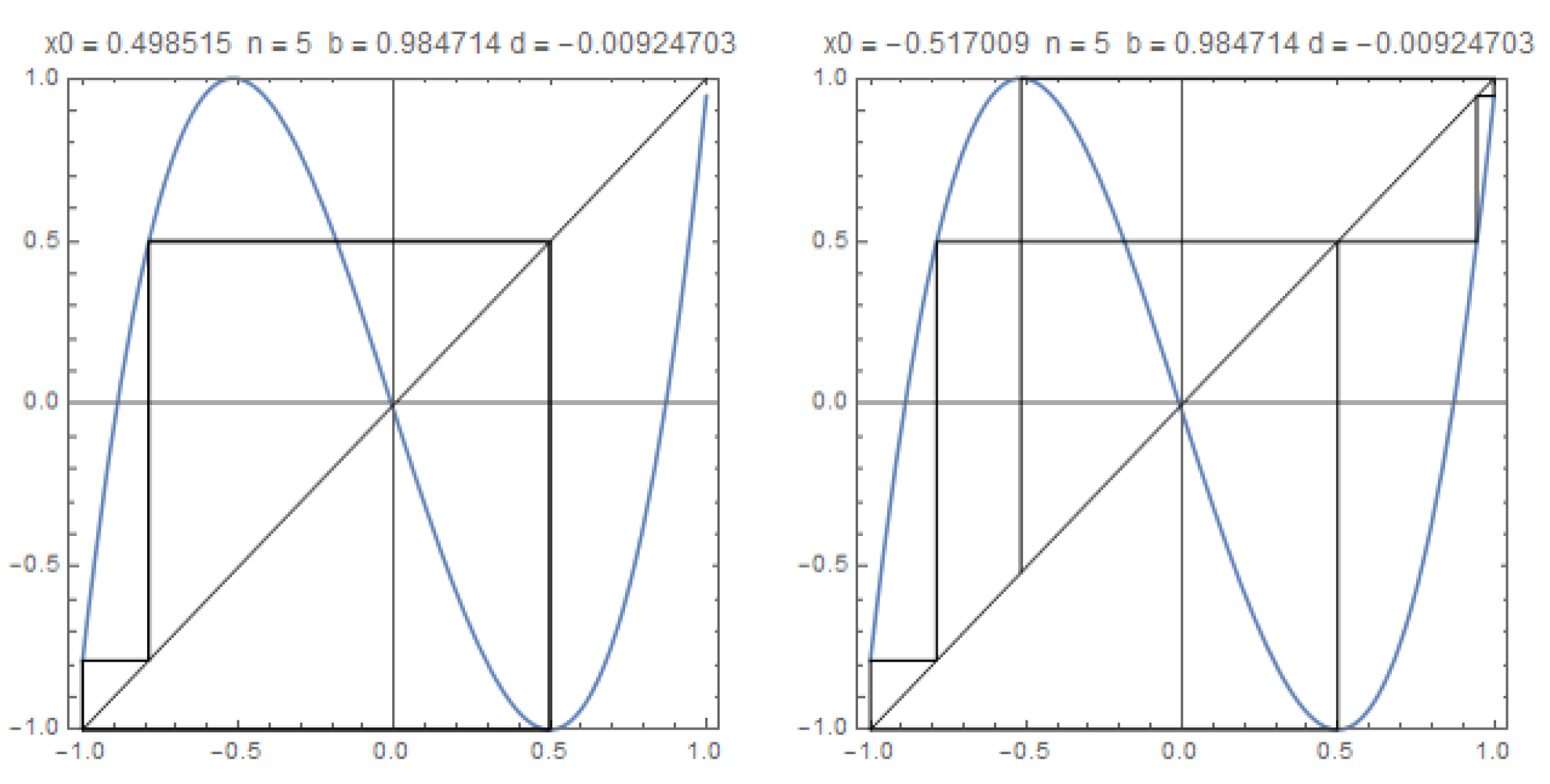
Example 1.
Let and so that , see Figure 5. In this case the shifted kneading sequences are,
and its ordering, as in (5) and (6), is
Note that . Also note that since we have .
The orbit of the critical point is, approximately
The orbit of the critical point is, approximately
Joined the two orbits and reordered
The Markov partition is constituted by the intervals, indexed by the Markov states
and the transition matrix is
Its Perron eigenvalue is precisely which corresponds to the growth number of the system. Therefore, the topological entropy is . The Markov states in terms of admissible words in the alphabet are
4. Isentropic Motion and Unique Attractor Cases
The topological entropy, as discussed previously, is a topological invariant for the dynamics of . In the symmetrical case, with , the map is characterized by the topological entropy, up to topological conjugacy. In the non-symmetric case, with the drift parameter , this is no longer true. We have for different values of possible dynamics, non equivalent in terms of topological conjugacy, with the same topological entropy. Here, we do not make a systematic study on this issue, however we describe the main points. On the other hand, we discuss the cases for which there is only one attractor, that is, both critical orbits coincide at to some finite time instant. For further reading on isentropics of cubic maps see Reference [17] and also References [11,15,18].
4.1. Piecewise Linear Semi-Conjugation and Isentropics
To find isentropic systems, that is, values of the parameters , for which the topological entropy of and are equal, it is useful the semi-conjugation of with a two parameter piecewise linear family. The existence of this semi-conjugation was proven in Reference [14], see also References [11,18]. We can, with more or less effort, chose an appropriate form, in order to include the two situations and in the same map. This is accomplished with the following parametrization, considering ,
It is useful to distinguish the branches of , given by
The map has constant slope, its absolute value is s and it is surjective in the interval , similarly to . The parameters , s and r are topological invariants for the family , through a semi-conjugation between and , see Reference [11]. Consider the restrictions and
For these values of the parameters there are two singular points (discontinuous derivative) inside , and correspond to the region , with respect to . The value s is the growth number of and r is the topological invariant distinguishing between isentropics. In fact, for fixed s and variable r the dynamics are not topological equivalent, however, the topological entropy is the same and equal to . These type of invariants were studied in various contexts by Sousa Ramos and his collaborators, see the review in Reference [16].
Note that the symbolic dynamics for these maps is equivalent to the formalism introduced to . We here use the same notation for the address map , the itinerary and the kneading invariant . The address of is then defined by
Again, if there is no danger of confusion we drop the index in the address map, that is, . The itinerary of a point x, which collects the addresses of the points in the orbit of x, is defined by
where and . The main difference to the differentiable bimodal family is that there is no attractive interval , and there are no windows of stability around the periodic critical orbits.
The isentropic kneading invariants are obtained fixing s and varying either or r. We can determine the parameters , so that , obtaining the parameters as function of the –invariant, with the topological entropy, , fixed:
See Figure 2, for examples with , for various values of r, . Therefore, the topological entropy is equal to , in every case. See the Example 2 in the next section to obtain the parameters for this case.
4.2. Unique Critical Orbit
The cases in which there is a unique attractor, that is, a unique critical orbit, are important since we may describe the behavior of the system specifying less information than with two arbitrary attractors. There are two possible situations in which the two critical orbits coincide: either both are periodic and coincide exactly or they coincide only at some time instant k, after some transient phase. In the first case the kneading sequences are of the type
and in the second case the kneading sequences are of the type
where P and Q are some admissible words of size . This corresponds to a situation in which
if , , or
if and .
Recall that the itineraries of the points correspond to the itineraries of the images of the critical points , since and are surjective on .
We will focus on the case , and therefore . The periodic case, including the case when S is a periodic sequence in (9), can be handled also by the topological Markov chain method explained in the previous section. However, the method described below is more direct to find s and r. Let us consider that the size of P is equal to and that S is periodic. Therefore, the parameters and must be so that
Recall that when then , and , and when then , and . Let us start with the symmetrical case: we immediately observe that, since the kneading sequences must be symmetrical, we have
Now, given let . Note the reverse order in which the symbols appear.
The following result allow us to identify isentropic kneading sequences and the corresponding topological invariants, see Reference [18] for more details.
Lemma 1.
Let and . Then is a polynomial on s which does not depend on r.
Proof.
Let , for , and recall that the sign function of each symbol in can be written depending on : , , . Then given an admissible word we have
Since for every , and the differences , , do not depend on r, we have that
does not depend on r. □
Note that if we set we may enunciate the result: the quantity is independent on r, for any admissible , therefore the result is valid for . From the Lemma 1, the parameter s can be determined by the equation
The parameter r can be determined by
or by
from the periodicity of S.
Example 2.
If
for both , we have from the condition (10)
which is a condition independent on r and on ρ. Therefore, for different r, ρ we have fixed topological entropy . The kneading sequences correspond to sequences in the form
for some S so that is a maximal sequence and minimal, in the case . The case , has always fixed kneading invariant and correspond to two re-scaled copies of the full tent map. Therefore, through the semi-conjugacy, we obtain the same kneading sequences for and the associated condition is
This give the parameter relation
which are the equations determining the isentropic curves in Figure 3, connecting the points marked and . For maps with parameters satisfying the previous relation the topological entropy is equal to .
Example 3.
Let us now consider the case . There are two cases: for , with
and for , with
The conditions on are obtained, with , through
and for , through
The solution greater than 1 is
for both . Let us consider two concrete examples with . The case is given by , obtaining
Let . Note that or , since the map is continuous. From (11) we have a condition to determine r which is
Therefore, in this case
Through the semi-conjugacy, we obtain the same kneading sequences for , and the associated condition on the parameters is given by
with the additional condition of the curve being contained in the region for and in the region for . The corresponding kneading invariants are of the type
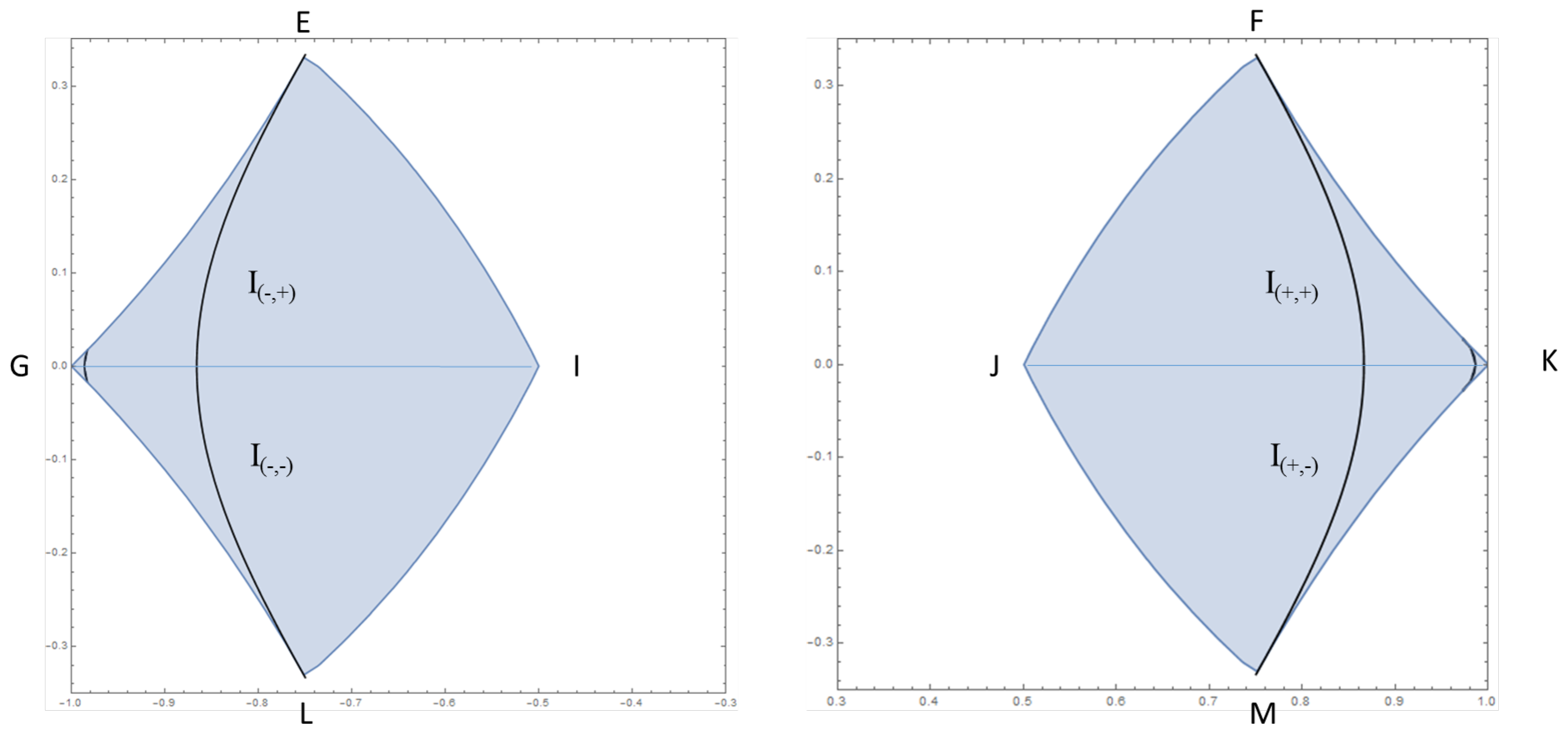
with , and
with . Using the equation above we represent the isentropic curves for in Figure 3. The curves are near the points G and K.
5. The Model—Cartesian Plane Motion
5.1. Definition
The trajectory of the animal is composed of patches of linear motions intertwined by changes of direction. The lengths and the directions of each patch are determined, in the Cartesian coordinates, by the iteration of the map
depending on the parameters and considering an external parameter, which does not affect the dynamical behavior. In an explicit way,
The position of the animal is, at each step , given by the coordinate vector . On the other hand, the displacement vector , at step k, codifies the future action of the animal. The parameter b characterizes the complexity of the motion, the parameter d characterizes its average drift and the parameter gives the scale of the motion and can be related with the energy spent during the motion. Note that the absolute value of the maximal displacement is normalized to 1. Therefore, re-scales whenever needed to the appropriate size. Recall that we assume there is a maximal step possible, for a given animal. In resume, the initial position of the animal is and the initial conditions for the state of the system, which determines the trajectory, is the pair .
Associated to is the kneading invariant, , through , which characterizes the global behavior of the animal, that is, the information which characterizes 1D dynamics is also characterizing 2D trajectories.
5.2. Interpretation of the Model
An animal in different circumstances, or time instants, produce different trajectories. We expect that under the same exterior conditions, more or less controlled, and with the same internal conditions (health, metabolism, etc.) the animal produce, not equal, however similar trajectories. In our model this corresponds to consider different initial state conditions . In the chaotic regime, due to sensitivity of the initial conditions, very close initial displacements can lead to very different trajectories, however with common topological invariants, see the Figure 6 for an example. The type of trajectory is determined by the values of the parameters , and what is equivalent the kneading invariant .
In isolated situation, , if the same animal is in a different internal state, with hunger, exhausted, aggressive, or other, we may expect that produce very different types of trajectories. These different behavior states are associated with different values of b. Therefore, a specie can be characterized by a set of possible parameters according to its observed behavior states. Moreover, a different specie can have a set of possible parameters , according to some of the strategies typical of the considered specie. Since there are different values of the parameter b producing topological equivalent behavior, corresponding to the windows of stability, in fact is preferable to make the correspondence between kneading sequences and behaviors. It is this correspondence that may be meaningful. We, thus, expect to have a specie characterized by a finite set of kneading invariants
ordered by topological entropy which coincides with the symbolic order, which may be associated with the typical behaviors according to internal and/or special controlled external conditions in quasi isolation. For example, may represent the simplest possible type of behavior, the rest. Next, , may codify directed trajectories, for example traveling. The next sequence, , may codify search for food or for a reference, and so on. The last, , may codify a random type behavior.
When the animal is not isolated, excluding for now interactions between animals or time dependent interactions, we may consider a constant interaction such as a air current, water current, temperature gradient, or other. This means that the parameter d is different from 0 and produces a tendency for displacements in one direction of the Cartesian coordinates. In this case, using the topological invariants , which can be computed directly from the kneading sequences as we have seen in Section 4, we have the possibility of establishing a set of kneading sequences, organized in increasing topological entropy, or, on the other hand, a set of kneading sequences with fixed topological entropy ordered by the –invariant which is related with the drift.
Moreover, as we have discussed in the section on isentropics, there are certain special values of the parameters for which the critical orbits coincide and this allows a particularly simple process to characterize the trajectories, since we are in fact using only one kneading sequence with the tail S and a word P, which characterize the transient behavior. This aspect may be very important to optimize procedures to obtain an approximate characterization of empirical data. It is much more simple to fit to a unique symbolic sequence, than having the possibility of varying the two sequences.
5.3. Pure and Mixed Bimodal Trajectories
Although isotropy is considered in assumption (6) it does not mean there are no geometrical patterns with preferential directions. In fact, these patterns may occur for certain values of the parameters and are artificial, consequence of the very simplified version of the model with uncorrelated Cartesian coordinates used. For certain types of parameters there are some tendency movements along the Cartesian axis and the diagonals, see for example the intermittent case in the dictionary, Figure 23 and the movements close to periodic orbits, for example Figure 18. Note that the fact the straight lines, which are also obtained for certain values of the parameters, are usually aligned with the Cartesian axis or the diagonals. Since we does not have apriori settled a reference frame, and if we observe an animal moving in a certain line or a maximal length occurs in a certain direction, we simply consider that this line is a Cartesian axis or a diagonal for the reference frame of the animal, in that section of the trajectory. On the other hand, since the model is built using uncoupled Cartesian coordinates, we must consider that the orientation of the reference frame for Cartesian coordinates may be changing.
For a fixed set of parameters and an orientation of the Cartesian frame, the obtained trajectories are called pure bimodal trajectories. It may happen that, even in the isolated situation, the animal by an internal strategy can alternate types of trajectories. Therefore, eventually the parameters or the orientation can be changing with some dynamical rule. The trajectories obtained by this process are called mixed bimodal trajectories. This issue will be explored in detail in a next work, in particular, towards the development of experimental procedures. See in the Figure 7 an example of two pure bimodal trajectories, with the same parameters and with a change in the orientation of the Cartesian frame, , obtaining a mixed bimodal trajectory. Figure 8 shows a mixed bimodal trajectory with changing parameters, in which the change can be due to internal state change (since ) or due to some external singular perturbation.
5.4. Scale, Uncertainty and Precision in the Trajectory Determinacy
When considering finite size animals the very small steps which may be produced by the iteration of the cubic, for certain values of the parameters as in the case of intermittent behavior, are not observed or observable—see in the dictionary in Figure 16 or 23. We may consider that there is a scale break at some point, that is, there is a limit scale for say below which there is no distinction in the details of the motion. In this case, the uncertainties regarding position, below this value, may be discarded. On the other hand, in real behavior, even in an almost isolated situation, gives origin to trajectories which do not fit those produced theoretically. The bimodal trajectories can be seen as templates or ideal geometrical objects which guide the real trajectories. Therefore, although the exact positions of the animal are not given by the coordinates determined by the numerical model, the global behavior is characterized by it. This may lead us to a similar procedure as in the stochastic methods. However, here we do not apriori give a distribution for the lengths and direction, instead the (pseudo)stochastic behavior is produced by the nonlinear iterated map.
Thus, for empirical use, instead of a pure one dimensional trajectory patch we may consider a region where the animal may be present, during the displacement, and the movement is guided by the bimodal trajectory, in the sense that the sequence of regions of possible occupancy is being determined by the iterated map. We may assume further that there is a region of possible turning point locations. The more natural way to accomplish this objective is to substitute a linear step by a region which includes the bimodal displacement vector in which there is a positive probability that the animal will be present.
A natural choice, however not unique, is to consider the rectangle which contains the displacement vector in the center and in the starting and ending positions to consider a disk of a certain diameter, which can be equal or not to the size of the rectangle. We may discuss the appropriate probability distribution. However, for now we simply consider that the animal has the possibility of being in the determined region. Therefore, given a position vector and a displacement vector , let be the unit vector orthogonal to . Consider the following points
The enveloping rectangle is determined by the vertices and ,
and the position disk
Therefore, for applications, instead of considering an exact trajectory it should be considered a sequence of rectangles, with the characteristic lengths and displacement vector length, a sequence of position disks, with characteristic length , which give a region of confidence containing real trajectories arising from sampling. Naturally, the smaller the accuracy parameters, , , the closer the sampled trajectories are to the theoretical bimodal trajectories. See the Figure 9, where an hypothetical empirical trajectory and its bimodal trajectory region are detailed.
This procedure, in addition, gives a method to estimate the area covered by the animal, estimating the number of rectangles and disks from above and from below subtracting a disk or a square of area every time there is an intersection.
Example 4.
Let us consider the following parameters , , which give , …. The length of the enveloping rectangle is and the radius of the position disk is . The trajectory is represented in Figure 10 is obtained with , , , . Note the enveloping region around the bimodal trajectory. The theoretical trajectory is represented in black lines and an hypothetical real trajectory which is contained in the rectangles and disks, whatever may be geometrically, is characterized by the same topological invariants.
6. Dictionary
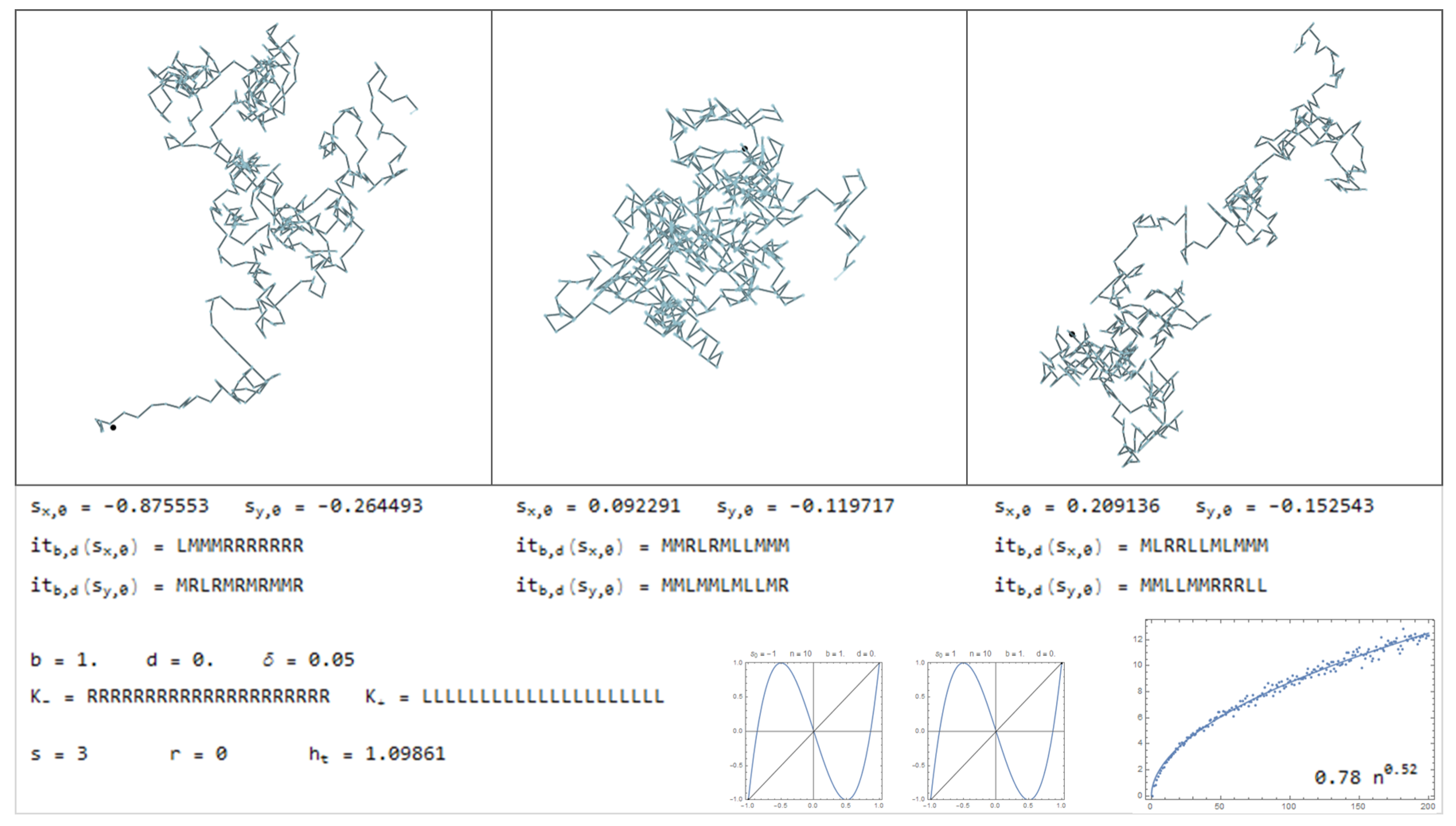
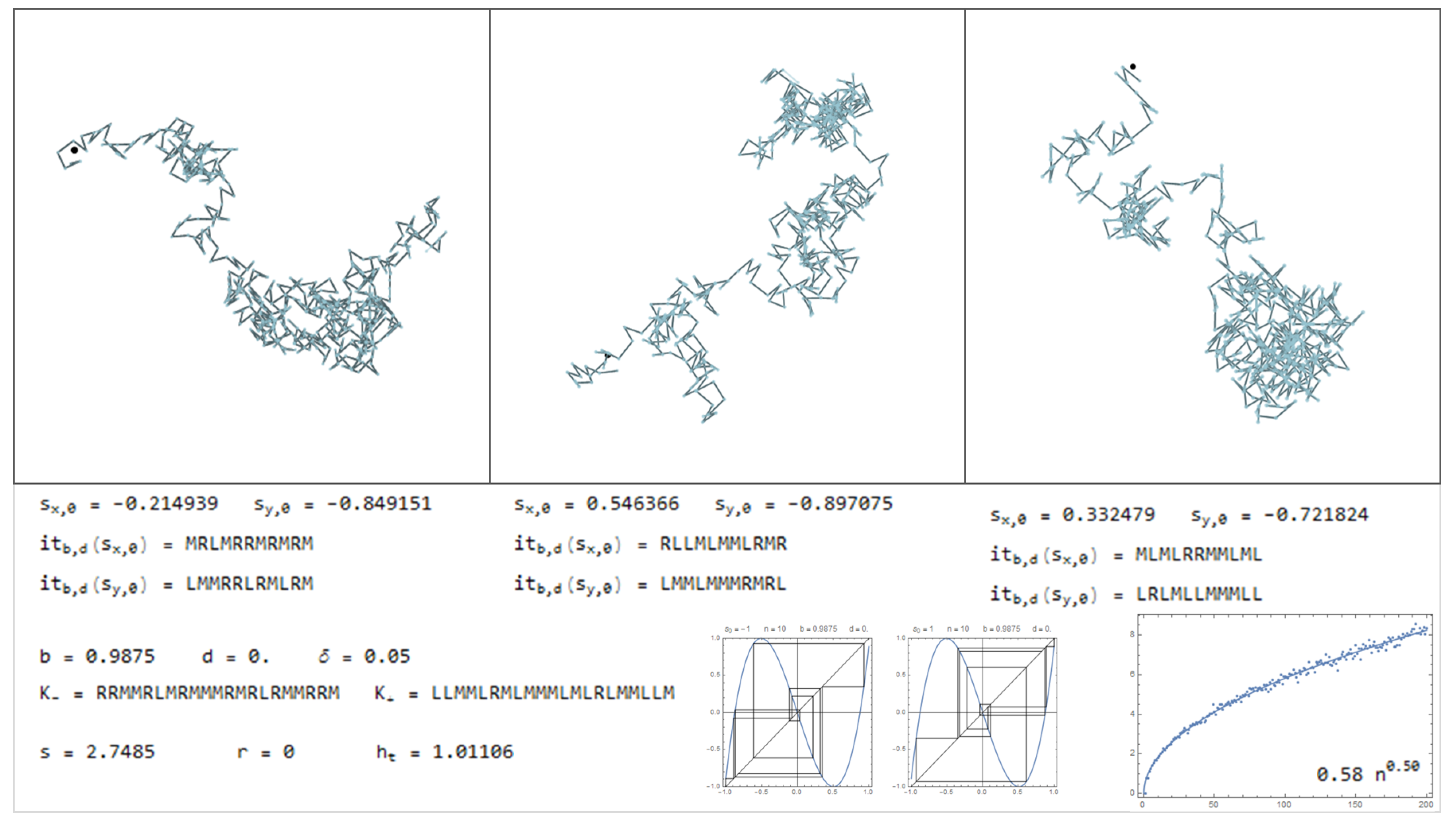
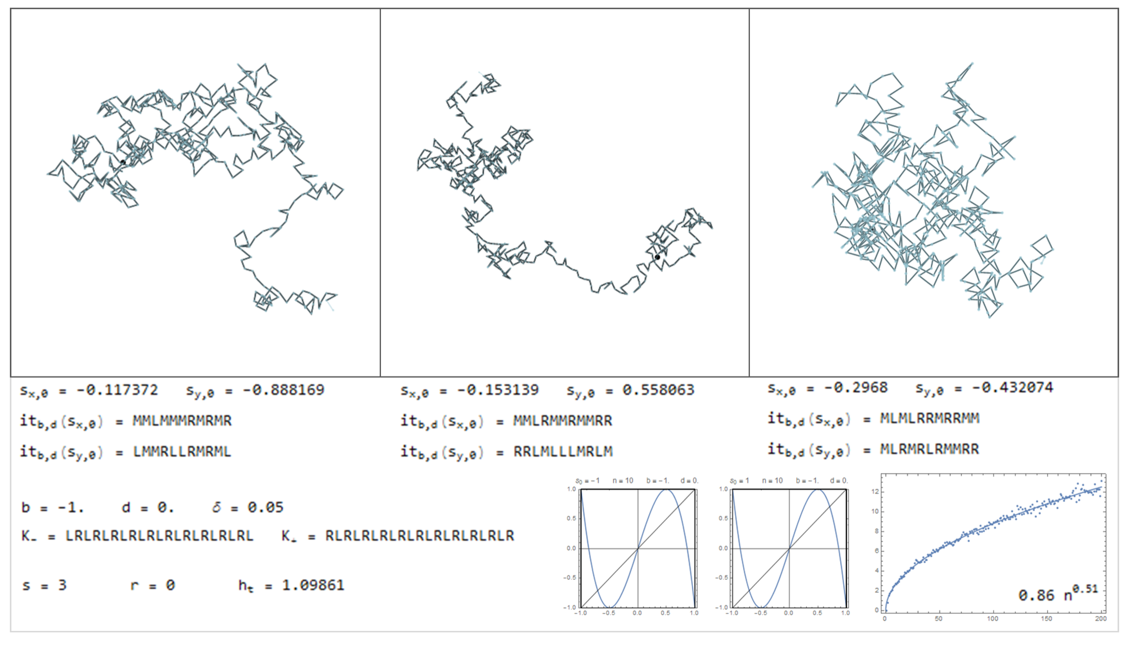
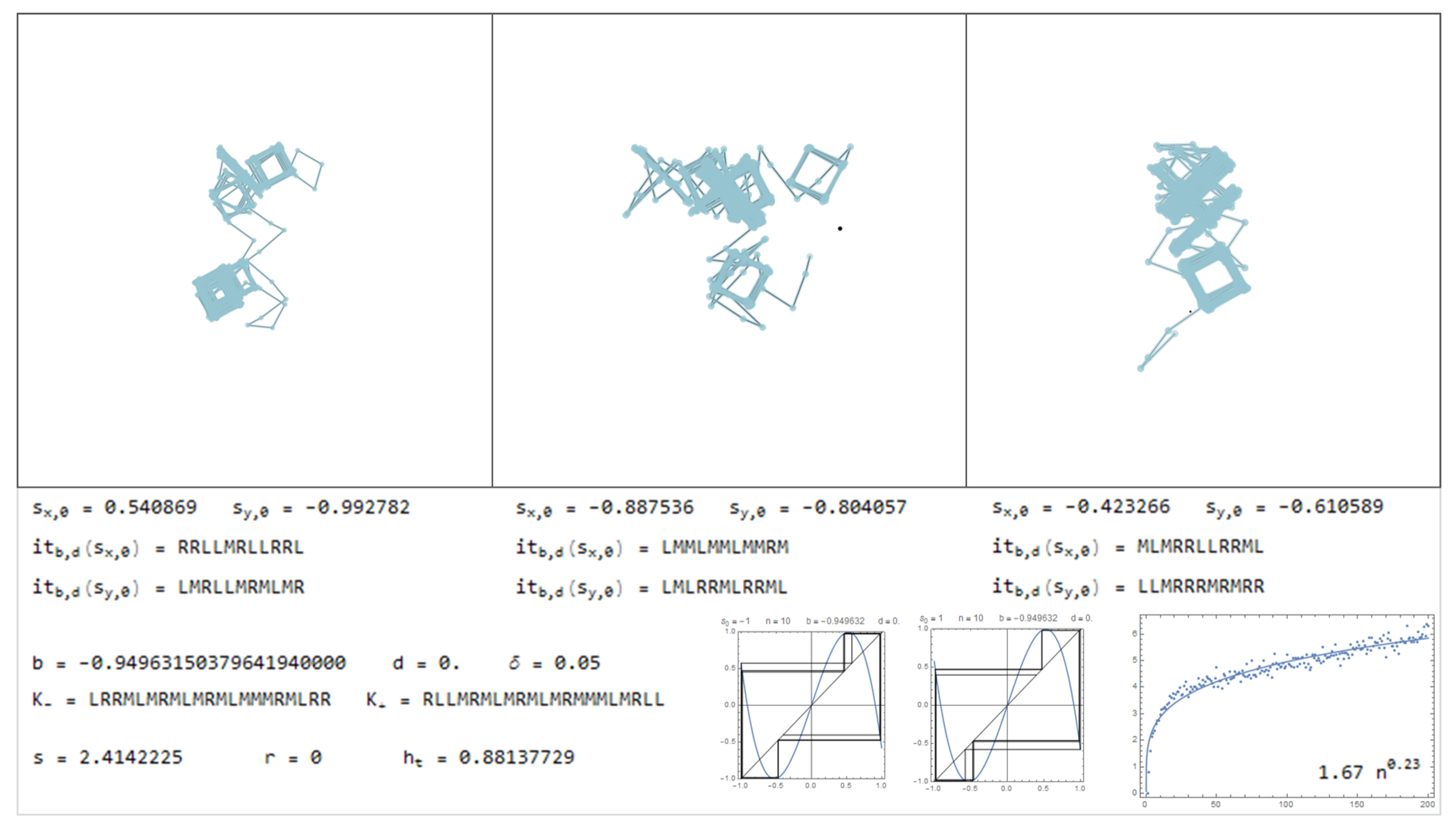
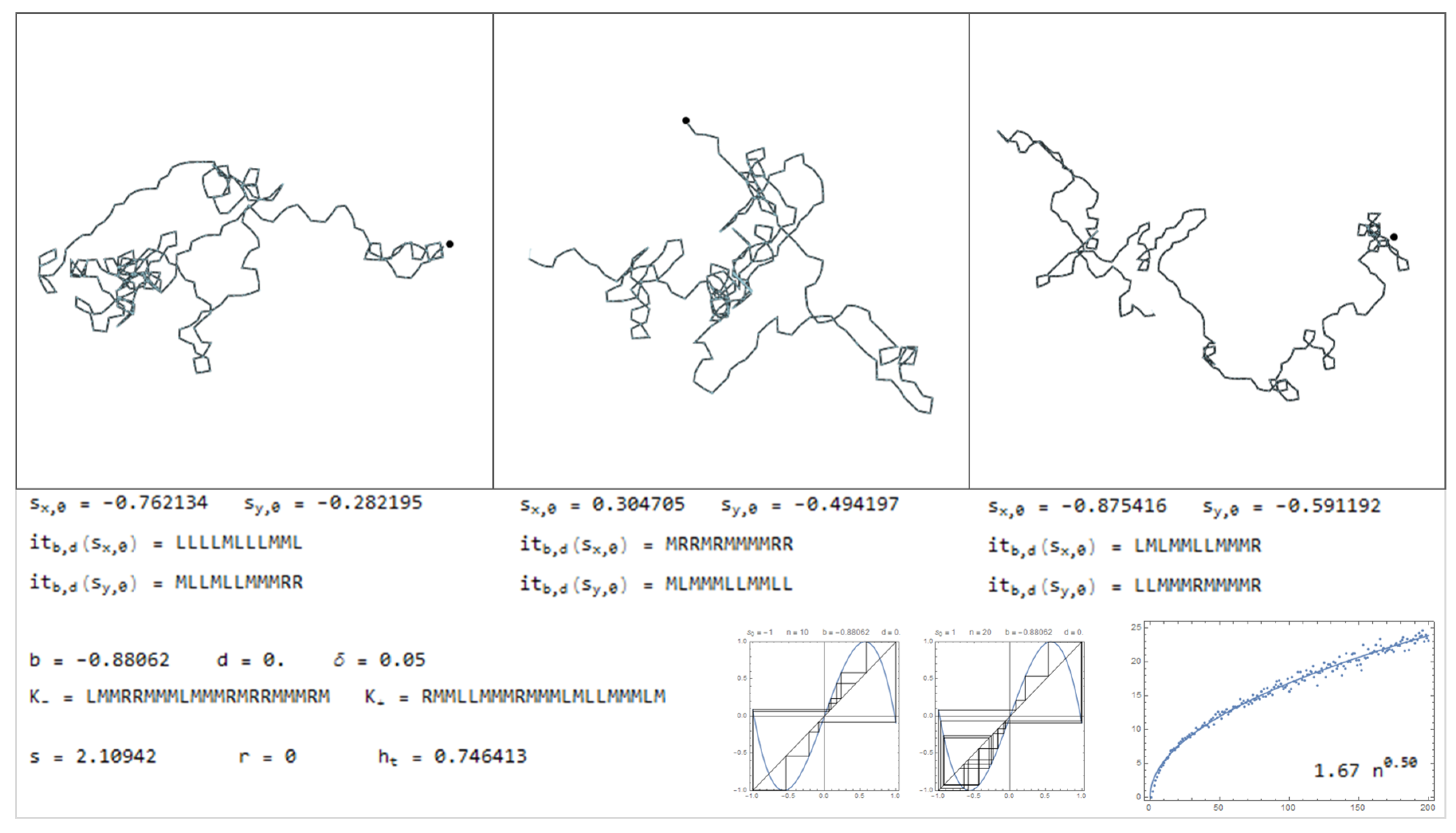
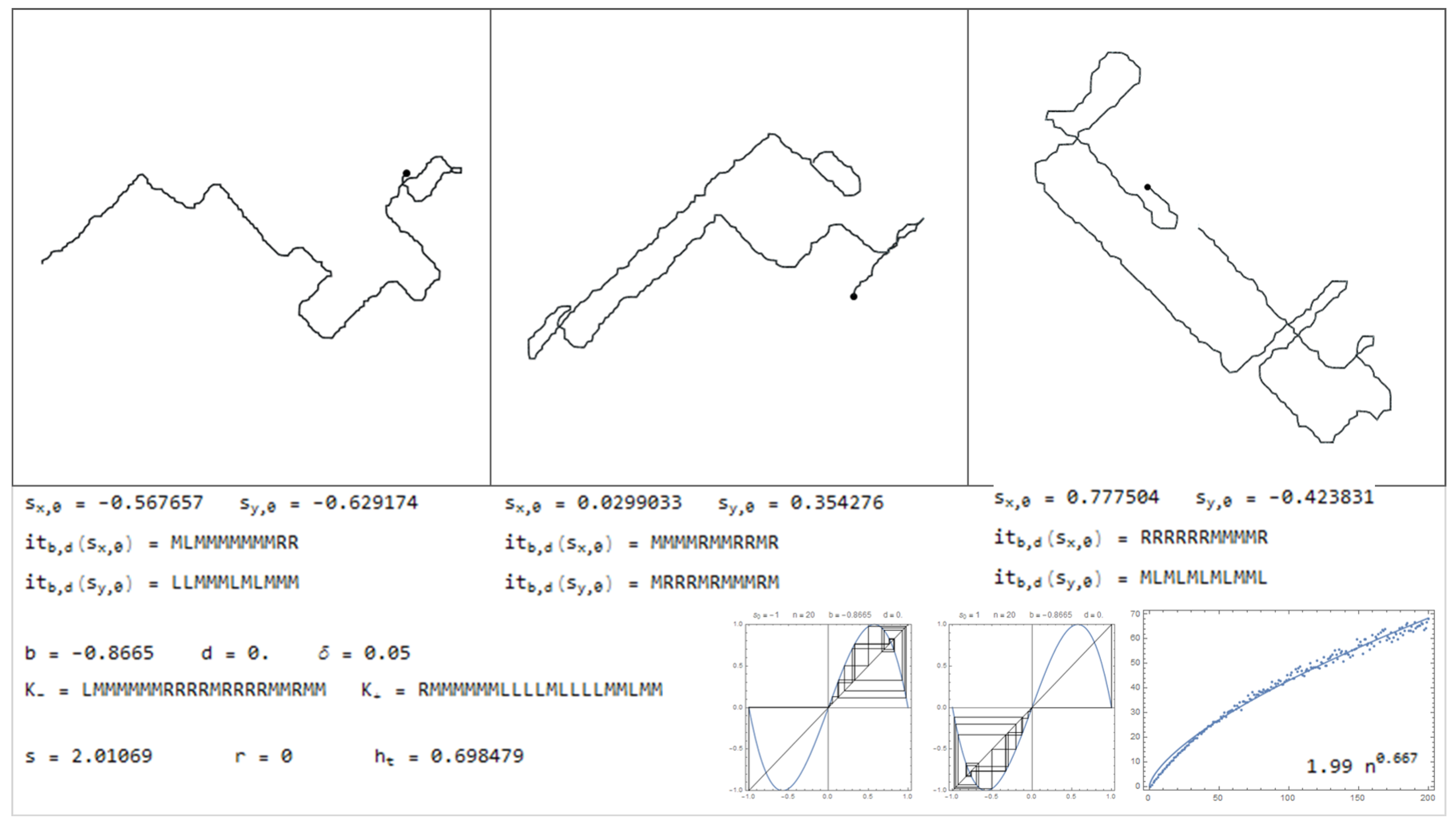
In this section is presented a sample of the dictionary, through Figure 11, Figure 12, Figure 13, Figure 14, Figure 15, Figure 16, Figure 17, Figure 18, Figure 19, Figure 20, Figure 21, Figure 22, Figure 23, Figure 24, Figure 25, Figure 26 and Figure 27, where examples of pure bimodal trajectories are illustrated, given the parameters . Some representative behaviors were chosen, there are many more. The key to read the dictionary is the following:
The values of the parameters are presented together with the corresponding kneading sequences. For each pair, , are shown three different simulations, with the initial conditions , chosen randomly. Note that due to the sensitivity to the initial conditions, in particular for high topological entropy, the trajectories change significantly with a very slight change in the initial conditions. In Figure 11, Figure 12, Figure 13, Figure 14, Figure 15 and Figure 16, are represented trajectories with positive b and . In Figure 17, Figure 18, Figure 19, Figure 20, Figure 21, Figure 22 and Figure 23, are represented trajectories with negative b and . In Figure 24 and Figure 25 both the parameters are positive and in Figure 26 and Figure 27 the parameter b is negative and d is positive. The topological invariants are also presented, such as growth number s, the r-invariant and the topological entropy. Two graphics of the trajectories of the critical points, under the map are presented, to illustrate the global behavior of the produced displacements. Finally, a simulation which determine approximately the quadratic mean displacement. This shows that for different values of the parameters the behavior, in average, may be comparable to the random walk, that is, diffusive behavior with the exponent close to . This is the case in Figure 11, Figure 12 and Figure 13 and Figure 15, for example. There occurs superdiffusive behavior with exponent larger than and below 1, for example in Figure 16, Figure 23 and Figure 24. The sub-diffusive behavior appears with the exponent less than . This is usually associated to parameters producing atractive orbits close to periodic orbits which have no zero average, producing a slow drift, although d may be 0. For an example of this phenomena see Figure 19 and Figure 21. Naturally, there are values of the parameters where the displacement is quasilinear. In this case, it is an almost direct trajectory with low (or 0) topological entropy.
Considering the symmetric bimodal does not mean that a particular trajectory does not exhibit a tendency to a certain direction. Means that if many different trajectories are produced, with random initial conditions, in average there is no preferential direction. Instead, with the drift () there is this tendency that almost all trajectories gives a preferential direction, related with d.
7. Conclusions, Discussion and Future Work
The objective of the present paper is to further develop the model introduced in Reference [10], used to simulate and classify different types of trajectories of organisms arising in biology. The model uses an iterated map of the interval—a cubic map - depending on two parameters . The map produces the displacements in each Cartesian coordinate through iteration. The produced trajectories are identified as typical or template paths of certain organisms which at some extent are isolated, with stable behavior, or exposed to a constant external influence. The characteristics, patterns or irregularities of the trajectories, arising from any physical conditions or organism behavior, are codified in the symbolic description of the orbits of , through the alphabet . The main classifying tool is the kneading invariant, , of the map . To a particular patch, or piece of trajectory, a symbolic sequence is associated. Thus, the study of the possible trajectories and its properties can be made enumerating symbolic sequences satisfying certain combinatorial constrains, given by the admissibility conditions in the section. On the other hand, using ergodic theory for symbolic dynamics and for iterated maps of the interval, the probability distributions can be derived as a consequence of the model.
Regarding the possible use of the model to analyze empirical data it is necessary to take the following into account. Particular observed animal trajectories are not necessarily reproduced in an exact manner by the model. From the pattern of an observed trajectory, are identified: (1) The consecutive steps where the direction is approximately maintained. (2) The changes in direction. (3) The consecutive steps of changing direction. Then, from this information, it is possible to produce a sequence in the referred alphabet , associated with the observed trajectory. It is then possible to determine a class of kneading sequences which turns the observed sequence into admissible, with respect to the bimodal criteria. In this case, the approximate values for the topological entropy and other invariants can be computed, obtaining a characterization of the system which produces similar trajectories, as the given one. This process still needs some details to be completed. A paper dedicated exclusively on dealing with experimental procedure to find the best way to fit the bimodal trajectories on empirical trajectories, is being prepared.
The constraints that are either external, such as terrain or medium type, or internal, such as metabolism, are codified and included in the kneading sequences and naturally on the parameter choice. The allowed and not allowed types of motions are determined by the combinatorial admissibility rules described in Section 3. The correspondence between the phenomena or experimental observations and the kneading sequences are not determined apriori, or deduced, they must be obtained through experimental procedure.
The generated motion in the case , is only dependent on the internal strategy, the metabolism of the animal, or on the stabilized physical conditions. Naturally, the same organism can behave differently if the physical conditions are different, and the parameter b characterize motions in those stable equilibrium environment. Therefore, b resumes organism behavior and the stable physical conditions of the environment. The parameter d is introduced to model the existence of a constant external gradient of any kind, provoking a constant drift in the trajectories. In future work it is intended to use this model to introduce interactions and to analyze how this interactions affect globally the motion. We can introduce time dependent interaction or a space dependent interaction, such as a potential. In this case the parameters will be dependent on the organism position
The uncertainty at the theoretical level, with respect to the initial conditions, influences the difference in the produced trajectories for the same behavior, organism or physical conditions. That is, a small perturbation of the initial conditions , , corresponds to perturbing a given trajectory, as in Figure 6, obtaining different runs of the same organism, for example. This allows the simulation of the movement of particular organisms in particular physical conditions, choosing different initial conditions for the same set of parameters. The uncertainty with respect to small perturbation of the parameters , depending on the parameter region, can influence deeply the behavior or the physical conditions for a given organism. This is typical for chaotic systems and can be observed in some of the dictionary entries in Section 6. Regarding uncertainty of experimental data, the relevant concept is the critical sequences of lengths, in each Cartesian coordinate, associated with the maximal lengths observed. These sequences constitute the kneading invariant. The important point is to identify how the consecutive observed lengths organize themselves with respect to the critical lengths, that is, if are larger (symbol R), smaller (symbol L) or between the two critical lengths (symbol M). The symbolic dynamics is robust to uncertainty regarding individual length measurements. However, regarding the choice of the sample points, see for example Figure 9, and the choice of the turning points of the rotation in the Cartesian frame, from an empirical trajectory, some work must be done to decide if the obtained results are somehow independent on sampling method or if it is necessary to develop a canonical sampling procedure adapted to the model.
This method can be easily generalized to three dimensions, as was suggested in Reference [10].
It is planned also to explore the same method, iterated interval maps, in different coordinate systems, namely polar coordinates, or different iterated maps, not necessarily bimodal, or continuous.
Funding
This work was supported by FCT—Fundacao para a Ciencia e a Tecnologia under the project UID/MAT/04674/2019.
Acknowledgments
The author thanks the anonymous referees for their comments which improved this manuscript.
Conflicts of Interest
The author declares no conflict of interest.
References
- Smouse, P.E.; Focardi, S.; Moorcroft, P.R.; Kie, J.G.; Forester, J.D.; Morales, J.M. Stochastic modelling of animal movement. Philos. Trans. R. Soc. B 2010, 365, 2201–2211. [Google Scholar] [CrossRef] [PubMed] [Green Version]
- Nathan, R.; Getz, W.M.; Revilla, E.; Holyoak, M.; Kadmon, R.; Saltz, D.; Smouse, P.E. A movement ecology paradigm for unifying organismal movement research. Proc. Natl. Acad. Sci. USA 2008, 105, 19052–19059. [Google Scholar] [CrossRef] [PubMed] [Green Version]
- Tang, W.; Bennett, D.A. Agent-based modeling of animal movement: A review. Geogr. Compass 2010, 4, 682–700. [Google Scholar] [CrossRef]
- Jonsen, I.D.; Flemming, J.M.; Myers, R.A. Robust state–space modeling of animal movement data. Ecology 2005, 86, 2874–2880. [Google Scholar] [CrossRef]
- Patterson, T.A.; Thomas, L.; Wilcox, C.; Ovaskainen, O.; Matthiopoulos, J. State–space models of individual animal movement. Trends Ecol. Evol. 2008, 23, 87–94. [Google Scholar] [CrossRef] [PubMed]
- McClintock, B.T.; King, R.; Thomas, L.; Matthiopoulos, J.; McConnell, B.J.; Morales, J.M. A general discrete-time modeling framework for animal movement using multistate random walks. Ecol. Monogr. 2012, 82, 335–349. [Google Scholar] [CrossRef] [Green Version]
- Langrock, R.; King, R.; Matthiopoulos, J.; Thomas, L.; Fortin, D.; Morales, J.M. Flexible and practical modeling of animal telemetry data: Hidden Markov models and extensions. Ecology 2012, 93, 2336–2342. [Google Scholar] [CrossRef] [PubMed]
- Petrovskii, S.; Mashanova, A.; Jansen, V. Variation in individual walking behavior creates the impression of a Lévy flight. PNAS 2011, 108, 8704–8707. [Google Scholar] [CrossRef] [PubMed] [Green Version]
- Tilles, P.F.; Petrovskii, S.V.; Natti, P.L. A random walk description of individual animal movement accounting for periods of rest. R. Soc. Open Sci. 2016, 3, 160566. [Google Scholar] [CrossRef] [PubMed] [Green Version]
- Ramos, C. Animal movement: Symbolic dynamics and topological classification. MBE 2019, 16, 5464–5489. [Google Scholar] [CrossRef] [PubMed]
- Almeida, P.; Lampreia, J.P.; Ramos, J.S. Topological invariants for bimodal maps. In ECIT 1992; World Sci. Publishing: Batchuns, Austria, 1996; pp. 1–18. [Google Scholar]
- Lampreia, J.P.; Sousa Ramos, J. Symbolic dynamics of bimodal maps. Port. Math 1997, 54, 1–18. [Google Scholar]
- Lampreia, J.P.; Severino, R.; Sousa Ramos, J. Irreducible complexity of iterated symmetrical bimodal maps. Discret. Dyn. Nat. Soc. 2005, 1, 69–85. [Google Scholar] [CrossRef]
- Milnor, J.; Thurston, W. On Iterated Maps of the Interval. In Dynamical System; Alexander, J.C., Ed.; Procededings Univ. Maryland 1986–1987, Lect. Notes in Math. n.1342; Springer: Berlin, Germany, 1988. [Google Scholar]
- Lampreia, J.P.; Severino, R.; Ramos, J.S. Renormalizations for cubic maps. Ann. Math. Silesianae 1999, 13, 257–270. [Google Scholar]
- Sousa Ramos, J. Introduction to Nonlinear Dynamics of Electronic Systems: Tutorial, Nonlinear Dynamics; Springer: Berlin, Germany, 2006; Volume 44, pp. 3–14. [Google Scholar]
- Milnor, J.; Tresser, C. On entropy and monotonicity of real cubic maps. Comm. Math. Phys. 2000, 209, 123–178. [Google Scholar] [CrossRef] [Green Version]
- Martins, N.; Severino, R.; Sousa Ramos, J. Isentropic real cubic maps. Int. J. Bifurc. Chaos 2003, 13, 1701–1709. [Google Scholar] [CrossRef]
Figure 1.
Space of parameters with the dynamical behavior specified.

Figure 2.
Graphs of for , and , on the left and for , on the right. The growth number is equal to 2 in every case, and, therefore, give origin to the same topological entropy Note that , in every case.
Figure 2.
Graphs of for , and , on the left and for , on the right. The growth number is equal to 2 in every case, and, therefore, give origin to the same topological entropy Note that , in every case.

Figure 3.
The region with the isentropes represented as black curves: for , the two largest curves connecting the points and , and for the smallest curves near the points G and K.
Figure 3.
The region with the isentropes represented as black curves: for , the two largest curves connecting the points and , and for the smallest curves near the points G and K.

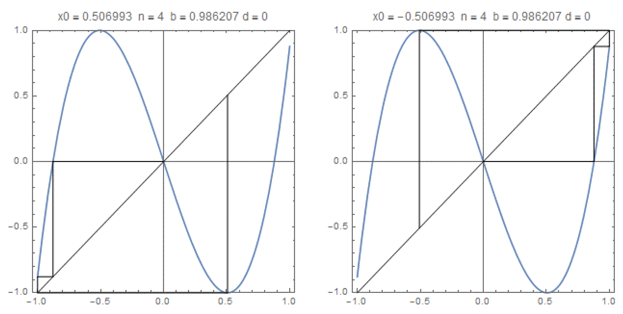
Figure 4.
The graphics of with the trajectories of the critical points, and in the case , the kneading invariant is The growth number is and
Figure 4.
The graphics of with the trajectories of the critical points, and in the case , the kneading invariant is The growth number is and

Figure 5.
The graphics of with the trajectories of the critical points, and in the case the kneading invariant is The growth number is and .
Figure 5.
The graphics of with the trajectories of the critical points, and in the case the kneading invariant is The growth number is and .

Figure 6.
For parameters and , the initial conditions and lead to different trajectories after few time steps. In this case approximately 20 time steps.
Figure 6.
For parameters and , the initial conditions and lead to different trajectories after few time steps. In this case approximately 20 time steps.

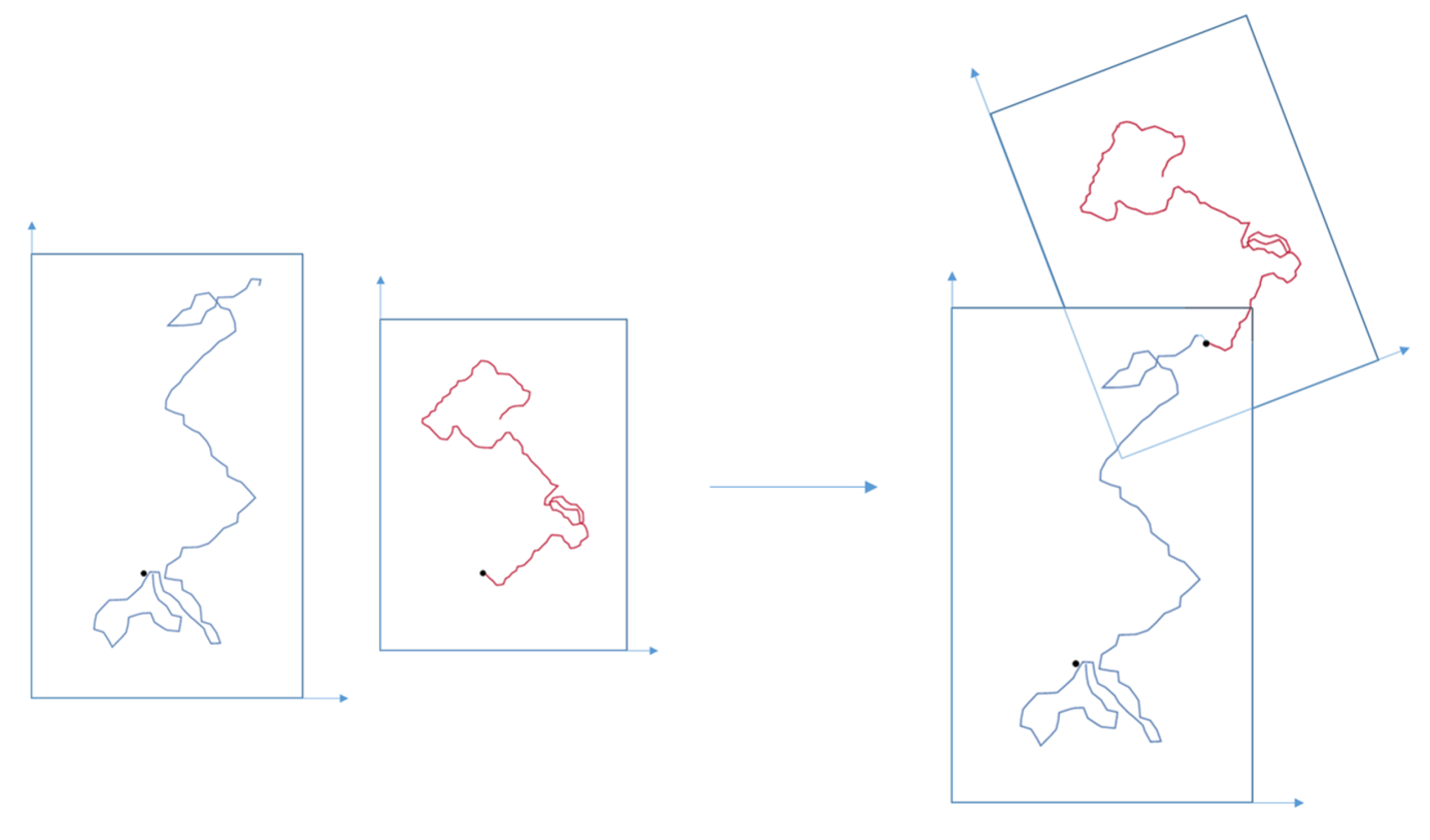
Figure 7.
Two patches of pure bimodal trajectories with the same parameters , which compose the mixed bimodal trajectory on the right, with a rotation of between them.
Figure 7.
Two patches of pure bimodal trajectories with the same parameters , which compose the mixed bimodal trajectory on the right, with a rotation of between them.

Figure 8.
Two patches of pure bimodal trajectories with the different parameters , on the left, , on the right, which compose the mixed bimodal trajectory on the right, with a rotation of between them.
Figure 8.
Two patches of pure bimodal trajectories with the different parameters , on the left, , on the right, which compose the mixed bimodal trajectory on the right, with a rotation of between them.

Figure 9.
Trajectory region obtained by the iteration of the map , with and , for the dimensions of the rectangular regions and disks respectively. On the left an example of an eventual real trajectory and in the middle the trajectory fitted into the pure bimodal trajectory region.
Figure 9.
Trajectory region obtained by the iteration of the map , with and , for the dimensions of the rectangular regions and disks respectively. On the left an example of an eventual real trajectory and in the middle the trajectory fitted into the pure bimodal trajectory region.

Figure 10.
Trajectory obtained with , , , , and , for the dimensions of the rectangular regions and disks respectively. The real trajectory is contained inside the region determined by the sequence of rectangles and disks. Therefore, the characteristic lengths and give an estimate of the precision involved in the measurements.

Figure 11.
Trajectories produced with and .

Figure 12.
Trajectories produced with and .

Figure 13.
Trajectories produced with and .

Figure 14.
Trajectories produced with and .

Figure 15.
Trajectories produced with and .

Figure 16.
Trajectories produced with and .

Figure 17.
Trajectories produced with and .

Figure 18.
Trajectories produced with and .

Figure 19.
Trajectories produced with and .

Figure 20.
Trajectories produced with and .

Figure 21.
Trajectories produced with and .

Figure 22.
Trajectories produced with and .

Figure 23.
Trajectories produced with and .

Figure 24.
Trajectories produced with and .

Figure 25.
Trajectories produced with and .

Figure 26.
Trajectories produced with and .

Figure 27.
Trajectories produced with and .

© 2020 by the author. Licensee MDPI, Basel, Switzerland. This article is an open access article distributed under the terms and conditions of the Creative Commons Attribution (CC BY) license (http://creativecommons.org/licenses/by/4.0/).
Share and Cite
MDPI and ACS Style
Correia Ramos, C. Kinematics in Biology: Symbolic Dynamics Approach. Mathematics 2020, 8, 339. https://doi.org/10.3390/math8030339
AMA Style
Correia Ramos C. Kinematics in Biology: Symbolic Dynamics Approach. Mathematics. 2020; 8(3):339. https://doi.org/10.3390/math8030339
Chicago/Turabian StyleCorreia Ramos, Carlos. 2020. "Kinematics in Biology: Symbolic Dynamics Approach" Mathematics 8, no. 3: 339. https://doi.org/10.3390/math8030339
Note that from the first issue of 2016, this journal uses article numbers instead of page numbers. See further details here.