Searching for Complexity in the Human Pupillary Light Reflex

Abstract

This article aims to examine the dynamical characteristics of the pupillary light reflex and to provide a contribution towards their explanation based on the nonlinear theory of dynamical systems. To introduce the necessary concepts, terminology, and relevant features of the pupillary light reflex and its associated delay, we start with an overview of the human eye anatomy and physiology with emphasis on the iris, pupil, and retina. We also present the most highly regarded models for pupil dynamics found in the current scientific literature. Then we consider the model developed by Longtin and Milton, which models the human pupillary light reflex, defined by a nonlinear differential equation with delay, and present our study carried out on the qualitative and quantitative dynamic behavior of that neurophysiological control system.

1. Introduction

As is widely known, since the concept of derivative was first developed, the ordinary differential equations have been used to model natural phenomena and they have provided a good approximation to determine its behavior. However, they involve functions and their derivatives that all evolve at the same time t. This is a feature that does not take into account the non-instantaneous nature of many phenomena. Additionally, phenomena with a delayed effect have been found. These phenomena are best modeled by a more general type of equations, the so-called delay differential equations (DDEs), making them one of the mathematical “tools” widely used in many applications ([1,2]). Such applications arise in a wide variety of fields as biophysics [3], biology [4], chemistry [5], climate [6] or even medicine [7], whenever it is essential to portray the non-instantaneous nature of the processes [8].

Within this framework, mathematical models for neural reflex mechanisms often take the form of a first-order DDE, that is

$$\dot{y}\left(t\right)=F\left(y\left(t-\tau \right)\right)-\alpha y\left(t\right),$$

where $y\left(t\right)$ and $y\left(t-\tau \right)$ are, respectively, the values of the controlled variables at time moments t and $t-\tau$, $\alpha >0$ represents a constant rate and F describes feedback action. Feedback action is one of the most important mechanisms for balancing, adjusting neural activity. Time delay $\tau$ is an essential feature of such relevant apparatus due to finite axonal conduction and neural processing times. Note that, while in a first-order ordinary differential equation, the derivative of the solution function relies on the solution function at current time moment t, in a first-order DDE the derivative is also determined upon the solutions obtained previously.

As it was showed by Longtin and Milton [9], the human pupillary light reflex (PLR) can be modeled through a nonlinear DDE where the solution function represents the pupil area. Note that several models of the human PLR have been constructed. These models take into account, either explicitly with the incident light as the variable ([10,11,12]) or implicitly [13], a number of important physical parameters obtained by experimental measurements: pupillary latency, constriction and velocity, and maximum and minimum pupil size, among others. However, the aim of this research was to take advantage of the dynamics of a DDE.

In a simplified way, human PLR is the pupillary response to variations in light intensity reaching the retina. As is briefly explained in Section 2, PLR is the neural feedback mechanism engaged for the reduction of the pupil area in high light environments and its increase in low light environments through the iris muscle activity. Feedback is negative because an increase in light causes a decrease in pupil size and vice versa. PLR is the constriction (dilation) of the pupil that is caused by an increase (a decrease) in the illumination of the retina (PLR and accommodation are the most noticeable involuntary movements of the human pupil, which reflect the change of its size. Accommodation is the pupillary response for focal length. There are also some spontaneous irregular fluctuations in pupil area called hippus, which occurs within a frequency range of $0.05$ to $0.3$ Hz.). The qualitative analysis of the relevant characteristics of the PLR, as well as its clarification, has been based on theoretical notions and computational (numerical) analysis of nonlinear dynamical systems. By considering some developments about the DDEs (Section 3) and the model presented by Longtin and Milton [9] (Section 4), the occurrence of oscillations in the PLR and their properties can be studied and the oscillatory phenomena highlighted by varying the level of complexity exhibited by the model (Section 5 and Section 6).

2. Pathways to PLR Feedback Control

The pupil is located in the iris center and works as a mobile opening that controls the amount of light that enters the eye and reaches the retina. Changes in pupil diameter adjust the level of retinal illumination and the depth of focus of the eye [14]. Pupil constriction (or miosis) occurs in response to increases in retinal illumination and during near viewing (see pupillary near response explained below). Pupil constriction also occurs with fatigue, drowsiness, or decreased alertness. Pupil dilation (or mydriasis) occurs both in response to decreases in ambient lighting and in stimuli or excitation of alertness. Depending on the relative balance of these conditions, pupil diameter can vary between $1.5$ and 8 mm in normal individuals, which corresponds to approximately a 28-fold change in the area.

The pupil diameter, more precisely the iris size, results from the action of two iris muscles, the circular sphincter pupillae, under the control of the parasympathetic nervous system, and the radial dilator pupillae, controlled primarily by the sympathetic nervous system ([15,16]). Namely, contraction of the sphincter pupillae, jointly with relaxation of the dilator pupillae, causes pupil constriction; whereas pupil dilation corresponds to contraction of the dilator pupillae and simultaneous relaxation of the sphincter pupillae [17]. These muscles of the iris are innervated by postganglionic neurons originating from the ciliary and upper cervical ganglia, which in turn receive preganglionic information from the Edinger-Westfall postganglia (EWpg) and intermediolateral. The central nervous system is the ultimate controller of both EWpg and inter-mediolateral, influenced by different variables such as retinal irradiance, viewing distance, alertness, and cognitive load. The light is captured through five (photo)receptors presented in the human retina that have distinct temporal signaling properties [18]: cones sensitive to long wavelengths (L), cones sensitive to medium wavelengths (M), cones sensitive to short wavelengths (S), rods and the so-called intrinsically photosensitive retinal ganglion cells (ipRGCs), more recently considered.

Based on the clinical manifestations of the defects in the PLR, the pathway control of pupil diameter has traditionally been separated into afferent and efferent. The afferent pathway is composed of both the contributions of rods and cones through the axons of the retinal ganglion cells that project into the pretectum and of ipRGCs cells that project bilaterally to the Edinger-Westphal nucleus. The efferent pathway is composed of the preganglionic pupilloconstriction fibers of the EWpg and their postganglionic recipient neurons in the ciliary ganglion, which innervate the iris sphincter pupillae.

It is appropriate to mention the pupillary near response, the particular case where the pupil constriction occurs after a change in viewing distance from far to close [14]. During near viewing, the eyes converge intending to bring the image of the object upon similar regions of each retina (convergent response), the refractive power of the crystalline lens is adjusted to focus on the retina (accommodative response), and the iris constricts reducing the diameter of the pupil (pupil constriction response). This collective process composed of three oculomotor responses has been classically termed the near triad (or near response).

The pupil is influenced by the cortical afferents that measure the nearby pupillary response as well as by the visual cortical regions and the non-visual cortical regions [18]. Small changes in the diameter of pupil take place during the presentation of visual stimuli such as colored stimuli, isoluminant, and gratings, as well as non-visual stimuli such as auditory tones, and even during superior cortical functions such as problem-solving. These facts provide clear evidence of cortical influence on pupil behavior, complying with complex aspects of visual stimuli such as movement, color, and texture.

3. Nonlinear Time-Delay Equations

Consider a first-order DDE with a single constant positive delay time $\tau$

$$\dot{y}\left(t\right)=G\left(y\left(t\right),y(t-\tau )\right),$$

(1)

where $y\left(t\right)\in \mathbb{R}$ and $t\ge 0$. As explained below, it is essential to consider some notes that allow us to understand a one-dimensional DDE as an infinite dimensional dynamic system ([19,20,21,22]) Without loss of generality we can assume delay time $\tau$ equal to 1

$$\dot{y}\left(t\right)=G(y\left(t\right),y(t-1)),$$

(2)

by means an appropriate rescaling of time t in equation (1).

For all $t\ge 0$ DDE (2) defines a unique solution function $y\left(t\right)$, just based on the initial data that must be given as $y\left(t\right)$ values for all $-1\le t\le 0$. Otherwise, its right-hand side will not be to be defined for some $t\in [0,1]$.

For Equation (2) to describe a well defined evolutionary process, we may consider that G is such that for any continuous initial function $\varphi :[-1,0]\to \mathbb{R}$, there exists a unique solution function $y\left(t\right)$ satisfying Equation (2) $\forall t>0$, and the initial condition

$$y\left(t\right)=\varphi \left(t\right),t\in [-1,0].$$

(3)

DDE (2) can be considered as a dynamical system defined in the infinite-dimensional phase space of continuous functions on the interval $[-1,0]$, $C[-1,0]$. More generally, the evolution of a solution function for $t>T$ is determined solely by its behavior in the interval $[T-1,T]$.

Consider the function

$$y_t\left(s\right)=y(t+s),\mathrm{for}s\in [-1,0]$$

(4)

that represents the part of a given solution function $y\left(t\right)$ on the delay interval $[t-1,t]$. As $y_t$ determines in a unique way $\dot{y}\left(t\right)$ when t belongs to $0\le t\le t^{\prime }$, it can considered that $y_t$ is the phase point (at time t) for the corresponding dynamical system. Besides, as the continuity of solution functions of Equation (2) implies that $y_t\in C[-1,0]$, $\forall t\ge 0$, let us consider $C[-1,0]$ as the phase space.

For each $t\ge 0$ let us consider the evolution operator $S_t:C[-1,0]\to C[-1,0]$ that allows $y_0$ to $y_t$. So,

$$S_t\left(y_0\right)=y_t,$$

where (4) and $y\left(t\right)$ is the solution function of the Problem (2)–(3) corresponding to the initial function $\varphi =y_0\in C[-1,0]$. DDE is invariant under time translation because it is autonomous. So $S_t$ has the semigroup property, that is, $S_0$ is the identity transformation and $S_{t+t^{\prime }}=S_t\circ S_{t^{\prime }}$ for all $t,t^{\prime }\ge 0$. Thus the family of transformations $\{S_t:t\ge 0\}$ determines a continuous-time dynamical system on $C[-1,0]$.

For a given initial function $\varphi \in C[-1,0]$, we can reformulate the DDE Problem (2)–(3) as an abstract initial value problem in $C[-1,0]$ as

$$\left\{\begin{array}{ccc}{y}_t=S_t\left(y_0\right),\hfill & & \mathrm{for}t\ge 0\\ y_0=\varphi \hfill \end{array}\right.$$

For certain initial condition, we obtain the equation solution, that is, a trajectory $\{y_t:t\ge 0\}\subset C[-1,0]$. Any given solution function of (2) is thereby identified with a particular trajectory in $C[-1,0]$. For example, if we consider a periodic solution of the DDE, this corresponds to a periodic orbit, that is, a trajectory that remains in a closed curve invariant in $C[-1,0]$. This identification of DDE solutions with phase space objects enables us to study the dynamics of the DDE through the tools and concepts of dynamical systems theory ([19,20,21,22,23]). This identification between the DDE solutions and the phase space objects, is extremely important because it allows using the dynamical systems theory concepts and tools in the study of DDE dynamics.

4. Human PLR model by Longtin and Milton

Longtin and Milton [9] developed a time-dependent adaptive model involving past values of the state variable, which describes the neural pathways to PLR. It takes the form of a nonlinear first-order DDE. Changes in pupil area A (in mm${}^2$) can be defined by

$$\frac{dg}{dA}\frac{dA}{dt}+\alpha g\left(A\right)=f\left(A\left(t-\tau \right)\right),$$

where $\alpha$ is related to the constant rate for pupillary movements, $\tau$ is the total neural time delay and $A\left(t-\tau \right)$ denotes the pupil area at a time $\tau$ units in the past. Function $g\left(A\right)$ relates changes in iris muscle activity to changes in the pupil area A. The left-hand side of the equation governs the response of the dynamical system to the forcing term $f\left(A\left(t-\tau \right)\right)$ on the right-hand side. The term $f\left(A\left(t-\tau \right)\right)$ represents changes in the retinal light flux $\varphi$ (in lumens).

The variable controlled by the PLR is the retinal light flux $\varphi$ defined by Stark [24] as

$$\varphi =I·A,$$

where I is the external light intensity (or illuminance, in lumens mm${}^{-2}$). After a time delay ${\tau }_1$, retinal light flux $\varphi$ is converted into neural action potentials which go away along the optic nerve. The afferent neural signal $N\left(t\right)$ reaching the midbrain per unit of time t is related to $\varphi$ in according with to Weber-Fechner law as

$$N\left(t\right)=K_{1}log\frac{\varphi \left(t-{\tau }_1\right)}{\overline{\varphi }},$$

where $K_1$ is a constant of proportionality and $\overline{\varphi }$ is the threshold retinal light flux (i.e., below this level of light there is no pupil response). Afferent neural activity gives rise to an efferent neural signal, $E\left(t\right)$, given by

$$E\left(t\right)=K_{2}log\frac{\varphi \left[t-\left({\tau }_1+{\tau }_2\right)\right]}{\overline{\varphi }}$$

reaching the iris per unit of time t. After a midbrain time delay ${\tau }_2$, this neural signal is produced by the Edinger-Westphal nucleus. The constant $K_2$ is a proportionality factor.

When it reaches the iris, the efferent neural signal $E\left(t\right)$ induces iris muscle activity $x\left(t\right)$ which results in a change of pupil area $A\left(t\right)$. Considering time delay ${\tau }_3$ relative to the beginning of muscle activity, and the relationship between $E\left(t\right)$ and $x\left(t\right)$ given by the first-order approximation

$$E\left(t\right)\simeq K_3\dot{x}\left(t\right)+\alpha K_{3}x\left(t\right).$$

($K_3$ is also a constant of proportionality that is dependent on both the definition and the units of x that were defined in the model and $\alpha$ is the constant rate for pupillary movements), we have the nonlinear first-order DDE, defined by

$$\dot{x}\left(t\right)+\alpha x\left(t\right)=Klog\frac{\varphi \left[t-\left({\tau }_1+{\tau }_2+{\tau }_3\right)\right]}{\overline{\varphi }}=Klog\frac{\varphi \left(t-\tau \right)}{\overline{\varphi }},$$

where $\tau ={\tau }_1+{\tau }_2+{\tau }_3$ is the total time delay in the reflex arc and $K\equiv K_2/K_3$. Note that K is a physiological parameter that is related to the transduction of light intensity into neural firing frequency (i.e., the constant rate for the neural firing frequency) in the optic nerve and the midbrain. It is taken into account, in this DDE, the logarithmic compression of light intensities in the transduction process at the retina.

On the right hand side we have a smooth negative feedback $F\left(\overline{\varphi },\varphi \left(t-\tau \right)\right)$. Delay $\tau$ is essential for providing an understanding of the dynamics of this reflex: it accounts for the fact that the iris muscles move in response to the $\varphi$ variations at a certain previous time.

Typically, it is pupil area A, and not the activity x of the iris muscles, which is measured in experiments. Therefore, there is a requirement for function $f\left(x\right)$ to be such that $A=f\left(x\right(t\left)\right)$. Using the inverse $g\left(A\left(t\right)\right)\equiv f^{-1}\left(A\left(t\right)\right)=x\left(t\right)$ to remove x from nonlinear DDE, the Longtin-Milton model is then rewritten in terms of pupil area A as

$$\frac{dg}{dA}\frac{dA}{dt}+\alpha g\left(A\left(t\right)\right)=Klog\frac{\varphi \left(t-\tau \right)}{\overline{\varphi }}.$$

This non-linear DDE then provides a dynamical description of the way in which the pupil responds to the variation of the level of intensity light (illumination or darkness), while containing many parameters which are difficult to estimate experimentally. A simpler model for this type of smooth negative feedback which displays the same qualitative behavior as the above DDE is obtained by replacing $F\left(\overline{\varphi },\varphi \left(t-\tau \right)\right)$ with a Hill-type function

$$A\left(t\right)=f\left(x\left(t\right)\right)=A_1+\frac{A_2{\theta }^n}{{\theta }^n+{\left[x\left(t\right)\right]}^n},$$

where $A_1$ is the minimum area and $A_1+A_2$ is the maximum area of the pupil and $\theta$ is the value of x that corresponds to the average area of the pupil. The parameter $n>0$ varies the “steepness” of the Hill function adopted—it increases by augmenting the value of n—and is essential for guaranteeing that the function $A\left(t\right)$ satisfies the requirement for pupil area are to be positive, bounded by finite limits and reflect the nonlinear elasto-mechanical properties of the iris. Different values of n have implications for oscillations in the pupil area: while for small values of n there is a damped oscillation, for larger values of n there are will be sustained regular oscillations. Finally, with the Hill function above and by making $g\left(A\right)$ a linear function of A, the following model is obtained

$$\frac{dA}{dt}+\alpha A\left(t\right)=A_1+\frac{A_2{\theta }^n}{{\theta }^n+{\left[A(t-\tau )\right]}^n}.$$

(5)

5. Dynamic Behavior of the Pupillary Light Reflex Model

The nonlinear first-order DDE (5) of the Longtin-Milton model is given by a simple equation that can generate complex dynamics, including chaotic behavior. In contrast to low dimensional dynamical systems (such as the Lorenz and the Rössler differential equations), DDE such as (5) are infinite-dimensional since it is necessary to specify an initial function over the time interval $\left[-\tau ,0\right]$ in order for the solution be well defined and in order to be able to integrate the equation. According to Farmer [23], increasing the value of $\tau$ leads to an increase in the dimension of the attractor in chaotic systems. The identification of the solution of a DDE with objects in a phase space enables us to focus the study of this model within the framework of nonlinear dynamical systems.

Starting with the particular case where $A_1=0,$ as the minimum pupil area in (5), that is:

$$\frac{dA}{dt}+\alpha A=\frac{A_2{\theta }^n}{{\theta }^n+A_{\tau }^n}$$

and after two changes of variables, namely, $A=\theta y$ and $t=\theta z$, we obtain the following equation

$$\dot{y}=\frac{A_2}{1+y_{\xi }^n}-\alpha \theta y,$$

(6)

where $\xi =\tau /\theta$. The dot, in this equation, represents the derivative but in relation to the dimensionless time z. Steady state $y^{*}$ does not depend on delay, satisfies Equation (6) and can be obtained by solving the following algebraic equation:

$$\frac{A_2}{1+{\left(y^{*}\right)}^n}-\alpha \theta y^{*}=0.$$

(7)

The function on the left-hand side is equal to $A_2$ when $y^{*}=0$. The derivative of (7)

$$\frac{d}{dy}\left(\frac{A_2}{1+{\left(y\right)}^n}-\alpha \theta y\right)=-\frac{A_{2}n{\left(y\right)}^{n-1}}{{\left[1+{\left(y\right)}^n\right]}^2}-\alpha \theta$$

is strictly negative and converge to a negative constant, $-\alpha \theta$, for $n\to \infty$. This function decreases and assumes all positive values less than $A_2$. This means that, for each value of n and $\alpha$, there is only a positive steady state. However, it is not possible to determine analytically the value of this steady state. A numerical algorithm should be implemented in order to obtain the approximate solution (equilibria) of this nonlinear equation.

Once positive equilibrium point is determined, we can proceed with the analysis of the stability properties of $y^{*}.$ We may then consider one-dimensional Jacobians in order of y and $y_{\xi }$ at steady state $y^{*}$,

$$(\mathrm{without}\mathrm{delay}){\mathbf{J}}_0={\left.\frac{d}{dy}\left(\frac{A_2}{1+y_{\xi }^n}-\alpha \theta y\right)\right|}_{y_{\xi }=y^{*}}=-\alpha \theta$$

(8)

and

$$(\mathrm{with}\mathrm{delay}){\mathbf{J}}_{\xi }={\left.\frac{d}{d{y}_{\xi }}\left(\frac{A_2}{1+y_{\xi }^n}-\alpha \theta y\right)\right|}_{y_{\xi }=y^{*},y=y^{*}}=-\frac{A_{2}n{\left(y^{*}\right)}^{n-1}}{{\left[1+{\left(y^{*}\right)}^n\right]}^2}.$$

(9)

Since all the parameters are positive, it can easily be observed that both $J_0$ and $J_{\xi }$ assume negative values. The next step is to consider the characteristic equation which is given by

$${\mathbf{J}}_0+e^{-\lambda \xi }{\mathbf{J}}_{\xi }-\lambda =0,$$

where $\lambda$ is the eigenvalue solution to be determined. Taking $\lambda =u+iv$ with $u,v$ real constants and substituting this in the above equation, we obtain equation

$${\mathbf{J}}_0+e^{-u\xi }\left[cos\left(-v\xi \right)+isin\left(-v\xi \right)\right]{\mathbf{J}}_{\xi }-u-iv=0.$$

(10)

By separating the real and imaginary parts in Equation (10), we obtain

$${\mathbf{J}}_0+e^{-u\xi }{\mathbf{J}}_{\xi }cos\left(v\xi \right)-u=0$$

(11)

and

$$e^{-u\xi }{\mathbf{J}}_{\xi }sin\left(v\xi \right)+v=0.$$

(12)

The sign of the real part u of $\lambda$ is decisive for the characterization of steady-state stability. It can be easily be observed that negative values of u are possible. For example, for a very small delay $\xi$ we have $sin\left(v\xi \right)\to 0$ and the Equation (12) conducts to $v\approx 0$, which means that the Equation (11) becomes $u\approx {\mathbf{J}}_0+{\mathbf{J}}_{\xi }$ (note that $e^{-u\xi }\to 1$). Recalling that the two Jacobians are negative, u is therefore negative. There is no simple way to obtain rules for the determination of positive values of u. This forces us to consider that $u=0,$ which is equivalent to seeking the bifurcation directly.

Therefore, let set $u=0$ and we will see when it is possible to eliminate v to obtain a bifurcation condition. Substituting $u=0$, Equations (11) and (12) become

$${\mathbf{J}}_{\xi }cos\left(v\xi \right)=-{\mathbf{J}}_0$$

(13)

$${\mathbf{J}}_{\xi }sin\left(v\xi \right)=-v,$$

(14)

but we cannot satisfy the first equation for $v=0$ since ${\mathbf{J}}_0$ and ${\mathbf{J}}_{\xi }$ have the same sign (negative). This means that we have a pair of complex eigenvalues that will cross the imaginary axis together. We can conclude that we have an Andronov–Hopf fork bifurcation.

Now let us consider the square of the Equations (13) and (14), that is

$${{\mathbf{J}}_{\xi }}^2{cos}^2\left(v\xi \right)={{\mathbf{J}}_0}^2\mathrm{and}{{\mathbf{J}}_{\xi }}^2{sin}^2\left(v\xi \right)=v^2$$

obtaining their sum and taking ito account the fact that ${cos}^2\left(v\xi \right)+{sin}^2\left(v\xi \right)=1$, we obtain

$${{\mathbf{J}}_{\xi }}^2\left[{cos}^2\left(v\xi \right)+{sin}^2\left(v\xi \right)\right]={{\mathbf{J}}_0}^2+v^2,$$

that is,

$${{\mathbf{J}}_{\xi }}^2={{\mathbf{J}}_0}^2+v^2.$$

(15)

As $v^2\ge 0$ the Equation (15) has real solutions if and only if

$$\left|{\mathbf{J}}_{\xi }\right|\ge \left|{\mathbf{J}}_0\right|.$$

Using the expressions of the Jacobians from (8) and (9), the latter inequality becomes

$$\frac{A_{2}n{\left(y^{*}\right)}^{n-1}}{{\left[1+{\left(y^{*}\right)}^n\right]}^2}\ge \alpha \theta ,$$

and by substituting $\alpha \theta$ from (7), we finally obtain

$$\frac{A_{2}n{\left(y^{*}\right)}^{n-1}}{{\left[1+{\left(y^{*}\right)}^n\right]}^2}\ge \frac{A_2}{y^{*}\left[1+{\left(y^{*}\right)}^n\right]},$$

equivalent to

$$\frac{n{\left(y^{*}\right)}^n}{1+{\left(y^{*}\right)}^n}\ge 1$$

(16)

for $y^{*}\ne 0$ and $y^{*}\ne \pm 1$. Rewriting the inequation (16), we obtain

$$n\ge 1+\frac{1}{{\left(y^{*}\right)}^n},$$

(17)

which is verified for $y^{*}\ge 1$ when $n>1$. When n increase, we have a decrease in $y^{*}$. For large n, for example $n>80$ we obtain a negative solution $y^{*}$ for the equation in (17), which is not admissible, due to biological restriction on the parameters. For very small n, close to one, we obtain high values for $y^{*}.$

Equation (13) can be solved for v,

$$v=\frac{1}{\xi }arccos\left(-\frac{{\mathbf{J}}_0}{{\mathbf{J}}_{\xi }}\right)$$

and, by substituting v into the relation (15) and using the same process in order of $\xi$, we obtain

$$\xi =\frac{arccos\left(-\frac{{\mathbf{J}}_0}{{\mathbf{J}}_{\xi }}\right)}{\sqrt{{{\mathbf{J}}_{\xi }}^2-{{\mathbf{J}}_0}^2}}.$$

(18)

Thus, for this value of $\xi$, an Andronov–Hopf bifurcation is obtained, with oscillations of the limit cycle to $\xi$ below/above that limit. Bifurcation curves in the plane $(n,\xi )$ are defined implicitly through Equation (18).

6. Results

Let us now analyze some particular cases of the dynamics of the DDE presented in (6). Due to the great complexity of nonlinear equations and the fact that it is impossible to obtain analytical solutions, we start by fixing values for some parameters, namely, $A_2=20$, $\theta =1$, $\alpha =1$ and vary n and the delay $\xi =\tau$.

Let us consider $n=1$. We obtain that the equilibrium is given by $\alpha y^2+\alpha y-20=0$ and, for $\alpha >0$, we have always two real equilibria, one positive and one negative.

We are only interested on the positive equilibrium point due to parameter restrictions. For $\alpha =1$, we have $y^2+y-20=0$ and $y^{*}=4$ is the equilibrium point. For small-time $\tau$, the equilibrium point is stable but undergo a supercritical Andronov–Hopf bifurcation when $\tau$ increase.

Let us consider $n=2$. We obtain from (7) that equilibrium points are the solution of the polynomial equation

$$y(1+y^2)-20=0.$$

(19)

By solving this equation, we find $y^{*}=2.5917$ as the unique real and positive equilibrium point; the other solutions are the pair of complex and conjugate numbers $y^{*}=-1.29\pm 2.45i$. It should be remembered that we are only interested in positive equilibrium point due to biological restrictions.

Once the steady state determined, $y^{*}=2.5917$, we evaluate the Jacobian matrix and we get ${\mathbf{J}}_0=-1$ and ${\mathbf{J}}_{\xi }=-1.7408$. Finally, by substituting these values in (18), we obtain that

$$\xi =\frac{arccos\left(-{\left(1.7408\right)}^{-1}\right)}{\sqrt{{(-1.7408)}^2-{(-1)}^2}}\simeq \frac{arccos\left(-0.57444853\right)}{\sqrt{2.03038464}},$$

(20)

and we conclude that an Andronov–Hopf bifurcation will occur for $\xi =1.5318$.

For a very small delay, the equilibrium point is stable but undergoes an Andronov–Hopf bifurcation when $\xi =\tau$ increases. For a value of $\tau$ greater than $1.6$ we always obtain a stable cycle, which makes sense in biological terms; in fact, increasing time delay which is the neural processing time, the eye dynamics will get synchronized to the equilibrium state.

By varying the parameter $\alpha$, we can observe cycles, periodic and quasi-periodic oscillations and finally chaotic behavior. The route to chaos is obtained by period-doubling and Andronov–Hopf bifurcation. The numerical part was realized by mainly using the DDE-Biftool from Matlab (https://github.com/DDE-BifTool/DDE-Biftool) (https://arxiv.org/abs/1406.7144).

Figure 1 illustrates the dynamics of the delay Equation (6), when we consider that the delay parameter may vary from 0 to 2. For values very closed to 0, we have a stable cycle, which changes stability along a period-doubling path that bifurcates several times until obtaining some very complex oscillation ($\tau =1.1$). Moreover, at $\tau =1.5318$ we have an Adronov-Hopf bifurcation, and after this value a stable cycle reemerges and remains stable for values of $\tau >1.5318$. Once the equilibrium point is transformed into a single stable circular boundary cycle, the detected Andronov–Hopf bifurcation is supercritical.

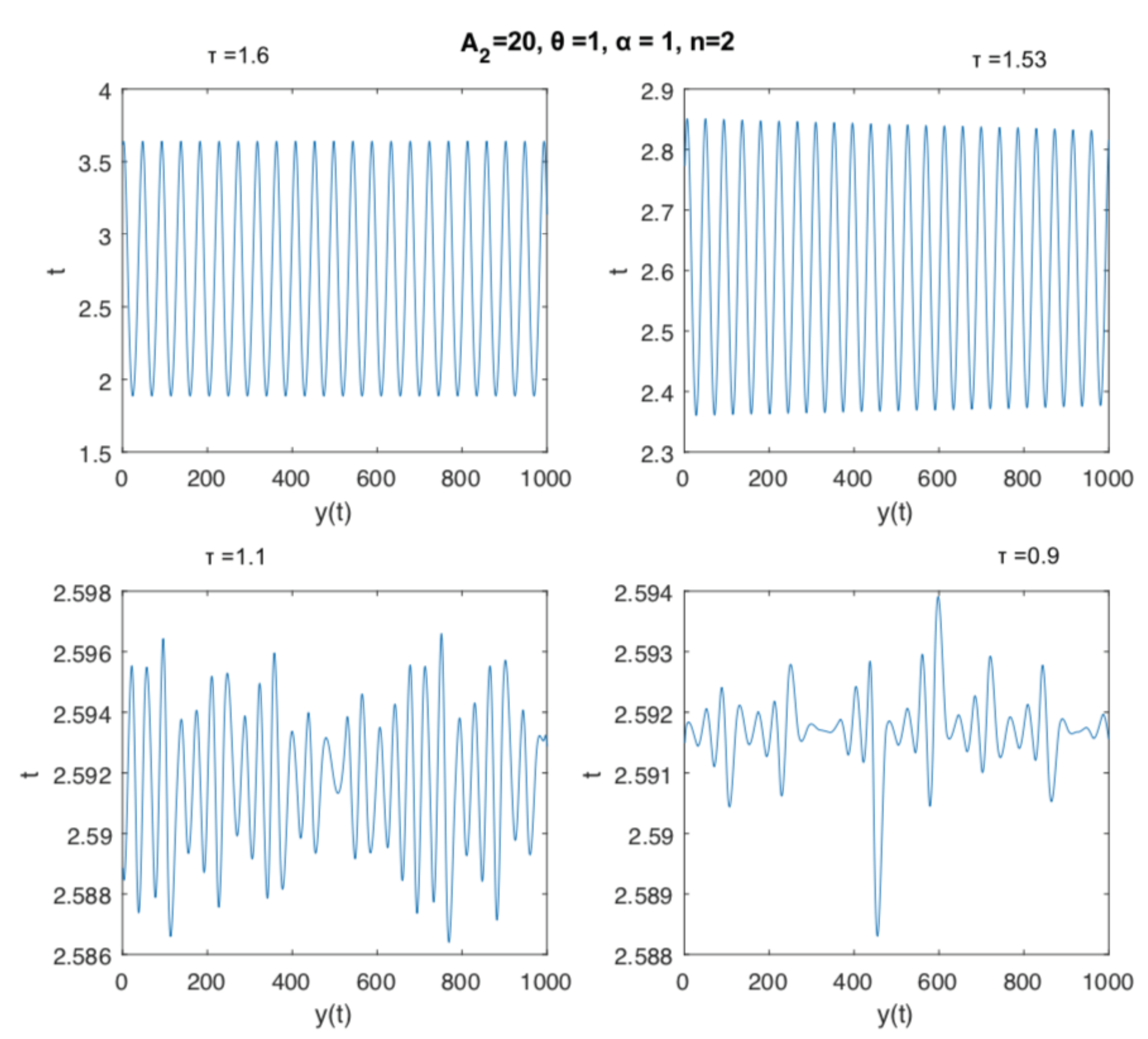
In Figure 2 we can observe the time series associated with the dynamics presented in Figure 1. Cyclic oscillations with low and high periods and irregular dynamics are typical for the values of the delay parameter shown.

Now let us consider a second case for discussion and illustration of the possible dynamics of the DDE presented in Equation (6). Let us again fix parameters $A_2=20$, $\alpha =1$, $\theta =1,\xi =\tau =1$ and let n vary from 1 to 10. For very small n (close to 1) we have a stable cycle. By increasing n, we obtain numerically that for a value between $n=1.108$ and $n=1.10836$ a bifurcation will occur, where the existing stable cycle doubles period and loss stability. Increasing values of n, more period doubling can be observed, until for $n=2.4$, we have complex oscillations (Figure 3). It is interesting to comment that very similar dynamics and patterns can be observed in both cases: stable cycle, unstable cycle, and periodic and aperiodic oscillations. The parameter n has a larger interval of variation, being the power term in a rational function; to increase the n value implies a less impact on the pupil area. In turn, the parameter $tau$ varies in a real range with less amplitude, therefore being the control parameter. In an analogy with ocular dynamics, the control parameter $tau$ should not be characterized by very high amplitude, since philologically the decrease and increase of the pupil area are highly sensitive, and large control parameters can damage the natural reactions in the dynamics of the pupil process.

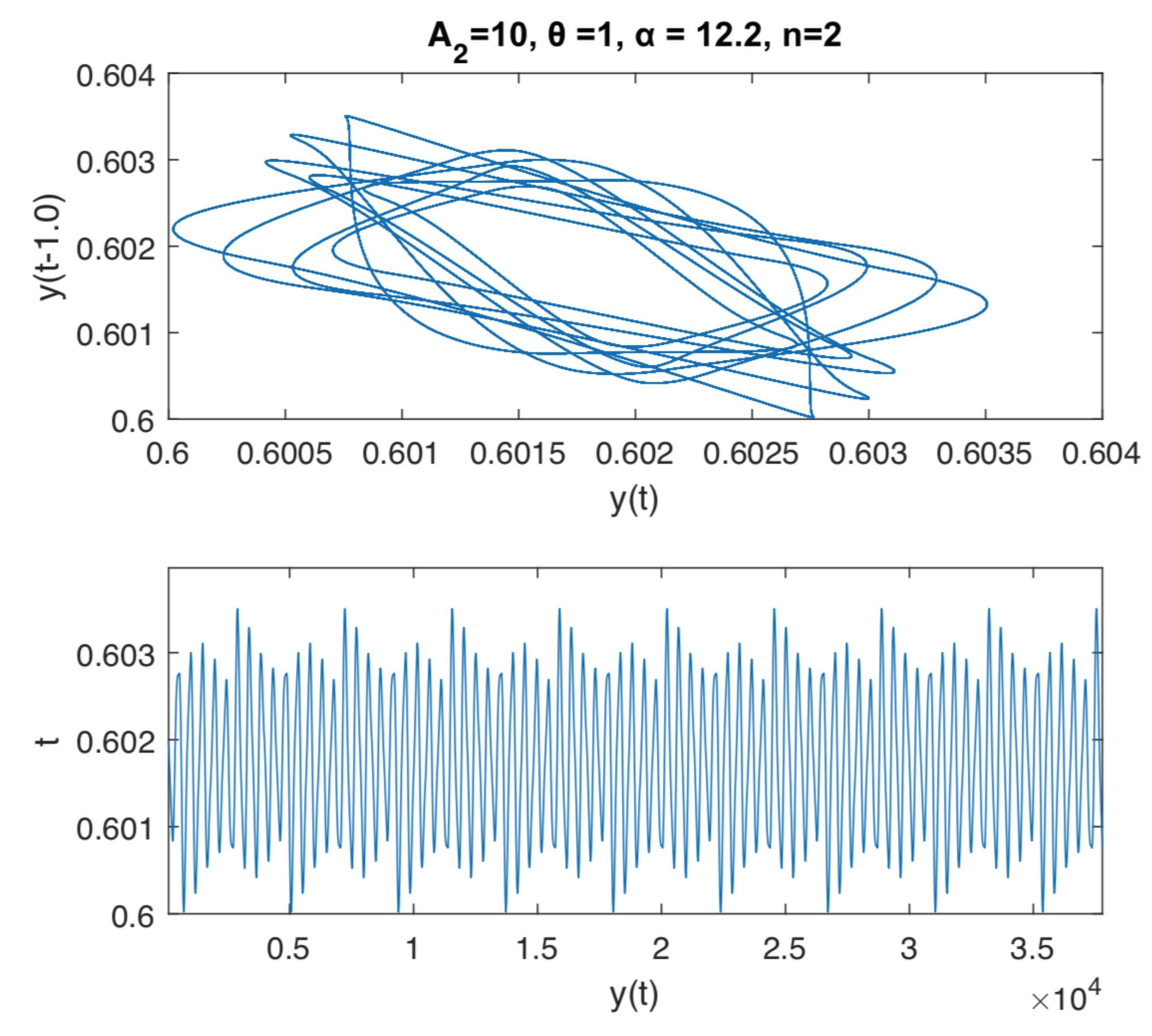
The last Figure 4 and Figure 5 are illustrating a further analysis of the rich dynamics of the considered delay differential equation. In this case we fix the delay to $\tau =1$, $\theta =1$, $n=2$, $A_2=10$ and let the parameter $\alpha$ to vary between 1 and 15. We numerically observe a pattern in the dynamics, given by a stable period 1-cycle, which loose stability, when $\alpha$ increases, and later gets transformed in a stable cycle of order-k, followed by an aperiodic orbit. This pattern is repeated several times in the $\alpha$ values interval, suggesting a kind of cyclicity in the behavior of the pupil area when one parameter is varied. These phenomena can also be interpreted as the reaction to the exposition to some kind of noise in the dynamics of the iris muscle activity in the vicinity of a Hopf bifurcation. This can be possible, because the pupil determines some kind of oscillations known as pupillary hippus. For instance, we can not explain exactly why and how this noise appears, but incorporating noise into the model can produce oscillations that are quite similar to those.

According to the numerical simulations illustrated in Figure 4 and Figure 5, the have the following conclusions: the systems asymptotically settle down to a cycle of order 18, for $\alpha =12.2,$ and to an aperiodic cycle for $\alpha =13.7$. We use a 100.000 and 200.000 time span in the interval of integration in dde23 Matlab delay differential equation with constant delay solver, in order to guarantee the stability of the attractor.

7. Conclusions

This study shows that a simple nonlinear DDE can lead to stable limit cycles and unstable complex oscillations with the variation of the parameters. Interesting results are obtained when is varied the time delay parameter. Namely, for small values of the time delay, we obtain stable limit cycles; by increasing the value of time delay parameter, we obtain bifurcations, several period cycles, and complex oscillations. After a certain value of the time delay parameter, we return to a limit cycle, which will remain stable for higher delays.

Human PRL can be modeled in two steps: the perception phase and, after some control, the adjustment phase. The way was described, the retinal light flux reaching the retina is converted into neural action potentials per unit of time and is sending as an afferent neural signal to the midbrain; after an efferent neural signal is returned, reducing or increasing the pupil size. This process justifies the adequacy of the use of a model translated by a DDE.

A deeper analysis can be done by visualizing the bifurcation diagram in one and two parameters. Further research can compare empirical data with model dynamics. We intend to work in this comparison by taking advantage of the involvement of researchers in the area of mathematics as well as in the field of ophthalmology.

References

- Baker, C.T.H.; Paul, C.A.H.; Will, D.R. A Bibliography on the Numerical Solution of Delay Differential Equations; Numerical Analysis Report 269; Mathematics Department, University of Manchester: Manchester, UK, 1995; pp. 1360–1725. [Google Scholar]
- Erneux, T. Applied Delay Differential Equations; Springer: Berlin/Heidelberg, Gernamy, 2009; Volume 3, ISBN 978-3-642-02328-6. [Google Scholar]
- Huanga, J.; Zou, X. Traveling wavefronts in diffusive and cooperative Lotka-Volterra system with delays. J. Math. Anal. Appl. 2002, 271, 455–466. [Google Scholar] [CrossRef] [Green Version]
- Faria, T.; Trofimchuk, S. Nonmonotone travelling waves in a single species reaction-diffusion equation with delay. J. Differ. Equ. 2006, 228, 357–376. [Google Scholar] [CrossRef] [Green Version]
- Epstein, R. Differential delay equations in chemical kinetics: Some simple linear model systems. J. Chem. Phys. 1990, 92, 1702–1711. [Google Scholar] [CrossRef]
- Keane, A.; Krauskopf, B.; Postlethwaite, C.M. Climate models with delay differential equations. Chaos 2017, 27, 114309–114315. [Google Scholar] [CrossRef] [PubMed]
- Bodnar, M.; Forys, U. Three types of simple dde’s describing tumor growth. J. Biol. Syst. 2007, 15, 453–471. [Google Scholar] [CrossRef]
- Atay, F.M. Delay-Induced Stability: From Oscillators to Networks. In Complex Time-Delay Systems, Theory and Applications; Atay, F.M., Ed.; Springer: Berlin/Heidelberg, Gernamy, 2010; pp. 45–62. ISBN 978-3-642-02328-6. [Google Scholar]
- Longtin, A.; Milton, J.G. Modelling autonomous oscillations in the human pupil light reflex using non-linear delay-differential equations. Bull. Math. Bio. 1989, 51, 605–624. [Google Scholar] [CrossRef]
- Moon, P.; Spencer, D. On the stiles-crawford effect. J. Opt. Soc. Am. 1979, 34, 319–329. [Google Scholar] [CrossRef]
- De Groot, S.G.; Gebhard, J.W. Pupil size as determined by adapting luminancet. J. Opt. Soc. Am. 1952, 42, 492–495. [Google Scholar] [PubMed]
- Pokorny, J.; Smith, V.C. The verriest lecture. How much light reaches the retina? Colour Vis. Defic. XIII. Doc. Ophth. Proc. Ser. 1997, 59, 491–511. [Google Scholar]
- Link, N.; Stark, L. Latency of the pupillary response. IEEE Trans. Bio. Eng 1988, 35, 214–218. [Google Scholar] [CrossRef] [PubMed]
- McDougal, D.; Gamlin, P.D.R. Pupillary control pathways. In The Senses: A Comprehensive Reference; Masland, R.H., Albright, T., Eds.; Academic Press: Cambridge, MA, USA, 2008; Volume 1, pp. 521–536. [Google Scholar] [CrossRef]
- Napieralski, P.; Rynkiewicz, F. Modeling Human Pupil Dilation to Decouple the Pupillary Light Reflex. Open Phys. 2019, 17, 458–467. [Google Scholar] [CrossRef]
- Tilmant, C.; Gindre, G.; Sarry, L.; Boire, J.-Y. Monitoring and modeling of pupillary dynamics. In Proceedings of the 25th Annual International Conference of the IEEE Engineering in Medicine and Biology Society (IEEE Cat. No.03CH37439), Cancun, Mexico, 17–21 September 2003; Volume 1, pp. 678–681. [Google Scholar] [CrossRef]
- Pamplona, V.; Oliveira, M.; Baranoski, V. Photorealistic Models for Pupil Light Reflex and Iridal Pattern Deformation. ACM Trans. Graph. 2009, 4. [Google Scholar] [CrossRef]
- Adhikari, P.; Feigl, B.; Zele, A.J. The flicker Pupil Light Response (fPLR). Transl. Vis. Sci. Technol. 2019, 8, 681–691. [Google Scholar] [CrossRef] [PubMed]
- Roussel, M. Nonlinear Dynamics Hands-On Introductory Survey; Morgan & Claypool Publishers: San Rafael, CA, USA, 2019; pp. 45–62. ISBN 978-1-64327-461-4. [Google Scholar] [CrossRef]
- Januário, C.; Grácio, C.; Mendes, D.; Duarte, J. Measuring and controlling the chaotic motion of profits. Int. J. Bifurc. Chaos Appl. Sci. Eng. 2009, 11, 3593–3604. [Google Scholar] [CrossRef]
- Taylor, S.R.; Campbell, S.A. Approximating chaotic saddles for delay differential equations. Phys. Rev. E 2007, 75, 366–393. [Google Scholar] [CrossRef] [PubMed] [Green Version]
- Szczelina, R.; Zgliczy, P.K. Algorithm for Rigorous Integration of Delay Differential Equations and the Computer-Assisted Proof of Periodic Orbits in the Mackey-Glass Equation. Found Comput. Math. 2018, 18, 1299–1332. [Google Scholar] [CrossRef] [Green Version]
- Farmer, J.D. Chaotic attractors of an infinite-dimensional dynamical system. Phys. D 1982, 4, 366–393. [Google Scholar] [CrossRef]
- Stark, L. Oscillation and Noise in the Human Pupil Servomechanism. Proc. IRE 1959, 47, 1925–1939. [Google Scholar] [CrossRef]
Figure 1.
Dynamics of Equation (5) with fixed , , and , and varying the time delay parameter in the interval , namely , , , and .
Figure 2.
Time series illustrating the dynamics of Equation (5) with fixed , , and , and varying the time delay parameter in the interval , namely , , , and .
Figure 3.
Dynamics of Equation (5) with fixed , , and varying the value of parameter n in the interval , namely , , , and .
Figure 4.
Dynamics and time series of Equation (5) with , , , and . For we can find a cycle of order 18.
Figure 5.
Dynamics and time series of Equation (5) with , , , and . For we can find a cycle of order 18. For we can find an aperiodic cycle.
© 2020 by the authors. Licensee MDPI, Basel, Switzerland. This article is an open access article distributed under the terms and conditions of the Creative Commons Attribution (CC BY) license (http://creativecommons.org/licenses/by/4.0/).
Share and Cite
MDPI and ACS Style
Laureano, R.D.; Mendes, D.; Grácio, C.; Laureano, F. Searching for Complexity in the Human Pupillary Light Reflex. Mathematics 2020, 8, 394. https://doi.org/10.3390/math8030394
AMA Style
Laureano RD, Mendes D, Grácio C, Laureano F. Searching for Complexity in the Human Pupillary Light Reflex. Mathematics. 2020; 8(3):394. https://doi.org/10.3390/math8030394
Chicago/Turabian StyleLaureano, Rosário D., Diana Mendes, Clara Grácio, and Fátima Laureano. 2020. "Searching for Complexity in the Human Pupillary Light Reflex" Mathematics 8, no. 3: 394. https://doi.org/10.3390/math8030394
Note that from the first issue of 2016, this journal uses article numbers instead of page numbers. See further details here.