A Hybrid k-Means Cuckoo Search Algorithm Applied to the Counterfort Retaining Walls Problem


1
Escuela de Ingeniería en Construcción, Pontificia Universidad Católica de Valparaíso, Valparaíso 2362807, Chile
2
Institute of Concrete Science and Technology (ICITECH), Universitat Politècnica de València, 46022 València, Spain
*
Author to whom correspondence should be addressed.
†
These authors contributed equally to this work.
Mathematics 2020, 8(4), 555; https://doi.org/10.3390/math8040555
Submission received: 16 March 2020
/
Revised: 1 April 2020
/
Accepted: 3 April 2020
/
Published: 10 April 2020
(This article belongs to the Special Issue Optimization for Decision Making II)
Abstract
:The counterfort retaining wall is one of the most frequent structures used in civil engineering. In this structure, optimization of cost and CO2 emissions are important. The first is relevant in the competitiveness and efficiency of the company, the second in environmental impact. From the point of view of computational complexity, the problem is challenging due to the large number of possible combinations in the solution space. In this article, a k-means cuckoo search hybrid algorithm is proposed where the cuckoo search metaheuristic is used as an optimization mechanism in continuous spaces and the unsupervised k-means learning technique to discretize the solutions. A random operator is designed to determine the contribution of the k-means operator in the optimization process. The best values, the averages, and the interquartile ranges of the obtained distributions are compared. The hybrid algorithm was later compared to a version of harmony search that also solved the problem. The results show that the k-mean operator contributes significantly to the quality of the solutions and that our algorithm is highly competitive, surpassing the results obtained by harmony search.
1. Introduction
Combinatorial optimization problems appear naturally in the areas of engineering and science. From the research point of view, these problems present interesting challenges in the areas of operations research, computational complexity, and algorithm theory. Examples of combinatorial problems are found in, scheduling problems [1,2], transport [2], machine learning [3], facility layout design [4], logistics [5], allocation resources [6,7], routing problems [8,9], robotics applications [10], civil engineering problem [11,12,13], engineering design problem [14], fault diagnosis of machinery [15], and social sustainability of infrastructure projects [16], among others. Combinatorial optimization algorithms should explore the solutions space to find optimal solutions. When the space is large, this cannot be fully explored. Combinatorial optimization algorithms address this difficulty, reducing the effective space size, and exploring the search space efficiently. Among these algorithms, metaheuristics have been a good approximation to obtain adequate solutions. However, addressing large instances and requiring almost real-time solutions for some cases, motivates lines of research that strengthen the methods that address these problems.
One way to classify metaheuristics is according to the search space in which they work. In that sense, we have metaheuristics that work in continuous spaces, discrete and mixed spaces [17]. An important line of inspiration for metaheuristic algorithms are natural phenomena, many of which develop in a continuous space. Examples of metaheuristics inspired by natural phenomena in continuous spaces are: Optimization of particle swarm [18], black hole [19], cuckoo search (CS) [20], Bat algorithm [21], Algorithm of fire fly [22], fruit fly [23], artificial fish swarm [24], gravitational search algorithm [25], among others. The design of discrete versions of these algorithms carries important challenges because they must try to preserve the intensification and diversification properties [17].
With the aim of modifying and improving the results of a metaheuristic algorithm, the main tool available to them is tuning their control parameters. These types of modifications correspond to small modifications of the algorithm since the operating mechanism of the algorithm is not altered. However, many optimization problems cannot be efficiently addressed by an algorithm through modification of its parameters and require deep modifications that alter its mechanism of operation [17,26]. A strategy that has strengthened the results of metaheuristic algorithms has been the hybridization of these with techniques that come from the same and the other areas. Hybridization strategies involve deep changes to the original algorithm. The main hybridization proposals found in the literature are the following: (i) matheuristics, where mathematical programming is combined with metaheuristic techniques [27], (ii) hybrid heuristics, hybridization between different metaheuristic methods [28], (iii) simheuristics, that combine simulation and metaheuristics [29], and (iv) the hybridization between machine learning and metaheuristics. The latest line of research exploring the integration between the areas of machine-learning and metaheuristic algorithms is an emerging line of research in the areas of computing, mathematics, and operational research. In developing the state-of-the-art, we find that hybridization occurs primarily for two purposes. The first, with the goal that metaheuristics help machine-learning algorithms improve their results (for example, [30,31]). In the second intention, machine-learning techniques are used to strengthen metaheuristic algorithms (for example, [32,33]). The details of the hybridization forms are specified in Section 2.
In this article, inspired by the research lines mentioned above. A hybrid algorithm is designed, which explores the application of a machine-learning algorithm in a discrete operator to allow continuous metaheuristics to address combinatorial optimization problems. We will apply our hybrid algorithm to the discrete problem of the design of counterfort retaining walls. The contributions of this work are detailed below:
- A machine-learning algorithm is proposed to allow metaheuristics commonly defined and used in continuous optimization addressing discrete optimization problems simply and effectively. To perform this process, the algorithm uses k-means. This clustering technique has been selected because it has solved other binary combinatorial problems efficiently [5,33]. The selected metaheuristic is CS. Its selection is because it has been frequently used in solving continuous optimization problems and its tuning is relatively simple, which allows focusing on the discretization process.
- A random operator is designed to study the contribution of the k-means operator in the discretization process.
- This hybrid algorithm is applied to the design of the buttresses retaining wall problem. Optimization is carried out for cost and emissions of CO2. A comparison is made between the proposed hybrid algorithm and an adaptation of the harmony search (HS) proposed in [34]. The design of the counterfort retaining walls will be detailed in Section 3.
The structure of the remaining of the paper is as follows: a state-of-the-art of hybridizing metaheuristics with machine learning is developed in Section 2. In Section 3 the optimization problem, the variables involved, and the restrictions are defined. The discrete k-means algorithm is detailed in Section 4. The experiments and results obtained are shown in Section 5. Finally, in Section 6 the conclusions and new lines of research are summarized.
2. Hybridizing Metaheuristics with Machine Learning
Metaheuristics form a wide family of algorithms. These algorithms are classified as incomplete optimization techniques and are usually inspired by natural or social phenomena [17,35]. The main objective of these is to solve problems of high computational complexity and they own the property of not having to deeply alter their optimization mechanism when the problem to be solved is modified. On the other hand, machine-learning techniques correspond to algorithms capable of learning from a dataset [36]. If we make a classification according to the way of learning, there are three main categories: Supervised learning, unsupervised learning, and learning by reinforcement. Usually, these algorithms are used in problems of regression, classification, transformation, dimensionality reduction, time series, anomaly detection, and computational vision, among others.
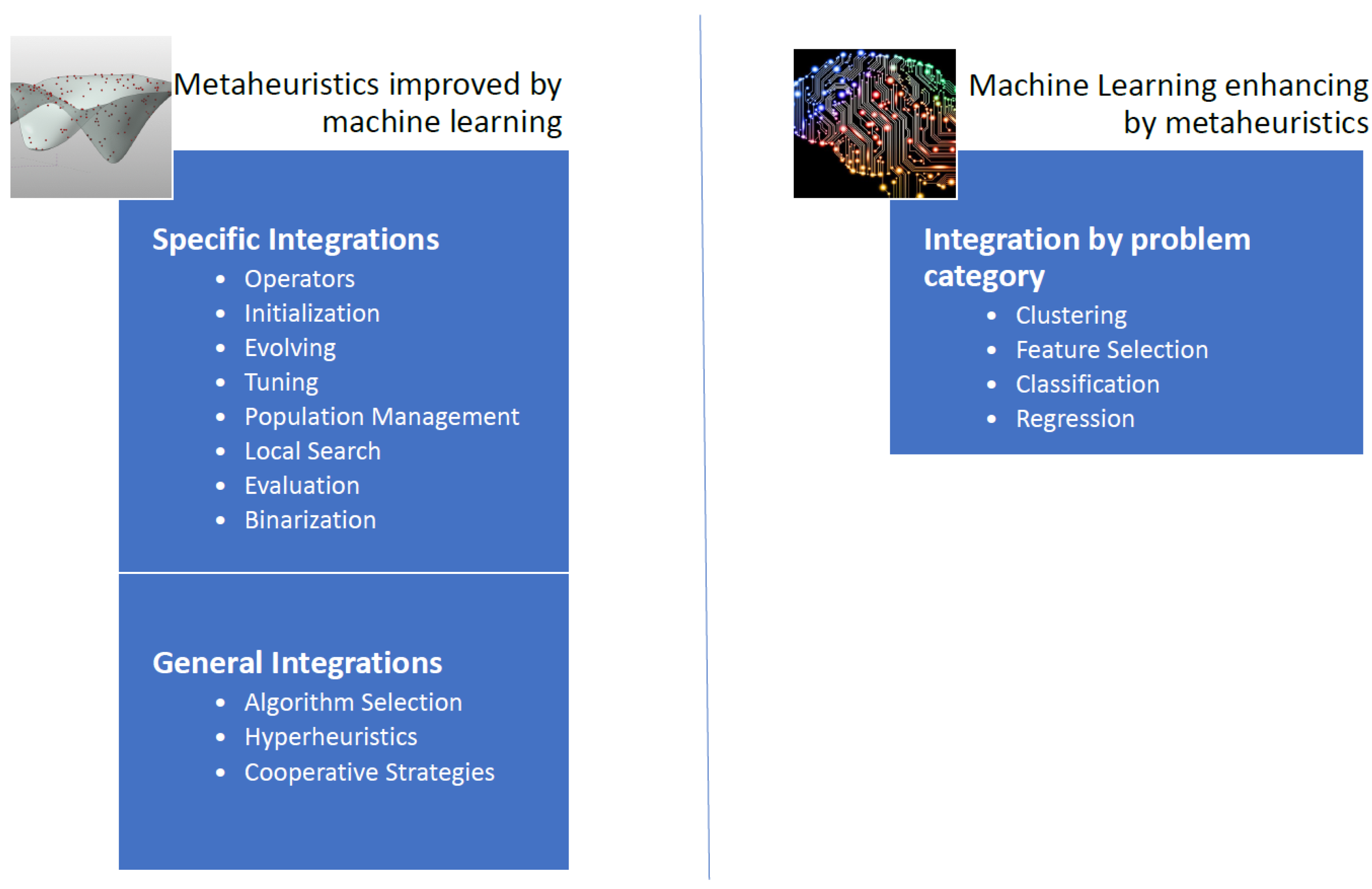
In the state-of-the-art of algorithms that integrate machine-learning techniques with metaheuristic algorithms, we have found two main approaches [26]. In the first approach, machine-learning techniques are used in order to improve the quality of the solutions and convergence rates obtained by the metaheuristic algorithms. The second approach uses metaheuristic algorithms to improve the performance of machine-learning techniques [26]. Usually, the metaheuristic is responsible for solving more efficiently an optimization problem related to the machine-learning technique. Adapted and extended from [26], in Figure 1, we have proposed a general scheme of techniques where machine learning and metaheuristics are combined.
When we analyze the integration mechanisms of the first approach, we identify two lines of research. In the first line, machine-learning techniques are used as metamodels in order to select different metaheuristics, therein choosing the most appropriate for each instance. The second line aims to use specific operators that make use of machine-learning algorithms and subsequently this specific operator is integrated into a metaheuristic [26].
In the general integration of machine-learning algorithms on metaheuristic techniques we find three main groups: algorithm selection, hyper-heuristics, and cooperative strategies. In algorithm selection, the goal is to choose from a set of algorithms and considering the associated characteristics for each instance of the problem, an algorithm that works best for similar instances. Another way to approach the problem is to automate the design of heuristic or metaheuristic methods to tackle a wide range of problems, we call this hyperheuristic approximation. Finally, the objective of cooperative strategies is to mix algorithms in a parallel or sequential way to obtain more robust methods. The cooperation mechanism can be complete, i.e., sharing the complete solution, or partial when only part of the solution is shared. In [32], the problem of docking scheduling in massive terminals was addressed by algorithm selection techniques. In [37], the nurse training problem through a tensor-based hyperheuristic algorithm was addressed. Finally, a distributed framework that uses agents was proposed in [38]. In this framework, each agent corresponds to a metaheuristic and the framework can adapt through direct cooperation. This framework was applied to the problem of permutation flow stores.
Additionally, a metaheuristic incorporates operators that allow strengthening its performance. Examples of these operators are initialization operators, solution perturbation, population management, binarization, parameter configuration, and local search operators, among others [26]. Specific integrations explore the machine-learning application in some of these operators [26]. In the design of binary versions of algorithms that work naturally in continuous spaces, we find binarization operators in [2]. These binary operators use unsupervised learning techniques to perform the binarization process. In [39], the concept of percentile was explored in the process of generating binary algorithms. In addition, in [1], the Apache spark big data framework was applied to manage the population size of solutions to improve convergence times and the quality of results. Another interesting research line was found in the adjustment of metaheuristic parameters. In [40], the parameter setting of a chess classification system was implemented. Based on decision trees, and using fuzzy logic, a semi-automatic parameter setting algorithm was designed in [41]. Usually, in the initiation of solutions, a random mechanism is used. However, using machine-learning techniques, algorithms have been developed that improve the initiation stage of a solution. Applied to the problem of designing a weighted circle in [42], a case-based reasoning technique was used to start a genetic algorithm. In [43] Hopfield neural networks were applied to initiate solutions of a genetic algorithm. This initiation was applied to an economic dispatch problem.
To improve the quality of machine-learning algorithms, we see that metaheuristics have a broad contribution. Contributions are found in problems of feature selection, classification, clustering, extraction of characteristics, among others. In the identification of breast cancer, in [44] a genetic algorithm was designed that improves the performance of support vector machine (SVM) when applied in image analysis. The genetic algorithm was used in the characteristic extraction stage from the images. In [45] a multiverse algorithm was used to adjust the parameters of an SVM classifier. An improved monarch butterfly algorithm was used in [46] with the goal to optimize the weights of a feed-forward neural network. In [47], a geotechnical problem was addressed. In this article, a firefly algorithm was integrated with the least-squares support vector machine technique. When considering regression problems, there are again several cases where metaheuristics have contributed. For example, in predicting the strength of high-performance concrete, in [48] a metaheuristic was used to improve the least-squares technique. In [49], share price prediction was improved by integrating metaheuristics into a neural network. Again, in the prediction of the share price of construction companies in Taiwan, in [30], a sliding-window metaheuristic-optimized machine-learning algorithm was designed, which integrates a metaheuristic in its learning process. Optimization of the parameters of a least-squares regression was improved, in [50] using a firefly algorithm. We also found metaheuristic applications for unsupervised learning techniques. In particular, there are significant contributions from metaheuristics to clustering techniques. For example, in [51], we found an algorithm application that integrates a metaheuristic with a kernel intuitionistic fuzzy c-means. This algorithm was applied to different data sets. Another integration found for clustering techniques is the search for centroids. This problem is to find the set of centroids that best group the data under a certain metric. This is an NP-hard type problem and therefore it is natural to approach it with a metaheuristic. In [52] an algorithm was proposed that uses a bee colony to solve a problem of grouping energy efficiency data obtained from a wireless sensor network. In [53], a metaheuristic was used to find centroids in planning the transportation of employees from an oil platform via helicopters. In the case of neural networks, metaheuristics have contributed to different types of integration. In [54] a metaheuristic algorithm is used to automatically find the appropriate number of neurons in a feed-forward neural network. In [55] a metaheuristic algorithm allows determining the dropout probability in convolutional neural networks. The cuckoo search and bat algorithm algorithms were used in [56] to adjust the weights of neural networks of feed-forward type. In [57] an algorithm was designed using metaheuristics to optimize convolutional neural networks. An application to long term short memory (LSTM) neural network training was studied in [58]. LSTM networks were applied in healthcare analysis.
Inspired by the lines of research detailed above, this work proposes a hybrid algorithm in which the unsupervised k-means learning technique is used to obtain binary versions of the cuckoo search optimization algorithm. This hybrid algorithm was used to solve the problem of the counterfort retaining walls. The k-means technique has been widely used and in recent studies, it has been applied in [59] to bioinformatics for detecting gene expression profile, image segmentation for pest detection [60] in agriculture, and brain tumor identification [61], among others. Particularly the k-means technique has been previously applied in obtaining binary versions of continuous metaheuristics and used to solve the multidimensional knapsack problem [33] and the set covering problem [5] which are NP-hard problems. In the case of the cuckoo search, hybrid versions of this algorithm have been applied in [62] to numerical optimization problems in engineering. In [63] cuckoo search was applied to benchmark functions and engineering design problems. An algorithm with reinforced learning was used in [64] to solve a logistic distribution problem. In [65] an improved version of the cuckoo search was applied to drone location.
3. Problem Definition
In this Section, we will detail the buttressed earth-retaining walls optimization problem. In Section 3.1 we will give the definition of the optimization problem. Later in Section 3.2, we will detail the design variables. Then the design parameters will be described in Section 3.3, and finally, in Section 3.4, we define the constraints.
3.1. Optimization Problem
The optimization problem considers two objective functions, which will be addressed independently. The first function corresponds to the cost () of the wall construction, expressed in euros. The second one considers the CO2 equivalent emissions units (). These construction units correspond to formwork, materials, excavation and earth-fill. The cost and emission functions are based on a 1 m wide strip [34]. The emission and cost values were obtained from [34,66] and are shown in Table 1. Then, in a general way, our optimization problem is defined according to Equation (1).
where x is the set of decision variables and , corresponds to cost or emissions. Additionally, the optimization problem is subject to a set of restrictions determined by the ultimate (ULS) and service (SLS) state limits.
3.2. Problem Design Variables
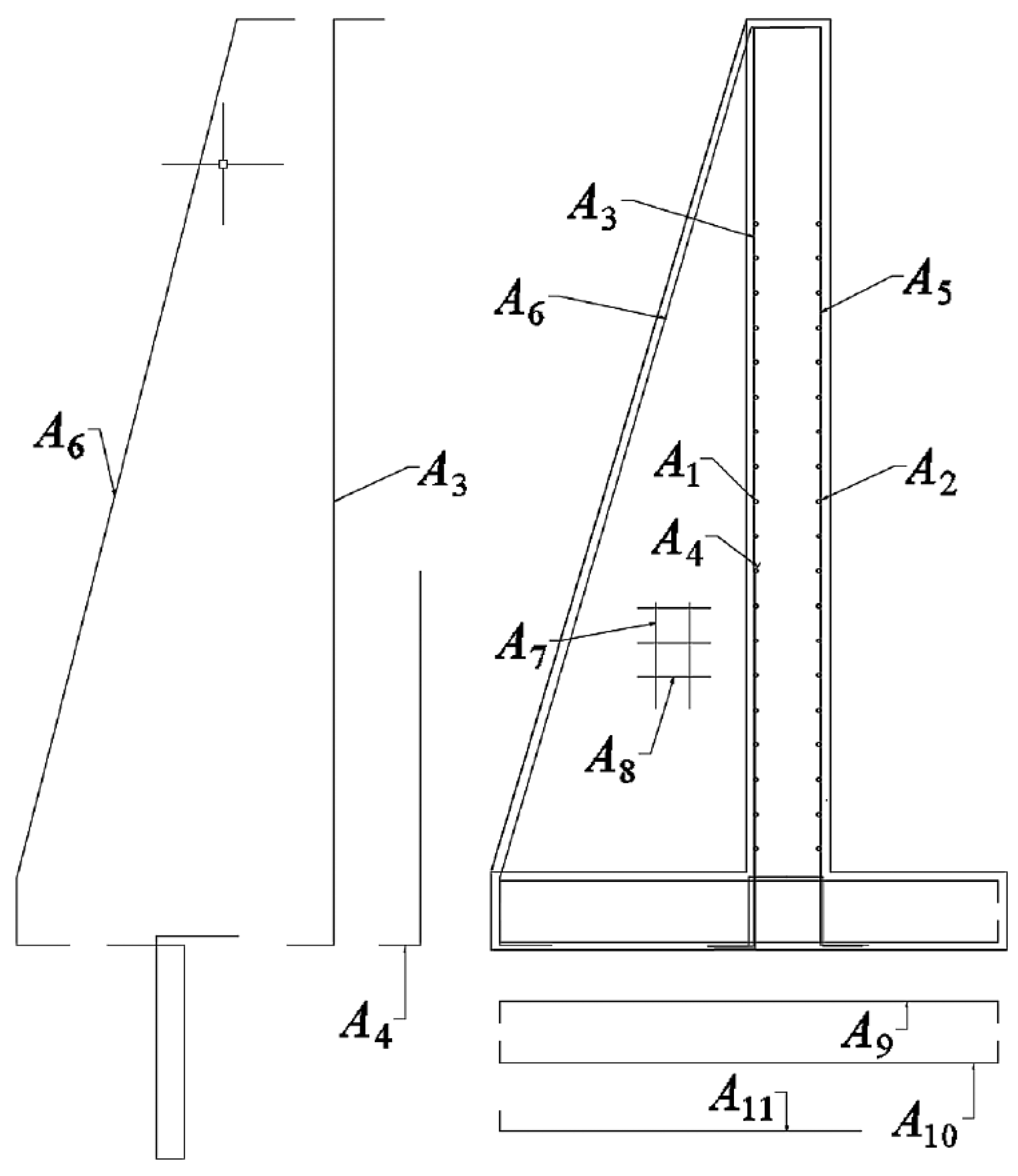
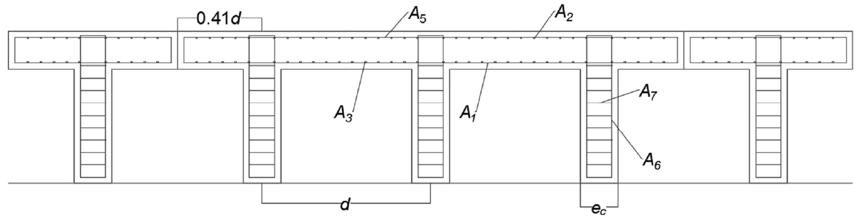
In the design of the buttressed retaining wall to study, three groups of variables are defined. The geometric variables, the concrete and steel grade, and the passive reinforcement of the wall. In total there are 32 variables where each of these has a discrete amount of possibilities. In the group of concrete and steel grades. Concrete HA-25 to HA-50 is considered in discrete intervals of 5 MPa. In the case of steel, the B500S and B400S types are considered. In the group of geometric variables, there is the thickness of the footing (c), thickness of the stem (b), the length of the toe (p), the thickness of the buttresses (), the length of the heel (t) and the distance between buttresses (d). The last group of variables that correspond to the passive reinforcement of the wall. There are 24 variables shown in Figure 2 and Figure 3. The diameter and the number of bars define the reinforcement. Three reinforcement flexural bars defined as A1, A2 and A3 contribute in the main bending of the stem. The vertical reinforcement of foundation in the rear side of the stem is given by A4, up to a height L1. The secondary longitudinal reinforcement is given by A5 for shrinkage and thermal effects in the stem. The longitudinal reinforcement of the buttress is given by A6. The area of reinforcement bracket from the bottom of the buttress is given by A7 and A8. The upper and bottom heel reinforcement are defined by A9 and A11 and the shear reinforcement in the footing by A12. The longitudinal effects in the toe are defined by A10. The set of combinations of the values for the 32 variables shown in Table 2, constitutes the solution space.
3.3. Problem Design Parameters
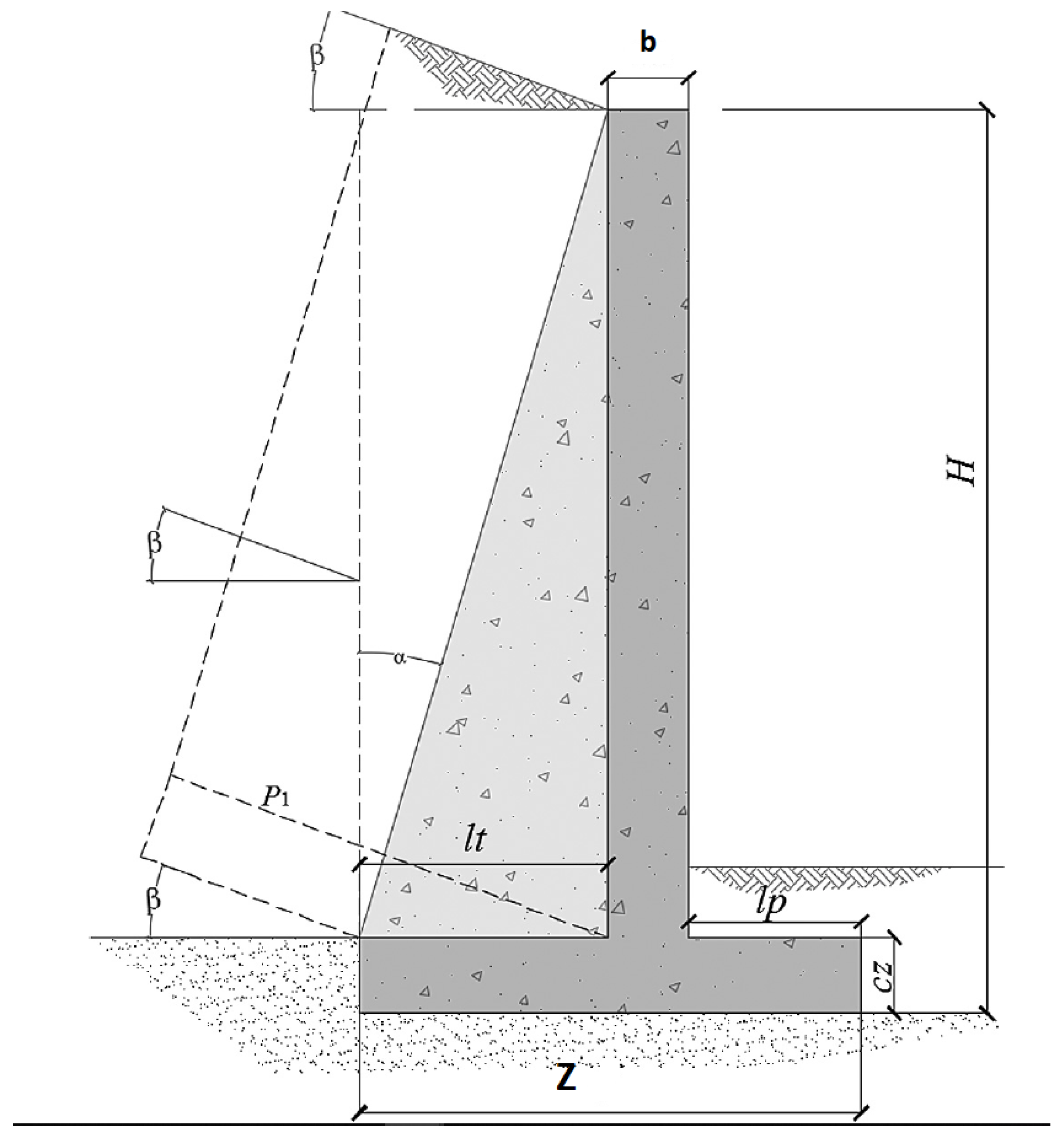
The data that will remain fixed in the optimization process will be called problem design parameters. The main design parameters are shown in Figure 4. The height of the wall and the depth of the soil in front of the wall are denoted by H and H2, respectively. The maximum bearing pressure is the soil foundation ultimate bearing capacity divided by the bearing capacity factor of safety. The maximum support pressure for the operating conditions is represented by , the base-friction coefficient is and the backfill slope at the top of the rod is . The density, the internal friction angle and the friction angle that determine the earth’s pressure angle are given respectively by P (, , ). The roughness between the wall and the fill is determined by a fraction of . The values of the problem design parameters are shown in Table 3.
3.4. Problem Constraints
The feasibility of the structure is verified in accordance with the Spanish technical standards defined in [68] and the recommendations detailed in [69]. The flexural and shear limit states are checked. The structure is verified in accordance with the approach specified in [70]. To check the structure limit states, a uniform surface load at the top of the fill is considered [71]. For the active earth pressure calculation the surface loads and fill are considered. The major forces in wall analysis consider wall weight, heel backfill load, surface load, earth pressure, weight at the front toe, and passive resistance against the toe. Buttresses receive a load equivalent the product of the distance between the buttresses by the pressure distribution in the stem.
The structural model considers that the upper part of the stem works as a cantilever, while the lower part of the stem is strongly coerced by two elements: the footing and the lower part of the buttress, located at the rear of the stem. Calculation bending moments are taken in the midsection between the buttresses and are given by and described in Equations (2) and (3) respectively.
is the bending moment at the connection of the stem to the footing, is the maximum bending moment on the stem and represents the pressure over the slab on the upper side of the footing. When the spacing of the buttresses is less than 50% of the height, Equation (4) defines the shear resistance (s) at the connection of the plate to the footing. For an accurate estimate of the moments in each section of the stem, as a result of the vertical bending stress in the stem, the trapezoidal pressure distribution is considered [70]. 50% of the maximum pressure at the top of the foundation is taken as the maximum value. Taking into account the vertical bending moment in the upper quarter part of the stem may be insignificant due to the involvement of [70].
Verification of the bending stress in the T-shaped horizontal cross-section is made considering the effective width, according to [72]. Mechanical bending and shear capacity are evaluated using the equations expressed in [71]. In this manual, the construction limit states of the EHE Structural Concrete Code are considered. The checks against sliding, overturning, and soil stresses, are carried out taking into account the effect of the buttresses, and are given in Equations (5)–(7). In the overturning check, Equation (5) ensures that the favorable overturning moments are sufficiently greater than the unfavorable overturning moments. In Equation (6), is the total favorable overturning moment. In Equation (7), is the unfavorable total overturn moment, and the overturning safety factor is and is taken as 1.8 for frequent events. Equation (8) represents the reaction of soil against sliding. As is the base-friction coefficient, corresponds to the total sum of the ground and wall weights located at the heel and toe, and determines the passive resistance against the toe defined by Equation (9).
4. The K-Means Discrete Algorithm
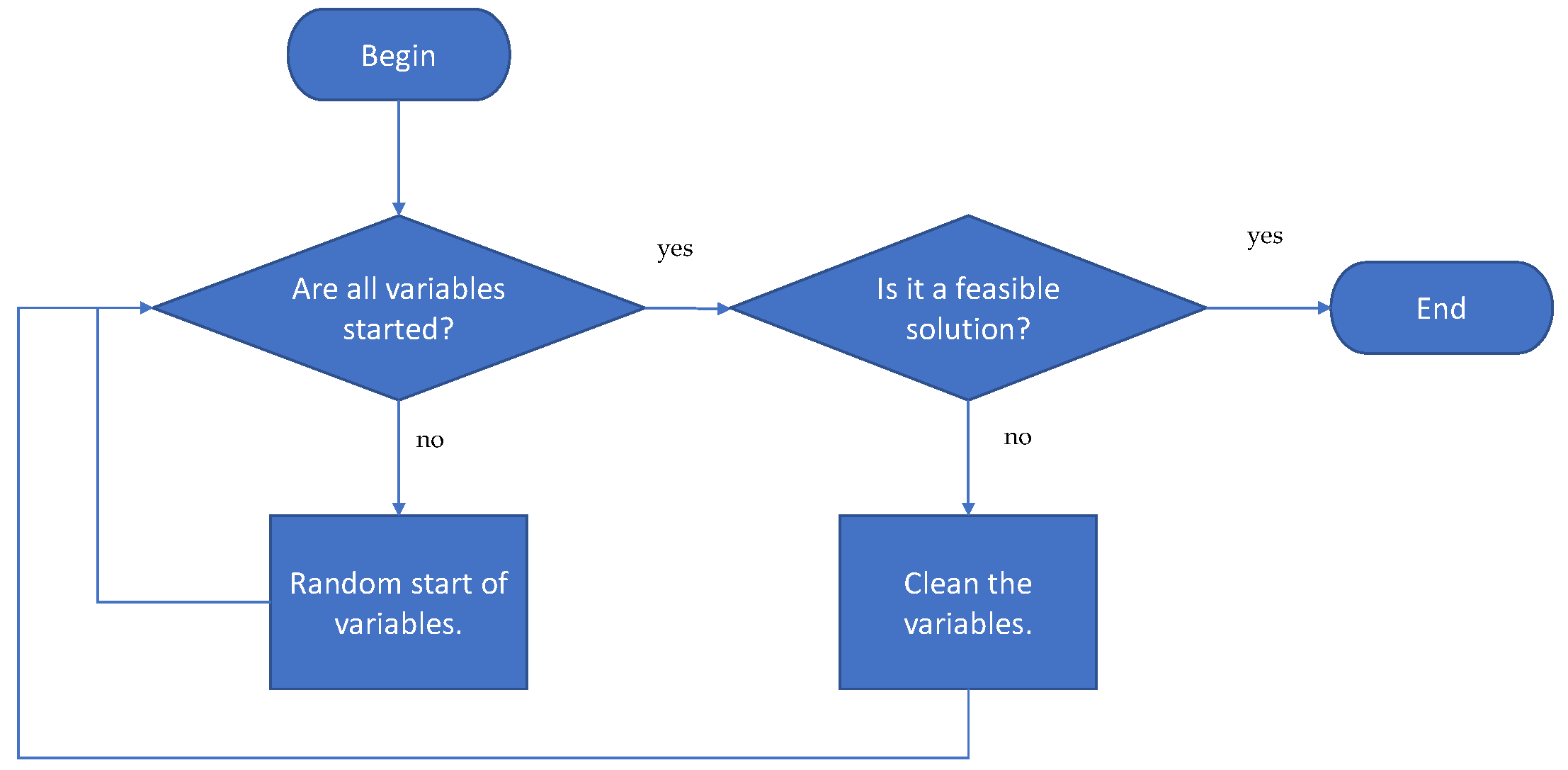
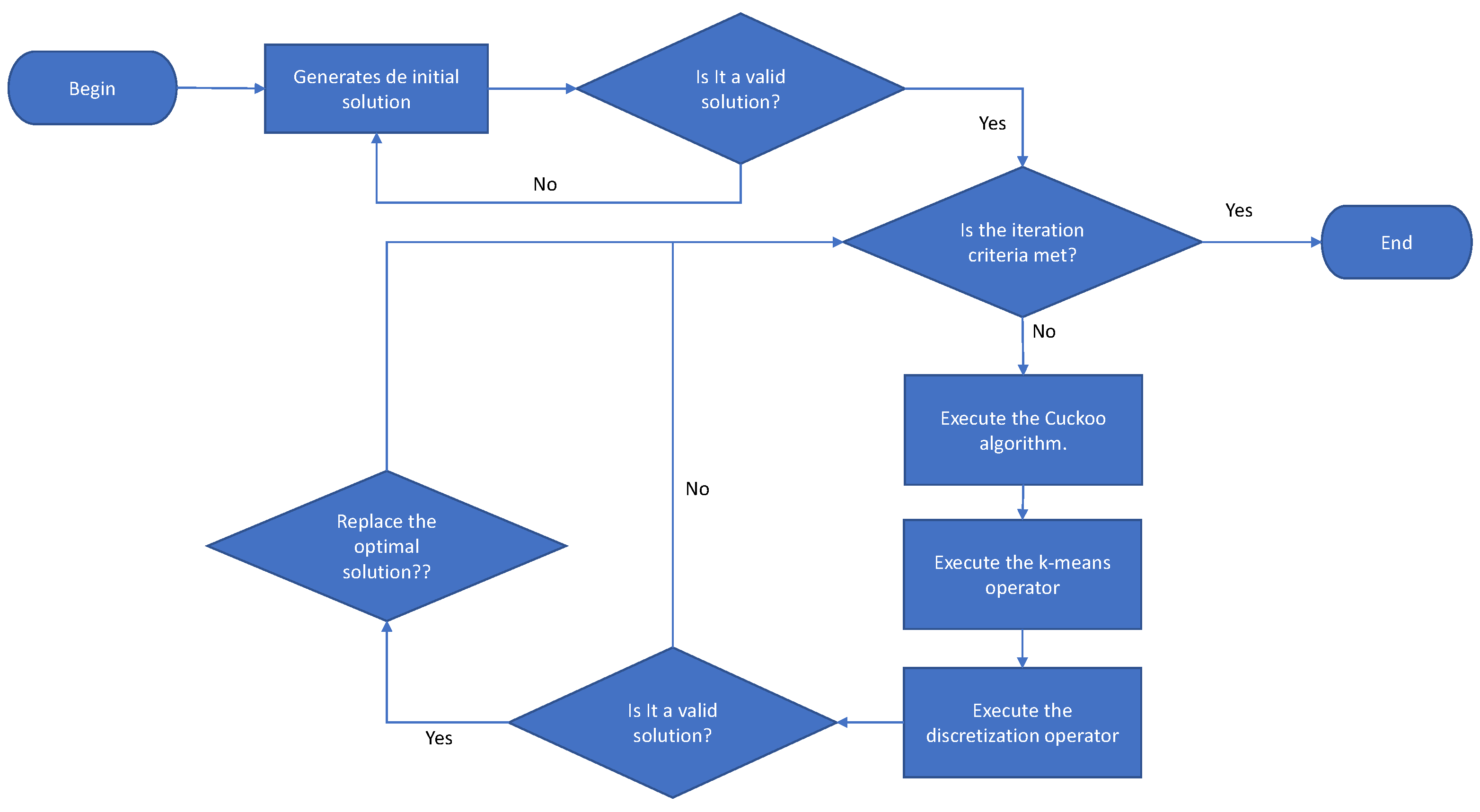
The first stage of the algorithm corresponds to generating valid solutions randomly. In the generation procedure, it is first validated if all the variables that make up the solution have been started. If not, the variables are started randomly. Once all the variables are generated, the next step is to validate if the solution obtained is feasible. In the event that it is not feasible, all the variables are cleaned, and they have generated again. The detail of the initiation procedure is shown in Figure 5. Once we have a valid set of solutions, continuous metaheuristics are used in this case CS, to produce a new solution in continuous space. The CS algorithm will be described in Section 4.1. Subsequently, we apply the k-means operator to transform continuous movements into transition probabilities. The k-means operator will be detailed in Section 4.2. The result of the transition probabilities generated by k-means are used by the discretization operator to generate a new solution. The discretization operator is detailed in Section 4.3. Finally, the new solution is validated and, in the case that it complies with the restrictions, it is compared with the best solution obtained. In the case that the new one is superior, it is replaced. The detail flow chart of the solution is shown in Figure 6.
4.1. Cuckoo Search Algorithm
The phenomenon of cuckoo species, which lay their eggs in the nests of other bird species, has inspired the CS algorithm. Such is the level of sophistication of cuckoo birds that in some cases even the colors and patterns of the eggs of the chosen host species are mimicked. In the analogy, an egg corresponds to a solution. The concept behind the analogy is to use the best solutions (cuckoos) with the aim of replacing those that do not perform well. The CS algorithm uses three basic rules:
- Each cuckoo lays one egg at a time and deposits its egg in a randomly chosen nest.
- The nests with the best results, i.e., with high-quality eggs, will be considered in the next generation.
- The number of nests available is a fixed parameter. The egg laid by a cuckoo can be discovered by the host bird with a probability
The algorithm pseudo-code is shown in Algorithm 1.
| Algorithm 1 Cuckoo search algorithm |
| 1: Objective function f(x) |
| 2: Generate initial solutions of n host nests. |
| 3: while stop criterion are meet do |
| 4: Get a cuckoo randomly and replace using Lévy flights. |
| 5: Evaluate the fitness. |
| 6: Choose in a random way a nest j among n: |
| 7: if > then |
| 8: replace the solution. |
| 9: end if |
| 10: portion of the worst nests are eliminated and new ones are created. |
| 11: keep best solutions. |
| 12: find the current best |
| 13: end while |
4.2. k-Means Operator
The goal of the k-means operator is to group the different solutions obtained by executing continuous metaheuristics in this case CS. However, this operator can be applied to any continuous swarm intelligence metaheuristics. When we consider solutions as particles, we understand the position of the particle as the location of the solution in the search space, while the velocity represents the vector of the transition of the solution from the t iteration to the iteration.
In the k-means operator (kmeanOp), the k-means clustering technique is used to make transitions in a discrete space. The proposal is based on using the movements generated by the CS metaheuristic in each dimension for all the particles. Let be a solution in iteration t, then represents the magnitude of the displacement in the i-th position, considering the iterations t and . Once all the displacements have been calculated, they are grouped using the magnitude of the displacement , we do not consider the sign. This grouping is done using the k-means technique where k represents the number of groups used. Finally, we propose a generic function shown in Equation (10) with the objective of assigning a transition probability to each displacement.
Then using the function , a probability is assigned to each group obtained from the clustering process. In this article, we use the linear function given in Equation (11). Where Clust () indicates the location of the group to which belongs. The coefficient represents the transition probability and the coefficient models the transition separation for the different groups. Both parameters must be estimated. The pseudo-code of the discretization procedure is shown in Algorithm 2.
| Algorithm 2 k-means operator |
| 1: Function kmeanOp(, ) |
| 2: Input , |
| 3: Output lTranProb(t+1) |
| 4: getDelta(, ) |
| 5: getClusters(,k) |
| 6: getTranProb(, )–Equation (11) |
| 7: return () |
4.3. Discretization Operator
As input the operator receives the transition probabilities () obtained in the previous stage and the list of solutions . For each solution , we consider each component and evaluate if it should be modified according to its transition probability. The transition probability is compared with a random number . In case the change is selected, the movement can increase the value (+1) or decrease it (−1). Finally, the selected value is compared with the best value obtained by the algorithm and remains with the minimum of both. The pseudo-code of the discrete procedure is shown in Algorithm 3.
| Algorithm 3 Discretization operator. |
| 1: Function DiscOp(, ) |
| 2: Input |
| 3: Output –Where x(t+1) is discrete. |
| 4: movement = 0 |
| 5: for do |
| 6: if then |
| 7: movement = 1 |
| 8: else |
| 9: movement = −1 |
| 10: end if |
| 11: = max(1,min(, + movement)) |
| 12: end for |
5. Results and Discussion
This Section aims to describe the results obtained by the hybrid algorithm when applying it to the counterfort retaining walls problem. In the first stage, the contribution of the k-means operator in the discretization process will be determined. This is described in Section 5.2. Later, in a second stage, we will compare our proposal with another algorithm that has solved the problem, Section 5.3. For each problem, we make 30 independent runs. The value 30 is widely accepted for statistical conclusions [73]. The Wilcoxon signed-rank [74] method was the test selected to determine if the difference is statistically significant. The p-value used was 0.05. The selection of the test is based on the methodology proposed in [73]. In this methodology, the Shapiro–Wilk or Kolmogorov—Smirnov-Lilliefors normality test is applied first. In the event that one of the populations is not normal, and both populations have the same number of points, the Wilcoxon signed-rank is suggested to verify the difference. In our case, the Wilcoxon test was applied to the entire population of instances considering all executions and comparing the results of both algorithms. For the execution of the instances, a laptop with a Core i7-4770 as a processor and 16GB in RAM has been used. The algorithm was programmed in Python 3.6.
5.1. Parameter Settings
To calibrate the parameters, heights 8 and 12 were used. These heights were selected with the intention of considering walls of different complexity. 8 represents small size walls and 12 represents larger size walls where the satisfaction of stability restrictions is much more difficult. Subsequently, each configuration was executed 5 times for each height considering all the configurations proposed in Table 4. The value 5 was chosen with the intention of being able to execute all the combinations in a limited time. In Table 4, the range column shows the scanned values to perform the CS adjustment. These ranges were inspired by previous studies in which the k-means technique was applied to solve the multidimensional knapsack problem [33] and the problem of the set covering [5]. The flow chart of the parameter settings is shown in Figure 7. For more detail on the method, reference [33] can be consulted.
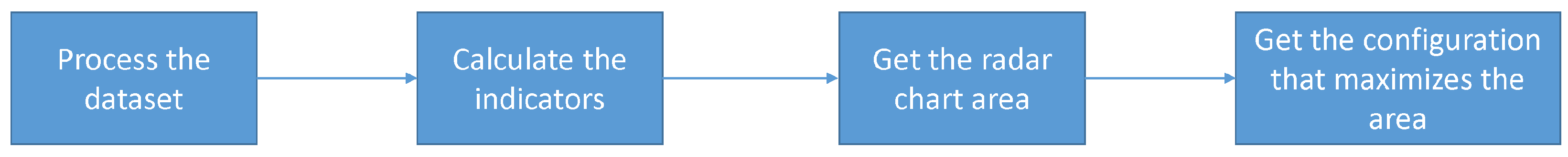
To determine the best configuration, the method proposed in [33] was used. In this method, 4 measurements are defined that I know are shown in Equations (12)–(15). The BestGlobalValue represents the best value obtained considering all the configurations. The BestLocalValue, corresponds to the best value obtained in the evaluated configuration. The minGlobalTime is the minimum convergence time considering all settings. Finally, the convergenceLocalTime represents the average convergence time for a configuration. Each of the measures defined, the closer to 1, the better performance that indicator is having. On the other hand, the closer to 0 the worse performance. Since there are 4 measurements to be able to make the evaluation, we incorporate them into a radar chart and calculate their area. As a consequence of the measurement definition, the largest area corresponds to the configuration that has the best performance considering the 4 defined measures.
- The deviation of the best local value obtained in five executions compared with the best global value:
- The deviation of the worst value obtained in five executions compared with the best global value:
- The deviation of the average value obtained in five executions compared with the best global value:
- The convergence time for the average value in each experiment is normalized according to Equation (15).
5.2. Random Operator
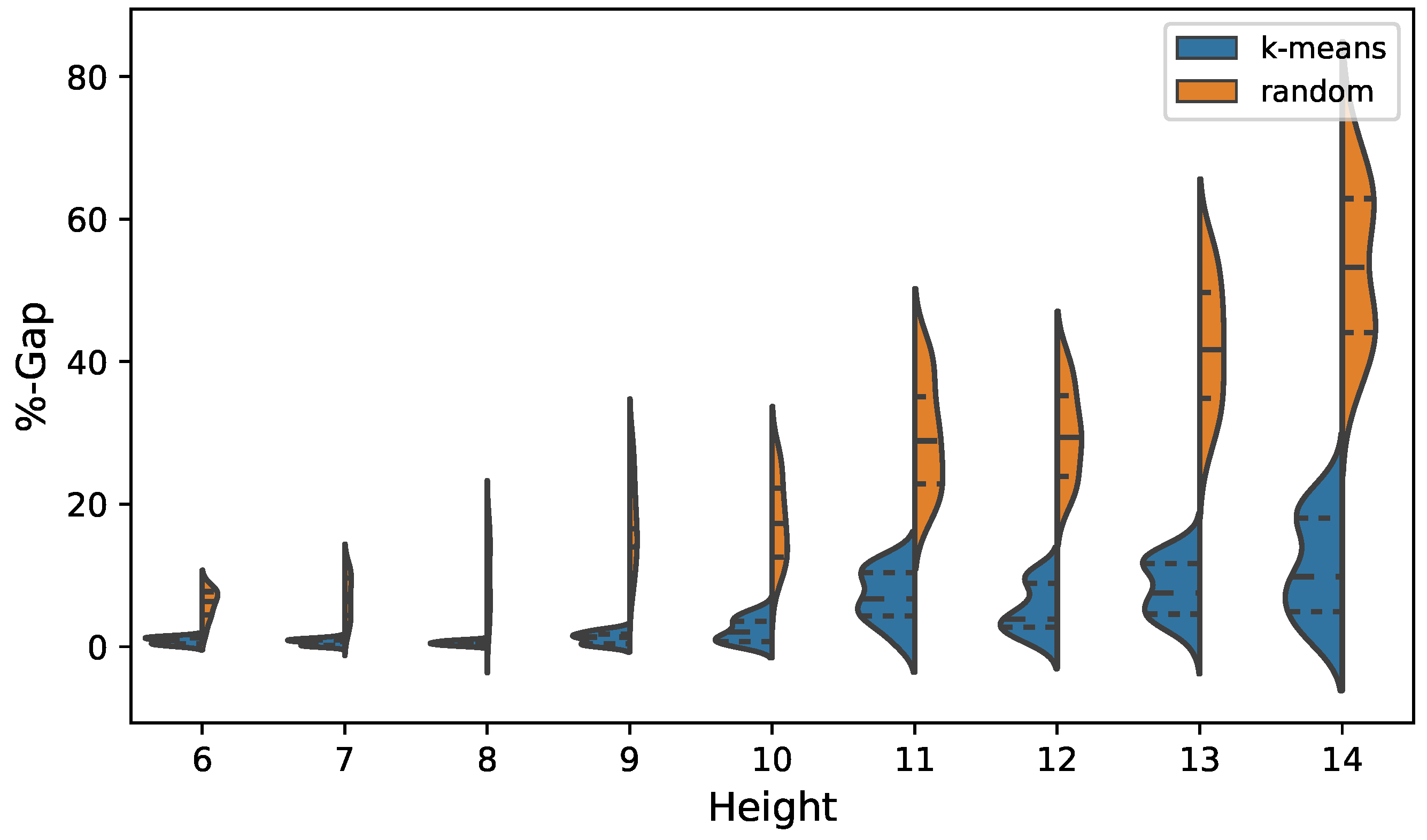
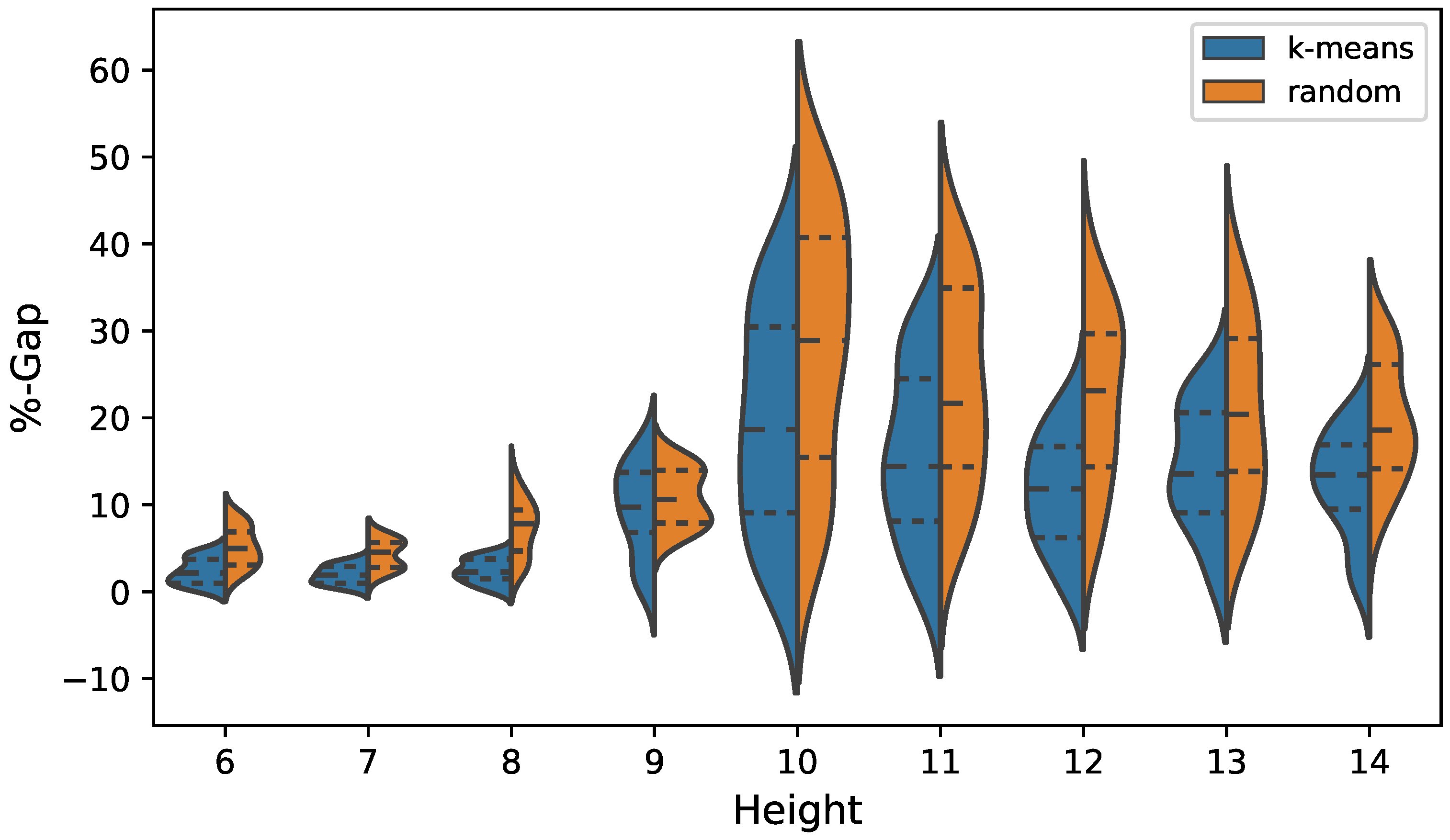
This experiment aims to quantify the contribution of the k-means operator in the process of optimizing the cost of the wall. To achieve this objective, a random operator was designed which replaces the k-means operator described in Section 4.2. This random operator behaves very similarly to that of k-means but instead of assigning transition probabilities per cluster, it assigns a fixed transition probability with a value of 0.5. In the experiment, wall height values between 6 and 14 m are considered. The k-means operator is compared with the random operator through the best value and the average obtained over 30 runs for each height. Later we will use the violin charts to compare both distributions of results and finally the Wilcoxon signed-rank test to validate that the difference is significant.
The results are shown in Table 5 and Figure 8 for cost optimization. In the case of emission optimization, the results are detailed in Figure 9 and in Table 6. In the case of cost optimization when analyzing the best value indicator, we observe that for all heights the k-means operator obtains better results compared to the random operator. In the case of a height of 6 and 7 m, this difference does not reach 2%. However, as the wall grows, the difference increases, reaching in the case of a height of 14 (m), 26%. The average indicator has similar behavior to that previously analyzed. The k-means operator has better performance in all cases. When applying the Wilcoxon test, it indicates that the difference is significant. When analyzing the distributions shown in Figure 8, we observe that the interquartile ranges obtained by the k-means operator are completely displaced to values close to zero with respect to the results obtained by the random operator. On the other hand, the dispersion of the distribution is greater in the solutions obtained by the random operator. In the case of optimization of CO2 emissions, when analyzing the best value indicator, we observe that the k-means operator obtains better results at all heights. However, the maximum difference from the random operator does not exceed 10%. The average indicator is again higher in the case of k-means, the Wilcoxon test indicating that the difference is significant. When analyzing the violin plots of the emissions shown in Figure 9, we see that the interquartile range obtains better quality results in the case of the k-means discretization. However, the result is not as remarkable as in the case of cost optimization.
Figure 10a,b show the convergence diagrams for cost optimization for the algorithm using k-means and random, respectively. The heights chosen were 6, 9, 12 and 14. From Figure 10a it is observed that heights 6 and 9 have a better convergence than in the case of 12 and 14. The same effect is observed for the case of the random operator, Figure 10b, although in the latter case it is not so notorious. When we make a comparison between the graphs, we observe for the random case the slope stabilizes much earlier than in the case of k-means, as a consequence of this the latter obtains better results.
5.3. Comparisons
To evaluate our algorithm in a different scenario than that of a random operator, in this Section we compare the results obtained by the algorithm that uses discretization by k-means, with the results published in [34,67]. In these works, the harmony search algorithm was used to optimize the buttress retaining wall. To evaluate the comparison, the best value will be analyzed for each of the different heights of the wall, in addition to comparing the distribution of the total solutions obtained for the different heights through violin plots. To determine that the difference is statistically significant, we will use the non-parametric Wilcoxon signed-rank test.
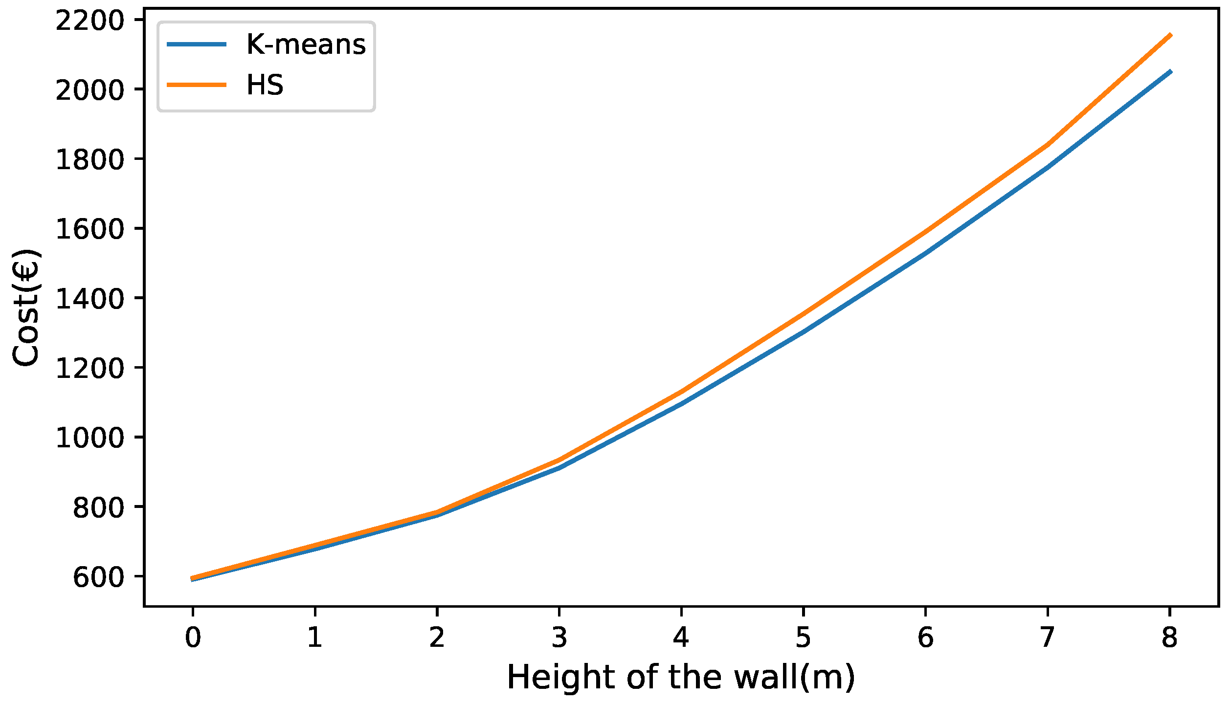
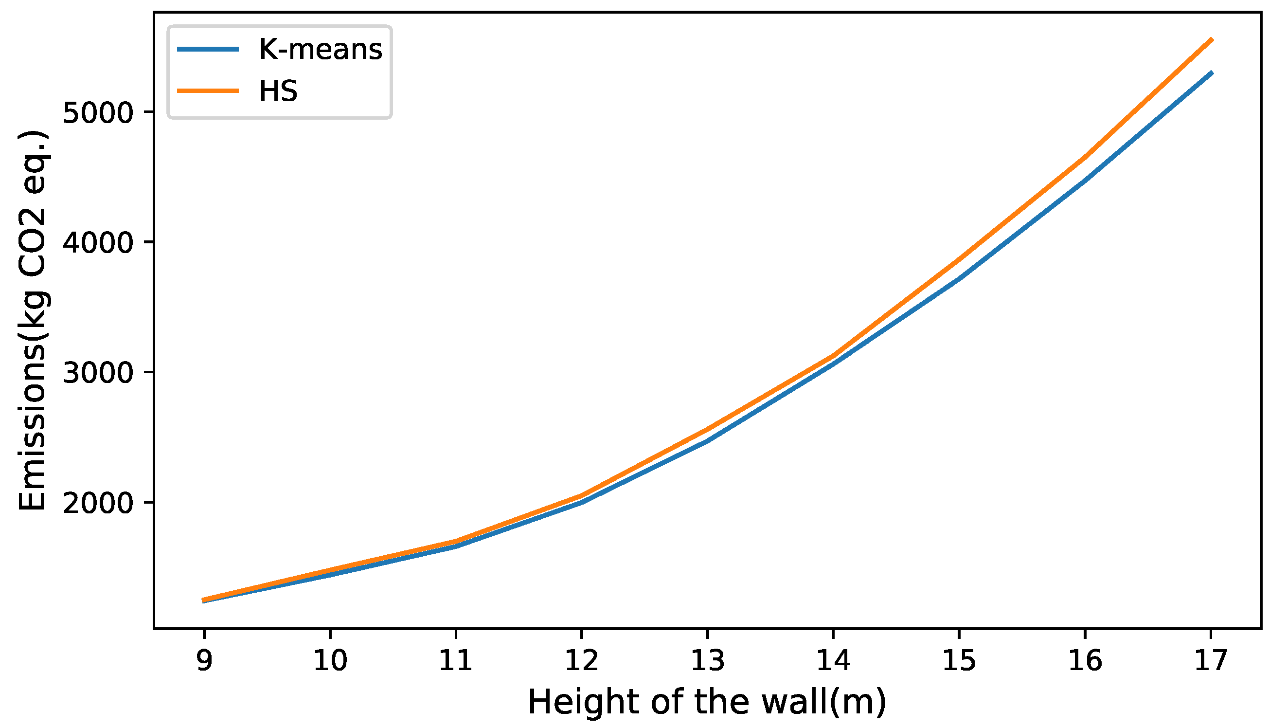
In Figure 11 and Figure 12, the best values obtained for the k-means and HS algorithms are compared. In the comparison, all the parameters were kept fixed except for the height, which like the previous experiments, varied from 6 to 14 m. When analyzing the heights of 6 to 8 m in Figure 11, it is observed that the cost of the solutions obtained by both algorithms is similar. As the wall grows in height, the curves have a greater separation, with the height of 14 (m) obtaining the greatest difference, this being 4.87% in favor of k-means. In the case of the comparison of the algorithms when optimizing the emissions of CO2, the curves behave similarly to that of the cost optimization case. For small values of wall height, very similar values are obtained. As the height of the wall increases, the quality of the k-means solutions improves compared to the HS. this is seen in Figure 12.
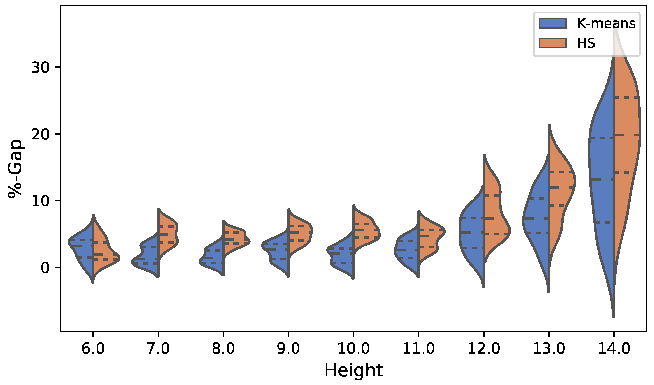
Figure 13 and Figure 14 show the comparison of the total solutions obtained by both algorithms. In the case of the cost optimization shown in Figure 13, we see that the interquartile range of the solutions obtained by k-means has better performance than those of HS. Up to height 12, the dispersion of the solutions is kept quite small in both algorithms. From height 12 onwards, this dispersion increases considerably in both k-means and HS. The case of the optimization of emissions presents a similar behavior, increasing its dispersion considerably from height 13. The above is observed in Figure 14.
6. Conclusions
In this article, a hybrid algorithm was proposed which uses the unsupervised k-means learning technique to construct discrete versions of optimization algorithms that work in continuous spaces. The optimization problem of a counterfort retaining wall was addressed, considering the cost and emission of CO2 as objective functions. The cuckoo search optimization algorithm was used to be discretized. Additionally, a random operator was constructed to determine the contribution of the k-mean operator in the optimization process. It was concluded that k-means produces better results than the random operator and in many cases this does it systematically, thus reducing the dispersion of the solutions. In addition, when we compare k-means with HS, we observe that as we increase the height, where the optimization problem becomes more difficult because it is more difficult to obtain stability of the wall with respect to overturning and sliding, k-means is more robust than HS reaching the height of 14 (m) at a difference of 4.76% in favor of k-means in optimizing emissions and 4.87% in minimizing costs. On the other hand, when we analyze the dispersion of the set of solutions, we see that k-means once again perform better than HS, especially for heights greater than 12 (m).
There are several possible directions for further extensions and improvements of the present work. The first line arises from observing the configuration parameters presented in Table 4. The configuration procedure can be simplified and improved by incorporating adaptive mechanisms that allow the parameters to be modified in accordance with the feedback obtained from the candidate solutions. A second line considers the incorporation of an intelligent agent that uses value gradient policies or action methods frequently used in reinforcement learning, in order to have information on the performance of the optimization algorithms with which we could modify the parameters dynamically. Finally, another possible line of research is to explore the population management of solutions dynamically. Through analyzing the history of exploration and exploitation of the search space, one can identify regions where it is necessary to increase the population and others where it is appropriate to decrease it.
Author Contributions
Conceptualization, V.Y., J.V.M. and J.G.; methodology, V.Y., J.V.M. and J.G.; software, J.V.M. and J.G.; validation, V.Y., J.V.M. and J.G.; formal analysis, J.G.; investigation, J.V.M. and J.G.; ; data curation, J.V.M.; writing—original draft preparation, J.G.; writing—review and editing, V.Y., J.V.M. and J.G.; funding acquisition, V.Y. and J.G. All authors have read and agreed to the published version of the manuscript.
Funding
The first author was supported by the Grant CONICYT/FONDECYT/INICIACION/11180056, the other two authors were supported by the Spanish Ministry of Economy and Competitiveness, along with FEDER funding (Project: BIA2017-85098-R)
Conflicts of Interest
The authors declare no conflict of interest.
References
- García, J.; Altimiras, F.; Peña, A.; Astorga, G.; Peredo, O. A binary cuckoo search big data algorithm applied to large-scale crew scheduling problems. Complexity 2018, 2018. [Google Scholar] [CrossRef]
- García, J.; Moraga, P.; Valenzuela, M.; Crawford, B.; Soto, R.; Pinto, H.; Peña, A.; Altimiras, F.; Astorga, G. A Db-Scan Binarization Algorithm Applied to Matrix Covering Problems. Comput. Intell. Neurosci. 2019, 2019. [Google Scholar] [CrossRef] [PubMed] [Green Version]
- Al-Madi, N.; Faris, H.; Mirjalili, S. Binary multi-verse optimization algorithm for global optimization and discrete problems. Int. J. Mach. Learn. Cybern. 2019, 10, 3445–3465. [Google Scholar] [CrossRef]
- Kim, M.; Chae, J. Monarch Butterfly Optimization for Facility Layout Design Based on a Single Loop Material Handling Path. Mathematics 2019, 7, 154. [Google Scholar] [CrossRef] [Green Version]
- García, J.; Crawford, B.; Soto, R.; Astorga, G. A clustering algorithm applied to the binarization of Swarm intelligence continuous metaheuristics. Swarm Evol. Comput. 2019, 44, 646–664. [Google Scholar] [CrossRef]
- García, J.; Lalla-Ruiz, E.; Voß, S.; Droguett, E.L. Enhancing a machine learning binarization framework by perturbation operators: Analysis on the multidimensional knapsack problem. Int. J. Mach. Learn. Cybern. 2020. [Google Scholar] [CrossRef]
- García, J.; Moraga, P.; Valenzuela, M.; Pinto, H. A db-Scan Hybrid Algorithm: An Application to the Multidimensional Knapsack Problem. Mathematics 2020, 8, 507. [Google Scholar] [CrossRef] [Green Version]
- Saeheaw, T.; Charoenchai, N. A comparative study among different parallel hybrid artificial intelligent approaches to solve the capacitated vehicle routing problem. Int. J. Bio-Inspir. Comput. 2018, 11, 171–191. [Google Scholar] [CrossRef]
- Crawford, B.; Soto, R.; Astorga, G.; García, J. Constructive metaheuristics for the set covering problem. In International Conference on Bioinspired Methods and Their Applications; Springer: Berlin, Germany, 2018; pp. 88–99. [Google Scholar]
- Valdez, F.; Castillo, O.; Jain, A.; Jana, D.K. Nature-inspired optimization algorithms for neuro-fuzzy models in real-world control and robotics applications. Comput. Intell. Neurosci. 2019, 2019, 9128451. [Google Scholar] [CrossRef]
- Penadés-Plà, V.; García-Segura, T.; Yepes, V. Robust Design Optimization for Low-Cost Concrete Box-Girder Bridge. Mathematics 2020, 8, 398. [Google Scholar] [CrossRef] [Green Version]
- García-Segura, T.; Yepes, V.; Frangopol, D.M.; Yang, D.Y. Lifetime reliability-based optimization of post-tensioned box-girder bridges. Eng. Struct. 2017, 145, 381–391. [Google Scholar] [CrossRef]
- Yepes, V.; Martí, J.V.; García, J. Black Hole Algorithm for Sustainable Design of Counterfort Retaining Walls. Sustainability 2020, 12, 2767. [Google Scholar] [CrossRef] [Green Version]
- Marti-Vargas, J.R.; Ferri, F.J.; Yepes, V. Prediction of the transfer length of prestressing strands with neural networks. Comput. Concr. 2013, 12, 187–209. [Google Scholar] [CrossRef]
- Fu, W.; Tan, J.; Zhang, X.; Chen, T.; Wang, K. Blind parameter identification of MAR model and mutation hybrid GWO-SCA optimized SVM for fault diagnosis of rotating machinery. Complexity 2019, 2019, 3264969. [Google Scholar] [CrossRef]
- Sierra, L.A.; Yepes, V.; García-Segura, T.; Pellicer, E. Bayesian network method for decision-making about the social sustainability of infrastructure projects. J. Clean. Prod. 2018, 176, 521–534. [Google Scholar] [CrossRef]
- Crawford, B.; Soto, R.; Astorga, G.; García, J.; Castro, C.; Paredes, F. Putting continuous metaheuristics to work in binary search spaces. Complexity 2017, 2017, 8404231. [Google Scholar] [CrossRef] [Green Version]
- Shi, Y. Particle swarm optimization: Developments, applications and resources. In Proceedings of the 2001 Congress on Evolutionary Computation, Seoul, Korea, 27–30 May 2001; Volume 1, pp. 81–86. [Google Scholar]
- Hatamlou, A. Black hole: A new heuristic optimization approach for data clustering. Inf. Sci. 2013, 222, 175–184. [Google Scholar] [CrossRef]
- Yang, X.S.; Deb, S. Cuckoo search via Lévy flights. In Proceedings of the 2009 World Congress on Nature & Biologically Inspired Computing (NaBIC), Coimbatore, India, 9–11 December 2009; pp. 210–214. [Google Scholar]
- Yang, X.S. A new metaheuristic bat-inspired algorithm. In Nature Inspired Cooperative Strategies for Optimization (NICSO 2010); Springer: Berlin, Germany, 2010; pp. 65–74. [Google Scholar]
- Yang, X.S. Firefly algorithms for multimodal optimization. In International Symposium on Stochastic Algorithms; Springer: Berlin, Germany, 2009; pp. 169–178. [Google Scholar]
- Pan, W.T. A new fruit fly optimization algorithm: Taking the financial distress model as an example. Knowl.-Based Syst. 2012, 26, 69–74. [Google Scholar] [CrossRef]
- Li, X.L.; Shao, Z.J.; Qian, J.X. An optimizing method based on autonomous animats: Fish-swarm algorithm. Syst. Eng. Theory Pract. 2002, 22, 32–38. [Google Scholar]
- Rashedi, E.; Nezamabadi-Pour, H.; Saryazdi, S. GSA: A gravitational search algorithm. Inf. Sci. 2009, 179, 2232–2248. [Google Scholar] [CrossRef]
- Calvet, L.; de Armas, J.; Masip, D.; Juan, A.A. Learnheuristics: Hybridizing metaheuristics with machine learning for optimization with dynamic inputs. Open Math. 2017, 15, 261–280. [Google Scholar] [CrossRef]
- Caserta, M.; Voß, S. Matheuristics: Hybridizing Metaheuristics and Mathematical Programming. In Metaheuristics: Intelligent Problem Solving; Springer: Berlin, Germany, 2009; pp. 1–38. [Google Scholar]
- Talbi, E.G. Combining metaheuristics with mathematical programming, constraint programming and machine learning. Ann. Oper. Res. 2016, 240, 171–215. [Google Scholar] [CrossRef]
- Juan, A.A.; Faulin, J.; Grasman, S.E.; Rabe, M.; Figueira, G. A review of simheuristics: Extending metaheuristics to deal with stochastic combinatorial optimization problems. Oper. Res. Perspect. 2015, 2, 62–72. [Google Scholar] [CrossRef] [Green Version]
- Chou, J.S.; Nguyen, T.K. Forward Forecast of Stock Price Using Sliding-Window Metaheuristic-Optimized Machine-Learning Regression. IEEE Trans. Ind. Inform. 2018, 14, 3132–3142. [Google Scholar] [CrossRef]
- Sayed, G.I.; Tharwat, A.; Hassanien, A.E. Chaotic dragonfly algorithm: An improved metaheuristic algorithm for feature selection. Appl. Intell. 2019, 49, 188–205. [Google Scholar] [CrossRef]
- De León, A.D.; Lalla-Ruiz, E.; Melián-Batista, B.; Moreno-Vega, J.M. A Machine Learning-based system for berth scheduling at bulk terminals. Expert Syst. Appl. 2017, 87, 170–182. [Google Scholar] [CrossRef]
- García, J.; Crawford, B.; Soto, R.; Castro, C.; Paredes, F. A k-means binarization framework applied to multidimensional knapsack problem. Appl. Intell. 2018, 48, 357–380. [Google Scholar] [CrossRef]
- Molina-Moreno, F.; Martí, J.V.; Yepes, V. Carbon embodied optimization for buttressed earth-retaining walls: Implications for low-carbon conceptual designs. J. Clean. Prod. 2017, 164, 872–884. [Google Scholar] [CrossRef]
- Voß, S. Meta-heuristics: The state of the art. In Workshop on Local Search for Planning and Scheduling; Springer: Berlin, Germany, 2000; pp. 1–23. [Google Scholar]
- Bishop, C.M. Pattern Recognition and Machine Learning; Springer: Berlin, Germany, 2006. [Google Scholar]
- Asta, S.; Özcan, E.; Curtois, T. A tensor based hyper-heuristic for nurse rostering. Knowl.-Based Syst. 2016, 98, 185–199. [Google Scholar] [CrossRef] [Green Version]
- Martin, S.; Ouelhadj, D.; Beullens, P.; Ozcan, E.; Juan, A.A.; Burke, E.K. A multi-agent based cooperative approach to scheduling and routing. Eur. J. Oper. Res. 2016, 254, 169–178. [Google Scholar] [CrossRef] [Green Version]
- García, J.; Crawford, B.; Soto, R.; Astorga, G. Astorga, G. A percentile transition ranking algorithm applied to binarization of continuous swarm intelligence metaheuristics. In International Conference on Soft Computing and Data Mining; Springer: Johor, Malaysia, 2018; pp. 3–13. [Google Scholar] [CrossRef]
- Vecek, N.; Mernik, M.; Filipic, B.; Xrepinsek, M. Parameter tuning with Chess Rating System (CRS-Tuning) for meta-heuristic algorithms. Inf. Sci. 2016, 372, 446–469. [Google Scholar] [CrossRef]
- Ries, J.; Beullens, P. A semi-automated design of instance-based fuzzy parameter tuning for metaheuristics based on decision tree induction. J. Oper. Res. Soc. 2015, 66, 782–793. [Google Scholar] [CrossRef] [Green Version]
- Li, Z.Q.; Zhang, H.L.; Zheng, J.H.; Dong, M.J.; Xie, Y.F.; Tian, Z.J. Heuristic evolutionary approach for weighted circles layout. In International Symposium on Information and Automation; Springer: Berlin, Germany, 2010; pp. 324–331. [Google Scholar]
- Yalcinoz, T.; Altun, H. Power economic dispatch using a hybrid genetic algorithm. IEEE Power Eng. Rev. 2001, 21, 59–60. [Google Scholar] [CrossRef]
- Kaur, H.; Virmani, J.; Thakur, S. A genetic algorithm-based metaheuristic approach to customize a computer-aided classification system for enhanced screen film mammograms. In U-Healthcare Monitoring Systems; Advances in Ubiquitous Sensing Applications for Healthcare; Dey, N., Ashour, A.S., Fong, S.J., Borra, S., Eds.; Academic Press: Cambridge, MA, USA, 2019; pp. 217–259. [Google Scholar] [CrossRef]
- Faris, H.; Hassonah, M.A.; Ala’M, A.Z.; Mirjalili, S.; Aljarah, I. A multi-verse optimizer approach for feature selection and optimizing SVM parameters based on a robust system architecture. Neural Comput. Appl. 2018, 30, 2355–2369. [Google Scholar] [CrossRef]
- Faris, H.; Aljarah, I.; Mirjalili, S. Improved monarch butterfly optimization for unconstrained global search and neural network training. Appl. Intell. 2018, 48, 445–464. [Google Scholar] [CrossRef]
- Chou, J.S.; Thedja, J.P.P. Metaheuristic optimization within machine learning-based classification system for early warnings related to geotechnical problems. Autom. Constr. 2016, 68, 65–80. [Google Scholar] [CrossRef]
- Pham, A.D.; Hoang, N.D.; Nguyen, Q.T. Predicting compressive strength of high-performance concrete using metaheuristic-optimized least squares support vector regression. J. Comput. Civ. Eng. 2015, 30, 06015002. [Google Scholar] [CrossRef]
- Göçken, M.; Özçalıcı, M.; Boru, A.; Dosdoğru, A.T. Integrating metaheuristics and artificial neural networks for improved stock price prediction. Expert Syst. Appl. 2016, 44, 320–331. [Google Scholar] [CrossRef]
- Chou, J.S.; Pham, A.D. Nature-inspired metaheuristic optimization in least squares support vector regression for obtaining bridge scour information. Inf. Sci. 2017, 399, 64–80. [Google Scholar] [CrossRef]
- Kuo, R.; Lin, T.; Zulvia, F.; Tsai, C. A hybrid metaheuristic and kernel intuitionistic fuzzy c-means algorithm for cluster analysis. Appl. Soft Comput. 2018, 67, 299–308. [Google Scholar] [CrossRef]
- Mann, P.S.; Singh, S. Energy efficient clustering protocol based on improved metaheuristic in wireless sensor networks. J. Netw. Comput. Appl. 2017, 83, 40–52. [Google Scholar] [CrossRef]
- De Alvarenga Rosa, R.; Machado, A.M.; Ribeiro, G.M.; Mauri, G.R. A mathematical model and a Clustering Search metaheuristic for planning the helicopter transportation of employees to the production platforms of oil and gas. Comput. Ind. Eng. 2016, 101, 303–312. [Google Scholar] [CrossRef]
- Faris, H.; Mirjalili, S.; Aljarah, I. Automatic selection of hidden neurons and weights in neural networks using grey wolf optimizer based on a hybrid encoding scheme. Int. J. Mach. Learn. Cybern. 2019, 10, 2901–2920. [Google Scholar] [CrossRef]
- De Rosa, G.H.; Papa, J.P.; Yang, X.S. Handling dropout probability estimation in convolution neural networks using meta-heuristics. Soft Comput. 2018, 22, 6147–6156. [Google Scholar] [CrossRef] [Green Version]
- Tuba, M.; Alihodzic, A.; Bacanin, N. Cuckoo search and bat algorithm applied to training feed-forward neural networks. In Recent Advances in Swarm Intelligence and Evolutionary Computation; Springer: Berlin, Germany, 2015; pp. 139–162. [Google Scholar]
- Rere, L.; Fanany, M.I.; Arymurthy, A.M. Metaheuristic algorithms for convolution neural network. Comput. Intell. Neurosci. 2016, 2016, 1537325. [Google Scholar] [CrossRef] [PubMed] [Green Version]
- Rashid, T.A.; Hassan, M.K.; Mohammadi, M.; Fraser, K. Improvement of variant adaptable LSTM trained with metaheuristic algorithms for healthcare analysis. In Advanced Classification Techniques for Healthcare Analysis; IGI Global: Hershey, PA, USA, 2019; pp. 111–131. [Google Scholar]
- Jothi, R.; Mohanty, S.K.; Ojha, A. DK-means: A deterministic k-means clustering algorithm for gene expression analysis. Pattern Anal. Appl. 2019, 22, 649–667. [Google Scholar] [CrossRef]
- García, J.; Pope, C.; Altimiras, F. A Distributed-Means Segmentation Algorithm Applied to Lobesia botrana Recognition. Complexity 2017, 2017, 5137317. [Google Scholar] [CrossRef] [Green Version]
- Arunkumar, N.; Mohammed, M.A.; Ghani, M.K.A.; Ibrahim, D.A.; Abdulhay, E.; Ramirez-Gonzalez, G.; de Albuquerque, V.H.C. K-means clustering and neural network for object detecting and identifying abnormality of brain tumor. Soft Comput. 2019, 23, 9083–9096. [Google Scholar] [CrossRef]
- Abdel-Basset, M.; Wang, G.G.; Sangaiah, A.K.; Rushdy, E. Krill herd algorithm based on cuckoo search for solving engineering optimization problems. Multimed. Tools Appl. 2019, 78, 3861–3884. [Google Scholar] [CrossRef]
- Chi, R.; Su, Y.X.; Zhang, D.H.; Chi, X.X.; Zhang, H.J. A hybridization of cuckoo search and particle swarm optimization for solving optimization problems. Neural Comput. Appl. 2019, 31, 653–670. [Google Scholar] [CrossRef]
- Li, J.; Xiao, D.D.; Lei, H.; Zhang, T.; Tian, T. Using Cuckoo Search Algorithm with Q-Learning and Genetic Operation to Solve the Problem of Logistics Distribution Center Location. Mathematics 2020, 8, 149. [Google Scholar] [CrossRef] [Green Version]
- Pan, J.S.; Song, P.C.; Chu, S.C.; Peng, Y.J. Improved Compact Cuckoo Search Algorithm Applied to Location of Drone Logistics Hub. Mathematics 2020, 8, 333. [Google Scholar] [CrossRef]
- Yepes, V.; Alcala, J.; Perea, C.; González-Vidosa, F. A parametric study of optimum earth-retaining walls by simulated annealing. Eng. Struct. 2008, 30, 821–830. [Google Scholar] [CrossRef]
- Molina-Moreno, F.; García-Segura, T.; Martí, J.V.; Yepes, V. Optimization of buttressed earth-retaining walls using hybrid harmony search algorithms. Eng. Struct. 2017, 134, 205–216. [Google Scholar] [CrossRef]
- Ministerio de Fomento. EHE: Code of Structural Concrete; Ministerio de Fomento: Madrid, Spain, 2008. [Google Scholar]
- Ministerio de Fomento. CTE. DB-SE. Structural Safety: Foundations; Ministerio de Fomento: Madrid, Spain, 2008. (In Spanish)
- Huntington, W.C. Earth Pressures and Retaining Walls; Literary Licensing, LLC: Whitefish, MT, USA, 1957. [Google Scholar]
- Calavera, J. Muros de Contención y Muros de Sótano; INTEMAC: Madrid, Spain, 2001. (In Spanish) [Google Scholar]
- CEB-FIB. Model Code. Design Code; Thomas Telford Services Ltd.: London, UK, 2008. [Google Scholar]
- Hays, W.L.; Winkler, R.L. Statistics: Probability, Inference, and Decision; Holt, Rinehart, and Winston: New York, NY, USA, 1971. [Google Scholar]
- Wilcoxon, F. Individual comparisons by ranking methods. In Breakthroughs in Statistics; Springer: Berlin, Germany, 1992; pp. 196–202. [Google Scholar]
Figure 1.
General scheme: Combining Machine Learning and Metaheuristics.

Figure 2.
Reinforcement variables for the design of earth-retaining walls. Source: [67].
Figure 2.
Reinforcement variables for the design of earth-retaining walls. Source: [67].

Figure 3.
Earth-retaining buttressed wall. Floor cross-section. Source: [67].
Figure 3.
Earth-retaining buttressed wall. Floor cross-section. Source: [67].

Figure 4.
Problem design parameters. Source: [67].
Figure 4.
Problem design parameters. Source: [67].

Figure 5.
Solution initiation procedure.

Figure 6.
The discrete k-means algorithm flow chart.

Figure 7.
Flow chart of parameter setting.

Figure 8.
Cost violin plots, comparison between k-means and random operators.

Figure 9.
Emission Violin plots, comparison between k-means and random operators.

Figure 10.
K-means and Random convergence chart for cost optimization.

Figure 11.
Comparison between the best solutions obtained by the k-means and HS algorithms in cost optimization.
Figure 11.
Comparison between the best solutions obtained by the k-means and HS algorithms in cost optimization.

Figure 12.
Comparison between the best solutions obtained by the k-means and HS algorithms in emission optimization.
Figure 12.
Comparison between the best solutions obtained by the k-means and HS algorithms in emission optimization.

Figure 13.
Violin plot comparison between k-means and HS results for cost in euros.

Figure 14.
Violin plot comparison between k-means and HS results for CO2 emissions.


Table 1.
Unit breakdown of emissions and cost.
| Unit | Emissions (CO2-eq) | Cost (€) |
|---|---|---|
| kg of steel B400 | 3.02 | 0.56 |
| kg of steel B500 | 2.82 | 0.58 |
| m3 of concrete HA-25 in stem | 224.34 | 56.66 |
| m3 of concrete HA-30 in stem | 224.94 | 60.80 |
| m3 of concrete HA-35 in stem | 265.28 | 65.32 |
| m3 of concrete HA-40 in stem | 265.28 | 70.41 |
| m3 of concrete HA-45 in stem | 265.91 | 75.22 |
| m3 of concrete HA-50 in stem | 265.95 | 80.03 |
| m2 stem formwork | 1.92 | 21.61 |
| m3 of backfill | 28.79 | 5.56 |
| m3 of concrete HA-25 in foundation | 224.34 | 50.65 |
| m3 of concrete HA-30 in foundation | 224.94 | 54.79 |
| m3 of concrete HA-35 in foundation | 265.28 | 59.31 |
| m3 of concrete HA-40 in foundation | 265.28 | 64.40 |
| m3 of concrete HA-45 in foundation | 265.91 | 69.21 |
| m3 of concrete HA-50 in foundation | 265.95 | 74.02 |
Table 2.
Design variables.
| Variables | Lower Bound | Increment | Upper Bound | N of Values |
|---|---|---|---|---|
| c | H/20 | 5 cm | H/5 | f(H) 1 |
| b | 25 cm | 2.5 cm | 122.5 | 40 |
| p | 20 cm | 10 cm | 610 | 60 |
| t | 20 cm | 15 cm | 905 | 60 |
| 25 cm | 2.5 cm | 122.5 | 40 | |
| d | H/5 cm | 5 cm | 2H/3 | f(H) 1 |
| 25, 20, 25, 40, 45, 50 | 7 | |||
| 400, 500 | 2 | |||
| to | 6, 8, 10, 12, 16, 20, 25, 32 | 8 | ||
| 1 steel rebar | 2 rebars | 12 rebars | 6 | |
| to | 6, 8, 10, 12, 16, 20, 25, 32 | 8 | ||
| 1 steel rebar | 4 rebars | 10 rebars | 7 |
(1) Number of values depends on the height.
Table 3.
Problem design parameters values.
| Parameter Considered | Value |
|---|---|
| Bearing capacity | 0.3 MPa |
| Fill slope | 0 |
| Foundation depth, H2 | 2 m |
| Uniform load on top of the fill, | 10 kN/m2 |
| Wall-fill friction angle, | 0° |
| Base-friction coefficient, | tg 30° |
| Safety coefficient against sliding, | 1.5 |
| Safety coefficient against overturning, | 1.8 |
| EHE safety coefficient for loading | Normal |
| ULS safety coefficient of concrete | 1.5 |
| ULS safety coefficient of steel | 1.15 |
| EHE ambient exposure | IIa |
Table 4.
Parameter setting for the Cuckoo search algorithm.
| Parameters | Description | Value | Range |
|---|---|---|---|
| N | Number of Nest | 5 | [5, 10, 15] |
| k | Number of transition groups K-means Operator | 5 | [4, 5, 6] |
| Step Length | 0.01 | 0.01 | |
| Lévy distribution parameter | 1.5 | 1.5 | |
| Iteration Number | Maximum iterations | 800 | [800] |
Table 5.
Comparison between random and k-means operators in cost optimization.
| Height (m) | Best Value | Avg | Best Value | Avg | Best Value | Avg Random |
|---|---|---|---|---|---|---|
| k-Means | k-Means | Random | Random | HS | HS | |
| 6 | 591 | 595.5 | 600 | 621.3 | 595 | 600.15 |
| 7 | 678 | 682.8 | 687 | 721.4 | 689 | 694.98 |
| 8 | 775 | 778.9 | 785 | 851.7 | 784 | 788.38 |
| 9 | 911 | 922.3 | 981 | 1094.3 | 934 | 941.29 |
| 10 | 1095 | 1127.0 | 1184 | 1296.7 | 1130 | 1143.64 |
| 11 | 1302 | 1384.5 | 1545 | 1704.5 | 1354 | 1381.50 |
| 12 | 1528 | 1608.9 | 1839 | 1994.3 | 1590 | 1707.24 |
| 13 | 1775 | 1905.3 | 2241 | 2510.8 | 1840 | 2067.37 |
| 14 | 2049 | 2301.6 | 2775 | 3267.1 | 2154 | 2348.71 |
| Wilcoxon p-value | 1.6 × 10⁻⁵ | 1.31 × 10⁻³ |
Table 6.
Comparison between random and k-means operators in emission optimization.
| Height (m) | Best Value | Avg | Best Value | Avg | Best Value | Avg Random |
|---|---|---|---|---|---|---|
| k-Means | k-Means | Random | Random | HS | HS | |
| 6 | 1242 | 1251.2 | 1274 | 1304.3 | 1250 | 1289.14 |
| 7 | 1440 | 1458.5 | 1467 | 1501.3 | 1478 | 1511.53 |
| 8 | 1659 | 1683.2 | 1696 | 1788.6 | 1699 | 1731.54 |
| 9 | 1997 | 2111.1 | 2180 | 2214.6 | 2050 | 2097.45 |
| 10 | 2470 | 2572.1 | 2975 | 3132.7 | 2560 | 2617.81 |
| 11 | 3061 | 3206.6 | 3540 | 3801.7 | 3124 | 3201.45 |
| 12 | 3715 | 3921.5 | 4168 | 4555.7 | 3865 | 4046.95 |
| 13 | 4470 | 4676.4 | 5039 | 5484.5 | 4650 | 4955.95 |
| 14 | 5294 | 5621.2 | 5877 | 6319.1 | 5550 | 6241.00 |
| Wilcoxon p-value | 1.2 × 10⁻⁷ | 2.51 × 10⁻⁴ |
© 2020 by the authors. Licensee MDPI, Basel, Switzerland. This article is an open access article distributed under the terms and conditions of the Creative Commons Attribution (CC BY) license (http://creativecommons.org/licenses/by/4.0/).
Share and Cite
MDPI and ACS Style
García, J.; Yepes, V.; Martí, J.V. A Hybrid k-Means Cuckoo Search Algorithm Applied to the Counterfort Retaining Walls Problem. Mathematics 2020, 8, 555. https://doi.org/10.3390/math8040555
AMA Style
García J, Yepes V, Martí JV. A Hybrid k-Means Cuckoo Search Algorithm Applied to the Counterfort Retaining Walls Problem. Mathematics. 2020; 8(4):555. https://doi.org/10.3390/math8040555
Chicago/Turabian StyleGarcía, José, Victor Yepes, and José V. Martí. 2020. "A Hybrid k-Means Cuckoo Search Algorithm Applied to the Counterfort Retaining Walls Problem" Mathematics 8, no. 4: 555. https://doi.org/10.3390/math8040555
Note that from the first issue of 2016, this journal uses article numbers instead of page numbers. See further details here.