Reducing the Cost of Electricity by Optimizing Real-Time Consumer Planning Using a New Genetic Algorithm-Based Strategy


.jpg)
1
Faculty of Electronics, Communications and Computers, University of Pitesti, Targul din Vale 1, 110040 Pitesti, Romania
2
Faculty of Mechanics and Technology, University of Pitesti, Targul din Vale 1, 110040 Pitesti, Romania
*
Authors to whom correspondence should be addressed.
Mathematics 2020, 8(7), 1144; https://doi.org/10.3390/math8071144
Submission received: 3 June 2020
/
Revised: 8 July 2020
/
Accepted: 10 July 2020
/
Published: 13 July 2020
(This article belongs to the Special Issue Advanced Modeling and Research in Hybrid Microgrid Control and Optimization)
Abstract
:To ensure the use of energy produced from renewable energy sources, this paper presents a method for consumer planning in the consumer–producer–distributor structure. The proposed planning method is based on the genetic algorithm approach, which solves a cost minimization problem by considering several input parameters. These input parameters are: the consumption for each unit, the time interval in which the unit operates, the maximum value of the electricity produced from renewable sources, and the distribution of energy production per unit of time. A consumer can use the equipment without any planning, in which case he will consume energy supplied by a distributor or energy produced from renewable sources, if it is available at the time he operates the equipment. A consumer who plans his operating interval can use more energy from renewable sources, because the planning is done in the time interval in which the energy produced from renewable sources is available. The effect is that the total cost of energy to the consumer without any planning will be higher than the cost of energy to the consumer with planning, because the energy produced from renewable sources is cheaper than that provided from conventional sources. To be validated, the proposed approach was run on a simulator, and then tested in two real-world case studies targeting domestic and industrial consumers. In both situations, the solution proposed led to a reduction in the total cost of electricity of up to 25%.
1. Introduction
Through the range of energy producers, from small (photovoltaic panels at the level of households) and medium (fields of photovoltaic panels, wind power plants) producers, to large traditional electricity producers (hydroelectric power stations, thermal power plants, nuclear power plants), the need to expand power networks has emerged. The tendency is to implement on-demand electricity production and distribution techniques according to consumer’s needs. On the one hand, these consumers are increasing in number and have steadily increasing needs. On the other hand, producers of electricity from renewable sources are less likely to adapt their production capacity according to the consumers’ requirements.
The use of smart grids and the concepts derived from it, such as dynamic prices and demand management, have had a significant impact in many areas.
An alternative to production management and the distribution of electricity on demand is to apply dynamic tariff plans. Such plans motivate consumers to save electricity during some periods by re-scheduling household activities (chores) to other time periods. Thus, the distribution of total electricity consumption becomes uniform over time by eliminating the consumption peaks in some short time intervals. Dynamic tariff schemes can be changed according to area and consumption time interval. Several studies [1] show that a dynamic price of electricity reduces electricity costs at the level of consumers by as much as 10%. Dynamic pricing favors the consumption of electricity during periods when energy producers from renewable sources can supply this energy.
The main problem related to the production and distribution of electricity on demand and the dynamic pricing of electricity is the real-time monitoring of consumers—it is necessary to determine the energy consumption for short periods of time in order to apply differential tariffing. The existing meters in the electricity distributors’ infrastructure have two limitations: they only have a local, short-range communication interface to an operator, and they do not transmit the data acquired in real-time. A third limitation is related to the fixed location of the meter, i.e., at the level of a consumer or at the level of a grid node. Thus, it can either provide a small amount of data regarding the status of a single consumer, which cannot be used in a statistical analysis without violating the consumer’s right to privacy, or too large amounts of data regarding the status of an entire grid. In the second case, the status of different branches, in terms of new consumers attaching to a node, modifications of the electricity grid, appearance of new grid nodes, etc., cannot be seen.
The real-time monitoring of electricity consumption (current and voltage) at different points of the electricity distribution grid is therefore an essential element in dynamic pricing. It is important to use non-invasive solutions that monitor electricity consumption, which can be easily placed in the existing electricity distribution infrastructure. The main problem when measuring energy consumption is the measurement of current consumption. This involves mounting the ammeter in series on the power cable. There are several technologies that allow for electricity measurement without the need for infrastructure intervention.
The current consumption sensor is the main component of a monitoring system for consumer planning and dynamic pricing. For an autonomous solution, the main requirement is that the sensor allows for energy harvesting.
Our paper proposes a consumer planning solution, using a genetic algorithm (GA), to reduce the consumer electricity cost by using as much electricity as possible from renewable sources by local micro-producers. The novel elements presented in this paper compared to previous publications and research projects are as follows:
- -
- The use of a genetic algorithm for the re-planning of consumers to reduce the electricity cost using the energy of local producers through renewable means. The use of a genetic algorithm for consumer planning and the way in which the coding solution was realized (i.e., obtaining the chromosome) are the original components of the paper.
- -
- The implementation of a simulator that allows the generation of numerous consumer–producer configurations (i.e., hundreds), and the study of the impact of the consumer planning algorithm.
- -
- A complete platform implemented for real-time consumption monitoring, analysis, and intelligent planning, using the genetic algorithm, and consumer communication/information. Unlike other works in the field, this paper presents a complete solution that allows for the implementation of a consumer planning algorithm that consists of sensor cells for the acquisition of current consumption with self-harvesting, data collectors, a server for analysis and planning, and a client application for informing consumers. The system, developed as part of a research project, was used in two case studies that highlight the efficiency of the consumer planning algorithm.
There are several solutions proposed for consumer planning. They have different approaches to re-planning consumers in order to reduce the total cost of electricity. In contrast, the solution proposed in this paper addresses the issue of consumer planning from multiple perspectives: the ability to produce electricity through renewable means at different times of the day, for certain regions and using different energy sources; the cost of electricity produced from renewable sources; the cost of electricity produced by traditional methods; and the characteristics of some consumers to be able to be reprogrammed at longer or shorter time intervals. All of these elements represent criteria that must be taken into account when determining the optimal planning scheme of consumption units (equipment) during a day, to finally obtain the minimum cost of electricity. The genetic algorithm is an algorithm specialized in solving multi-criteria optimization problems: this is the reason why this type of algorithm was used here.
The objectives of this study are as follows:
- proposing a new strategy to reduce the electricity cost in a nano- or micro-grid through optimal consumer planning;
- implementing the proposed strategy in a simulator (using Python libraries, such as Numpy and Matplotlib);
- validation of simulation results in two experiments, using an innovative genetic algorithm proposed and analyzed in this paper;
- highlighting the advantages for all participants (micro-producers, regular consumers, or prosumers) based on case studies where this strategy was implemented.
The next section will present strategies from the specialized literature that are designed to reduce the electricity cost in a smart grid through optimal consumer planning.
Compared to the previous publications and research projects presented below, the novelty of this paper is highlighted as follows: (1) a new real-time optimization strategy based on an objective function to minimize the total cost by planning consumers to use available electricity produced from renewable sources is proposed; (2) a new chromosome coding solution is proposed and used by the genetic algorithm applied to reduce the electricity cost.
The validation of the reduction of the energy cost for a consumer who applies this new strategy was conducted both in simulation and in experiment. For this, a specific simulator and a complete experimental platform were implemented to evaluate the performance of the proposed strategy, based on hundreds of consumer–producer configurations and case studies emulating the functioning of a smart nano-grid. The experiment was developed as part of a research project (using sensor cells for the acquisition of current consumption with self-harvesting, data collectors, a server for analysis and planning, a client application for informing consumers, etc.), in order to emulate the functioning of a smart nano-grid as closely as possible to reality. For both implementations, the genetic algorithm optimizes the cost function for the consumer taking into account the requirements and constraints imposed (for example, times when devices have to be used, electricity available from renewable sources), which are variable over time. The only difference for the performed experiments is that the input data (such as the possible operating interval and the actual operating interval for consumers, and the cost of energy produced, the available production capacity, and the daily variation in production capacity for producers) are acquired from installed sensors at consumers and producers, rather than simulated data. Thus, the originality of the paper is related to the development and implementation of the consumer planning algorithm on the central station server, as well as to the implementation plan to easily apply the platform in various experimental case studies.
The remainder of this paper is structured as follows: Section 2 presents a literature review. The subsequent section presents the model and coding schema used for the genetic algorithm, and is divided into four subsections: Section 3.1 The Consumer–Producer–Distributor Mode, Section 3.2 Genetic Algorithm, Section 3.3 Simulation Platform and Data Collection, and Section 3.4 Methods. Section 4.1 presents the simulation and the results obtained from the simulation, and Section 4.2 presents the system implementation and its operation in two real case studies. The paper concludes with Section 5 Conclusions and Future Trends.
2. Literature Review
In reference [2], a comprehensive study of the use of the smart grid in communication infrastructure to reduce energy consumption is offered. The study begins by addressing the concept of the smart grid, and continues with the presentation of smart grid techniques for increasing energy efficiency in communications, and minimizing energy costs and emissions of data centers and cloud infrastructures. This is the also the purpose pursued in our work. The objective of the current study is to carry out a re-planning of consumers in order to reduce the cost of electricity. This is possible using the proposed real-time monitoring platform, as presented in this paper. Alahakoon et al. [3] present a comprehensive study of smart grids and their use, technologies used in the metering process, and solutions to satisfy the interests of stakeholders. Moreover, the paper highlights challenges and opportunities that arise using big data and the cloud in smart grids. Problems relating to data privacy in smart grids (SGs) and advanced measurement infrastructure (AMI) are treated in reference [4]. The use of SGs and AMI allows the implementation of consumer planning solutions through the possibility of real-time monitoring on different nodes of the distribution network. However, at present, the monitoring infrastructure is not always available for real-time monitoring. This is the reason why, in our paper, a flexible monitoring solution is proposed, which allows real-time monitoring for the application of dynamic tariffs, and to favor the consumption of electricity from renewable sources. After data acquisition, it is necessary to analyze them, and to develop consumption planning. Deng et al. [5] refer to energy consumption planning using a game model. As a result, consumption peaks are reduced. The issue of consumer planning following the reprogramming of processes with the implementation of a simulator is addressed by Kliazovich et al. [6]. Tang et al. [7] address the reprogramming of tasks (at a certain manufacturing process) in order to reduce energy consumption. Starting from the characteristics of the production process, the consumption pattern is determined by a model developed in reference [8]. A genetic algorithm is then used to determine which of the elaborated schemes is optimal. The key element in the consumer planning solution proposed in the current paper is also a genetic algorithm. Unlike the mentioned works, consumers’ planning is realized to reduce the total cost of electricity, with a flexible configuration scheme that applies to both domestic and industrial consumers. This is done by the coding schema performed on the genetic algorithm.
Previous studies have dealt with the problem of consumer planning and have proposed different algorithms for solving it. Cionca et al. [9] refer to the planning of the energy produced and consumed to accumulate surpluses and to reduce losses (which occur when there is a surplus of produced energy). Derakhshan et al. [10] present algorithms for energy consumption: Teaching and Learning-based Optimization (TLBO) and Shuffled Frog Leaping (SFL). These are applied to a case study for a real environment. As with our approach, in the above-mentioned work, the total energy cost is reduced by reducing the costs for certain periods using the electricity produced from unconventional sources. Ghasemi et al. [11] propose a new algorithm for forecasting the electricity price and its demand, which uses data preprocessing techniques, forecasting, and adjustment algorithms. The three components of the forecasting algorithm are described, including an artificial intelligence (AI) component of the artificial bee colony (ABC) type used in the learning process. This generates coefficients for the other modules. The proposed hybrid forecast algorithm is evaluated on several real markets, illustrating its high accuracy in the forecast of the price and demand of electricity. Moreover, the impact of its use on demand management techniques is investigated, emphasizing the improvements made.
Ma et al. [12] present a new concept of a residential consumption planning framework based on cost efficiency. Cost efficiency means the ratio between the total benefit and the total payment of electricity over a certain period. In this work, a consumption planning algorithm based on daily costs is developed using a fractional programming approach. The proposed planning algorithm can reflect and affect consumer behavior, and ultimately generate an optimal cost-effective energy consumption profile. Similarly, in the current paper, the planning of consumption units takes place, but the cost is related to the method of obtaining the electricity.
The aforementioned paper presents a simulation that confirms that the proposed planning algorithm significantly improves cost efficiency for consumers compared to conventional planning solutions. In a similar way, a simulator is also created for validating the efficiency of the proposed consumer planning algorithm. Moreover, the algorithm is implemented using a real-time monitoring platform and results for two real-world case studies are presented.
During the implementation of the platform, there are several challenges related, in particular, to connecting the current sensors to the electricity transmission lines and their power supply. On this topic, several studies have been conducted of the construction of the monitoring platform and the implementation of the algorithm. Along with solutions with neural networks and GAs, other algorithms have been used to reduce consumption and plan hybrid energy sources. Thus, the paper [13] presents an algorithm-based chaotic search and harmony search, which is used to plan the storage of energy produced from five renewable sources (photovoltaic and wind). A system composed of a chemical cell based on hydrogen and a battery is used for energy storage and the objective is to extend the life of the storage cells and reduce the cost by optimally planning the storage sequence (charges/discharges). In our case, a GA is used to plan the operating time interval in order to use as much energy as possible from renewable sources. A novel particle swarm optimization algorithm based on the Hill function is presented in paper [14] for reducing energy consumption in an industrial process by dynamically planning its component tasks. We propose a similar task in our paper, but we address a much wider category of consumers. Our goal is not to reduce energy consumption but to reduce the cost of energy by using renewable sources. An energy management system produced from three different sources (renewable with photovoltaic panels, batteries, and generator with a diesel engine) based on a modified gravitational search algorithm is presented in [15]. Here, a solution is provided by which to choose one of the three sources to meet the needs of the consumer while reducing fuel consumption as much as possible, and extending battery life. The solution we propose is aimed at consumer-level programming to reduce the cost of energy using energy from different sources. Our approach is somewhat more general—it aims to provide solutions for a wide range of consumers and producers of energy from renewable sources. The solution we propose is based on GA but can be extended with other algorithms, such as the whale optimization algorithm (WOA).
The use of genetic algorithms for consumer planning to reduce the cost of electricity is a subject that has also been addressed in very recent works and research (2019). Xu et al. [16] used a genetic algorithm to plan the operation of an irrigation system so that it is used when the cost of energy is lower; thus, the goal is to reduce the cost of electricity. The solution proposed in the current paper is also the application of an optimization problem to reduce the cost of electricity. However, our approach involves, more generally, the planning of different consumers, in order to reduce the cost of electricity. Another GA-based approach, applied in an industrial environment, is presented in reference [17]. Here, it was used in the planning of an automatic guided vehicle (AGV) inside a factory, to make electricity consumption more efficient. Chang et al. [18] illustrate a solution for planning the operation of heating, ventilation, and air conditioning (HVAC) equipment through a neuro-genetic hybrid solution, to reduce annual energy consumption. The work addresses an optimization problem that aims to reduce cost and increase satisfaction among the tenants in the building connected to the air conditioning system. Farhadiana [19] presents a solution for planning how to allocate virtual machines on physical equipment considering the operation and the resources used by each one. The objective is to reduce energy consumption—allocation planning is undertaken through a genetic algorithm solution. Our approach brings, as a novelty element, the coding scheme proposed in the genetic algorithm that allows the planning of different consumers. The objective function is to minimize the total cost of planning consumers, to use electricity produced from renewable sources when it is available.
The involvement of consumers in the process of planning the operation of electrical appliances to reduce the cost of electricity is a modern trend, as shown in Gram-Hanssen et al. [20]. The authors state that such policies have a direct impact on the environment by reducing carbon emissions and the use of renewable energy sources. It is shown that, for a sample of about 2000 people surveyed, 75% stated that they are interested in re-planning consumers to use more renewable energy. This idea is taken up in the present paper. Moreover, its authors propose a solution to help the consumer plan in the most efficient way. Along with the desire to protect the environment, the consumer must also be materially motivated. For this reason, a consumer profile must be determined and then associated with a tariff scheme. Some consumer profiles use more energy from renewable sources and lead to a lower total cost. Determining a consumer’s profile is not easy. It depends on the type of consumption units (equipment) but also on its needs. That is why different algorithms are used to identify the profile. In reference [21], the authors propose the use of an AI algorithm with neural networks to identify the consumer profile and its association with a tariff scheme. Several patterns are identified that are used in training. In this way, consumer profile classifications and associations with tariff schemes can be made. What the authors of the present paper propose is not only the identification of a profile, but the determination of the profile that leads to the lowest total cost. For this, both the consumer and the producer of energy from renewable sources will be considered. The identification of the connection between the producer capacity and the consumer’s requirements that lead to the lowest cost is treated in [22], through a deep recurrent neural network. The solution allows a prognosis of what the consumer must do to minimize the cost. This is also the target of the present paper. Nonetheless, the approach is different in the current work: it starts from the minimization of the cost (objective function), and identifies a consumer profile that corresponds to the minimum cost. The search considers the needs of the consumer and the capacity of the producer. The solution is more flexible and more general: it addresses any type of consumer and any type of producer. The reason for performing tests in a real operating field with several types of consumers (domestic, industrial) and with several producers (photovoltaic panels, wind generators, energy recovery from motors) was to validate the proposed solution. The results obtained are presented in the next sections. Minimizing the cost starting from completely uncorrelated criteria (consumer need, producer capacity) is a problem solved through genetic algorithms. These algorithms specialize in solving these types of problems. They have been successfully used in multi-criteria optimization problems in various fields, ranging from finding the optimal configuration (minimum cost, minimum weight) for the realization of composite beams and frames taking into account a set of input criteria (including were related to the climate) [23], to making financial statistics and predictions starting from several economic indicators, data sets, or moods, as presented in reference [24]. In addition to the papers presented above, other studies have addressed the issue of optimizing energy cost (or energy consumption) through genetic algorithms. Pillai et al. [25] present a method to reduce power consumption in a multi-processor system. Here, task planning (program sequences) must be performed, to keep processors at the point of operation that involves the lowest power consumption for as long as possible. These aspects must be taken into account for the tasks and characteristics of the processors. The present paper does not aim to reduce energy consumption but to reduce energy costs. However, the scheme is similar: the processor is the producer of energy from renewable sources and the task is the consumer. Another paper that deals with reducing both energy consumption and maintenance costs using GA is [26]. A GA-based model for planning the operating mode of some pumping stations is described here. It takes into account criteria related to the nature of the fluid and the process performed and results in a reduction in energy consumption [27] and the number of switches [28], thereby involving less wear and tear and, ultimately, resulting in a reduction of maintenance costs [29,30]. All of the solutions presented demonstrate the power of genetic algorithms in solving cost minimization (or consumption) problems, using multiple uncorrelated input criteria that must be adjusted [31,32]. In the current paper, the requirements of the consumer and the capacity of the producer are criteria that are considered for determining the profile of the consumer that leads to a minimum cost of electricity. The coding scheme that consists of transforming the criteria into input data for the genetic algorithm and the way in which the results are transformed into a ‘green’ consumer profile represents an innovative element. In addition, unlike many of the solutions previously presented, in addition to a simulator that validates the algorithm and the proposed coding scheme, a pilot for data collection and display of results is proposed. Thus, the solution is tested in a real operating field. In this way, the challenges that appear in the implementation of the algorithm and the way in which they are solved were highlighted. The solution we propose involves consumers who have a maximum number of devices 10. This involves the use of 10 individuals/generation. For a large number of individuals per generation (over 100), there are problems with the convergence of the algorithm, as shown in the paper [33]. However, there are practical solutions that can improve the performance of the algorithm.
3. Proposed Approach
3.1. The Consumer–Producer–Distributor Mode
Figure 1 represents a consumer–producer–distributor structure from the point of view of the electricity circuit.
The electricity transmission and distribution operator (TSO-DSO) takes electricity from traditional producers—thermo-power plants, hydro-power stations, and nuclear power plants—and supplies it to domestic and industrial consumers. This is the classic circuit of electricity which has existed for more than a century. The most recent on the market are the local electricity producers (or micro-producers). These have more limited capacity to produce electricity from renewable sources—such as by using photovoltaic panels that capture solar energy and convert it into electricity, or using horizontal and vertical windmills—thus, by converting wind energy into electricity or, as is the case of industrial producers, by converting mechanical energy of machines into electricity or recovering the current from power engines. Unlike a distributor that has a very high-power capacity (SUPPLIER_PEAK), in the case of local producers, the maximum capacity of electricity production, hereinafter referred to as PRODUCER_PEAK, is more limited, and is dependent on the season, time of day, technological process, etc.
In our model, p(t) represents the amount of energy produced by a micro-producer at time t; the total energy produced for a time interval is defined as:
p(t) cannot be represented (or is difficult to represent) using a mathematical relation, because it depends on many factors. In the simulator derived and presented in this paper, uniform random distributions are used to represent p(t) for a period of time. An input data set could be easily generated to simulate the production behavior through photovoltaic electricity cells (maximum ceiling between 11:00–17:00, increase 6:00–11:00, decrease 17:00–21:00, zero 21:00–6:00 on a summer day, with variations depending on the season). The idea is that the algorithm is used to find solutions for any energy sources. For example, one of the case studies of the real operating environment presented in the paper, case study number 2, presents an example of the use of electricity recovered from power motors in an industrial plant. This installation works as follows: when it is necessary to transport (it is a belt for transporting a sheet for rolling), the engines enter an operating mode. When the engines are under load (so the sheet is located exactly on the axles when they move), then the energy recovered is low; conversely, when the engines are not under load, the energy recovered from them is at a maximum. Thus, in this situation we do not have a predictable behavior; energy production is dependent on the operating range and how the weight of the sheet is distributed on the belt. This is why it is preferred to use a source of inputs that is as general as possible, thus simulating the behavior of any electricity generation system. On a practical level, each producer can provide a table of values for p(t) measured at discrete moments of time.
An electricity distributor has an amount of energy produced at a time t, called s(t) but, unlike p(t), it has a constant value (with very few exceptions) and is equal to the maximum production capacity per unit of time:
The electricity transmission and distribution operator informs the consumer about the value of SUPPLIER_PEAK.
The consumer has several consumption units (home appliances, industrial equipment). A consumption unit has a consumption value given by the function u(t), which depends on the operating mode of the equipment. The total consumption for an operating interval [t1, t2] has a formula similar to PT from Equation (1):
For a consumption unit, the possible operating interval [a, b] may include or coincide with the operating interval [t1, t2]. The possible operating interval is the interval in which the equipment—the consumption unit—can perform its task. There are devices that have a possible operating interval equal to the operating interval or others that have a possible operating interval greater than the operating interval. On the one hand, a TV has a 3-h operating interval that coincides with the possible operating interval. On the other hand, a washing machine that has an operating interval of 1 h can be scheduled to work during the day—between 10 a.m. and 8 p.m. for example. Thus, the 1-h operating interval can be programmed anytime within the 10-h interval of time, as long as there is a possible operating interval.
There are two possible sources of energy that can cover consumption u(t): locally produced energy from renewable sources pu(t) and energy supplied from conventional sources su(t), as follows:
The cost of energy to the consumer is defined in the equation:
The electricity distribution node allows the consumer to use primarily pu(t). It is possible that the amount of produced energy covers the consumer’s requirements; that is, in this case, pu(t) < p(t). If not, the consumer uses the entire p(t) and the energy surplus required for the consumer is provided by su(t): this is the meaning of the difference in Equation (4). Parameters sc and pc from Equation (5) represent the costs of energy supplied and produced at time t. The cost of energy is usually expressed in monetary units/kW.
For a possible operating interval [a, b] of a device (consumption unit) the total cost is given by:
For a consumer who has several consumption units, the total consumption for a selected time interval [A, B] is defined as:
where [A, B] represents the selected time interval and n represents the number of consumption units.
3.2. The Genetic Algorithm
Genetic algorithms are bio-inspired methods for finding solutions for multi-criteria optimization problems. Their goal is to minimize the cost described by means of a function called an “objective function”. They belong to the class of artificial intelligence methods that are used to solve problems that are difficult or impossible to solve by conventional deterministic or heuristic methods. They work with a set of potential solutions that will evolve, following the objective function, until finding the solution or solutions sought.
The genetic algorithm works with the following components:
- -
- The individual, which has one or more chromosomes and represents a potential solution. The main challenge when working with genetic algorithms is to find the method to represent the chromosomes—this is known as the coding schema. To be solved with a genetic algorithm, the problem must be transposed into chromosomes.
- -
- The population represents a set of individuals, that is, a set of potential solutions. A generation represents the state of a population at an iteration of the algorithm.
- -
- The objective function is the criterion after which a generation is evaluated. After the evaluation, each individual will receive a rate called fitness. There may be individuals who have good fitness, so they are closer to the solutions sought, or have poor fitness, i.e., further away from the solutions. The algorithm stops when fitness has reached an acceptable level to one or more individuals; that is, when the solutions sought have been found.
- -
- During each generation, individuals are subjected to so-called genetic operators: crossover and mutation. The results of these operations are offspring (new individuals) or mutants (existing individuals that are changed). These will be added to the population and represent what the algorithm changes for a generation.
In addition to establishing the objective function and determining the coding scheme for the use of an evolutionary algorithm to solve a problem, it is necessary to configure its parameters: population size and type, maximum number of generations, selection method, probability of crossing, probability of mutation, crossing points (number and position), mutation points (number and position), and the replacement policy for offspring. Genetic algorithms are used in applications for determining the optimal route, reducing consumption and finding an optimal consumption scheme, finding patterns that determine the optimization of a process, and generally in solving any search problem known for its objective function. Problems solved with genetic algorithms have several criteria that need to be matched, and which, most often, cannot be correlated.
For the solution proposed by us, the genetic algorithm was used to reduce the cost to the consumer, taking into account its requirements and the constraints it may have (the moments of time at which devices must be used), and the electricity that can be supplied by a local producer from renewable sources (for which production capacity varies depending on external factors over short periods of time).
In our case, the objective function of the proposed genetic algorithm for consumption planning is to minimize the total cost to a consumer who has n units for a selected time interval (in our case a month for domestic consumers, a day for industrial consumers) by planning the operating interval:
Obj([A,B],n) = Min(CT([A,B],n)
In order to implement the genetic algorithm, it is necessary, first, to elaborate a coding schema of the problem. The problem is one of determining the minimum cost by re-planning the operating interval of the consumption units within the limits of the possible operating interval.
A chromosome is, in this case, the operating intervals for all consumption units. A gene is an operating interval for a single consumption unit.
For n consumption units (devices) of a consumer, the chromosome structure (individual) is as follows:
The range that represents a chromosome gene does not necessarily represent a successive set of t values but rather a set of t values. For example, a valid scheduling scheme is at 1:00, 3:00, and 4:00, i.e., the equipment operates at 1:00–2:00, 3:00–4:00, and 4:00–5:00, with a break between 2 and 3. Thus, flexibility in planning (where possible) is maximized. The restriction is that the operating interval be included (or coincide) with the possible operating interval .
The genetic crossover operator is implemented in the form of the following function (Relation 10), which receives as parameters the two parent chromosomes (P1 and P2) and the crossover point (CrP):
Like all individuals of the population, the offspring, presented in Equation (10), has the same number of consumption units, n, as its parents. Until the crossover point, the operating intervals will be taken for the first CrP consumer units from the first parent (this is the meaning of the iP1 index from the first member in Equation (10)), and then the following operating intervals for the following CrP+1 consumption units up to n of the second parent (represented by the iP2 index of the second member). In its chromosome structure, the offspring will contain the two groups of operating intervals. As with parents and, indeed, with all other individuals in the population, the possible operation intervals remain the same; this is the meaning of the index i at ai and bi in Equation (10).
Mutation is a function that acts on a single gene. The mutation function is described as:
where I represents the number of the individual and G the number of the gene to which the mutation is applied. Thus, mutation means determining another operating interval for a gene with the restriction of the possible operating interval.
The coding scheme is a binary one: the gene represents a set of bits that indicate the presence of instantaneous consumption on a device at a certain time (e.g., operation with a device for a certain time interval). We have represented this as an interval [a, b], in which the equipment is operated (discrete interval, composed of hours), and which cannot be greater than [t1, t2], that is, the maximum allowed interval where the equipment can be programmed respectively to operate. At this interval [a, b], in every hour the device can operate (1) or not (0). After operating for one hour, instantaneous consumption results, and the sum of the instantaneous consumptions is the total consumption of the device. The crossover is the exchange of intervals during a day. Thus, two parents will have certain operating intervals proposed for each device; for example, to the offspring, operation intervals for the first device are from the first parent, and for the second device, they are from the second parent. The mutation represents the reconfiguration at the level of the gene, that is, the change in the way the instantaneous consumption is distributed over an interval to a device. Due to the proposed binary scheme, a crossover at more than one point increases the probability of obtaining a “clone” offspring, which copies a parent without a positive impact on evolution, so crossover is desired at one point. The use of two mutation points per individual/generation can sometimes have positive effects, but leads to the excessive spreading of results within a generation; hence, we discarded the use of two mutations per individual/generation and returned to one mutation per individual/generation, with a probability rate of 0.5, that is, one mutation in two generations.
The characteristics of the genetic algorithm used in this paper are presented in Table 1.
The results were initially tested with a larger population (50–100 individuals) but we reduced the population and observed very good results up to a number of 10 individuals/generation; successive tests were performed to reach this number of individuals per generation. Interestingly, under 10 individuals per generation, the convergence time greatly increased. Thus, it appears that 10 individuals/generation is optimal for this kind of problem, in which the number of devices for a consumer is up to 10. All simulations with producer–consumer configurations generated showed a decrease in cost in the first 500–600 generations, then a cost maintenance from generation 600 onwards. Thus, 800 generations were chosen as the fixed number of generations imposed. For each manufacturer–consumer configuration, the algorithm ran for 800 generations and the minimum cost solution obtained after the 800th generation was considered the optimal solution.
The key point in the efficiency of the algorithm is that the time units (t) should be as small as possible, so that the re-planning can include the peaks of local electricity production. These may vary over short periods of time, depending on the oscillation of energy sources that are dependent on uncontrollable external factors. Existing energy consumption measurement systems at the consumer do not have the capacity to make short-term measurements; therefore, an alternative measuring system is needed that can determine real-time energy consumption. Later in the paper, a physical measurement system used to implement the planning algorithm is presented.
The second essential element in the efficiency of the algorithm relates to a lower electricity cost in the case of micro-producers more than in the case of the distributor. Otherwise, the cost optimization algorithm will propose solutions that are close to the classic distributor–consumer arrangement.
3.3. Simulation Platform and Data Collection
The algorithm was implemented on a PC using the Python libraries Numpy and Matplotlib. First, a simulator was designed to validate the proposed method. The simulator was also implemented in Numpy and Matplotlib. Numpy is the Python library used to implement the algorithm. Components of this were used for the generation of chromosome vectors, operations with vectors (i.e., two-dimensional matrices containing chromosomes and fitness), traversal, initialization with pseudo-random sequences, etc. In addition, Matplotlib was used to draw the graphics that appear in the paper. The library was used both to create the simulator and to implement the algorithm in the system that was used in the real operating environment.
Then, the monitoring platform pilot was used to implement and test the algorithm in a real environment. This was composed of sensors connected to a collector used to monitor a branch from a power supply network (sensor cells), a node transceiver used to collect data from sensor cells, packing and transmission, and a central station, which ran a server component based on a complex event processing module connected to the data analyzer engine, which implemented the consumer planning algorithm; see Figure 2.
The monitored platform was designed and built within the research project mentioned in the Funding section. This paper adds (i) the development and implementation of the consumer planning algorithm on the central station server; and (ii) the deployment of the platform to be used for the two case studies in a real environment.
Figure 2 shows a monitoring platform based on a sensor cell (mono or three-phase) type clamp that allows for connection to the isolated cable and current measurement. The project in which the monitoring system was implemented aimed only at measuring the current and approximating the voltage, so measured only the active power.
The sensor cell has self-harvesting capabilities and also feeds on the same energy of the cable field that determines the current. The monitoring system allows for easy electricity grid connection for one or more consumers. In addition, the monitoring system allows for the acquisition and transmission of energy consumption for short periods of time (15 min). The data from the sensor cells on a node reaches a data collector and reaches the server through the wide area network (WAN) network (via the Global System for Mobile Communications (GSM)). At the server level, these are analyzed, and the consumer profile is generated with the lowest cost through the presented algorithm.
As parameters, the monitoring system is based on inductive current sensors and the EnOcean circuit, which performs data acquisition and transmission on a low-power wireless local area network in the 933 MHz band. The network supports up to 15 cells (each can be mono and three-phase) and the coverage area is approximately 20 square meters. With self-harvesting technology, the cell does not require additional power, so no maintenance is required.
Due to the low coverage area for the low-power wireless network, a data collector is required to be connected to the network to retrieve the data from it and transmit it to the wide area network (WAN) via Global System for Mobile Communications (GSM). The data collector, also fully created within the project, is based on an embedded PC Raspberry Pi version 3.B+. It has an EnOcean USB gateway that can be connected to the low power Wi-Fi network, and a GSM SIM800 modem on a GSM RPI (Raspberry PI) shield that allows connection to the WAN network via secure HyperText Transfer Protocol (HTTP) protocol. Sensor cells transmit data packages to the local network every 30 s, and the packages are picked up by the data collector, assembled, and transmitted to the server every 15 min.
3.4. Method
In order to validate the proposed solution, a simulation was performed, and the solution was implemented in a real operation using the pilot monitoring platform.
The simulator allows for the generation of different profiles of consumers and producers of electricity. For each consumer–producer–distributor profile generated by the simulator (which represents a simulated case study), the proposed planning algorithm was applied, and the results obtained (consumption distribution and total cost for the consumer) with and without the algorithm were compared. The maximum electricity production capacity (PRODUCER_PEAK) of local producers was varied between 2 and 8 kW and the cost of energy to the producer (PRODUCER_COST) was varied from 0.1 to 0.2 monetary units/1 kW. For each value, between 30 and 40 producer–consumer profiles were generated. The obtained results presented in the next section show a decrease in the cost of electricity to the consumer using the planning solution with the proposed genetic algorithm.
Next, the solution was implemented in a real environment, using the monitoring platform, in two case studies: domestic consumers and industrial consumers.
The monitoring platform was built to operate under outdoor conditions (mounted in IP67 casings). For the two case studies presented, the pilot platform was deployed with seven sensory cells (mono and three-phase) and seven collectors—the system collected data from seven consumers and associations of consumers. It was installed in three localities and operated (and still operates) both in the warm season and in winter, at the latitude of Romania. Figure 3 shows images during the system deployment and the system integration in the IP67 box casings.
In addition to the monitoring system, there are display interfaces (web client) to indicate to the client how to undertake consumer programming. Thus, the flow of planning for household consumers is presented in Figure 4.
In the first phase, the consumer must introduce the consumer units and their respective energy consumption values (read from the product labels), as well as the programming possibilities: the time frame during which a consumer can be programmed and the operating time/day. Further, the data entered by the consumer regarding consumption are stored in the server. In addition, the server stores data from the electricity producers (located near the consumer, and which may make a contribution to the consumer) in terms of maximum production capacity and energy cost. From the producers, the amount of energy produced is purchased at short time intervals (also every 15 min).
With this data available, the server provides a schedule to the consumer, by means of the genetic algorithm presented and implemented as shown in the previous section, to reduce the cost of electricity using energy produced from renewable sources. This schedule is calculated for each consumer daily. It is then displayed on the client web interface. The consumer will know permanently whether or not his profile is approaching the optimum. Thus, a consumer is able to program his/her home appliances in such a way as to reach the optimum profile, i.e., where the cost is minimal.
In practice, the main reluctance of consumers relates to the need to introduce consumption data and the programming of the devices. However, the introduction of consumption data is made from a common client web graphical interface, with easily accessible controls. For a consumer with minimal IT knowledge, the introduction of consumption data for 10 devices took 10 min. Entering time intervals for each consumer unit requires some effort—this task took about 30 min. This programming is not needed daily—the characteristics of the local electricity producer, as well as those of the consumers are maintained within certain limits for several days. The consumer is also informed that this programming will result in an immediate reduction in the cost of electricity. The number of reprogrammed devices is decided by the consumer, who is continually informed through the display interface the value of the costs at a given moment.
The genetic algorithm implemented in the pilot is the same as that used in the simulator, performed in the same environment (i.e., Numpy). The only difference is the input data: the number of consumers, their possible operating interval, the operating interval, the cost of energy at the producer, the capacity of energy production, and the way the energy produced per day is distributed are information acquired from real consumers and producers.
4. Results
4.1. Simulation
First, a simulator was used for the consumer–producer–distributor structure. Thus, numerous consumer–producer–distributor cases can be generated, which are then planned using the genetic algorithm.
The simulator allows the generation of a set number of consumers (CONSUMERS_NO). Maximum consumption and minimum consumption levels are set and the simulator generates the number of consumers with random values between the two consumption limits; e.g., if the consumption limits are set between 100 and 3000 W (limits within which regular household consumers fall), 10 consumption units will have the consumption generated by the simulator shown in Figure 5.
For each consumer, the following are defined: a time interval in which a device can operate (it is given as a start time, 0–23, and an end time, 0–23) and a number of operating time units (hours) from this time interval. The consumer can only work within the time frame, with a number of hours allocated from that time frame.
An example is presented in Table 2.
The first consumer (with 2993.93 W consumption/hour) can operate between 2 and 13 h with 9 h of operation during this interval. This means that, of the total of 11 h, operation will occur for 9 h and no operation will occur for 2 h. The generation of the interval, as well as the number of operating time units, is derived randomly. In this way, as can be seen in Table 2, consumers are generated that have a large time frame in which they can be programmed, but also a large number of operating units; for example, the case of the first consumer shown in Figure 5 and in Table 2 has a 12-h operating range that operates for 9 h. Consumers may also have a large time interval in which they can be programmed and a low number of operating time units; for example, the second consumer has a range of 17 h in which it can be programmed with only 4 operating hours. Finally, consumers may also have a small programming time interval; for example, in Table 2 and Figure 5, the seventh consumer has only an hour (8 p.m.) at which it can operate.
Thus, among home consumers, a TV can only be programmed when watching it, while a washing machine can be programmed to operate over a longer period of time. In addition, in the industrial environment, a process from a production flow is more flexible and can be programmed over a longer period, while another process cannot be programmed: the production flow requires it to be executed exactly at one point of time. Thus, the simulator allows for the analysis of all types of consumer units.
A micro-producer exists that can be a producer of electricity from renewable sources—solar (through photovoltaic panels), wind, etc.—and is able to provide hybrid sources of electricity. Such a producer is characterized by a maximum nominal value of energy that it can produce (PRODUCER_PEAK), but which, of course, cannot always be achieved. For example, a producer that has eight photovoltaic panels of 250 W each could theoretically produce 2000 W. In practice, its production capacity varies depending on several factors: season, weather, panel status, controller performance, etc. Therefore, the distribution of energy produced can have fluctuations. In the simulator, there is a uniform random distribution of electricity production per day with a range from 0 to the maximum nominal value; Figure 6.
The distribution of energy produced in Figure 6 does not necessarily reflect the way electricity is produced by a system with photovoltaic panels. Rather, it is a generic distribution in which fluctuations are present (in which production sometimes reaches 0) in the production process of electricity, using different types of renewable energy generators. As presented in the next section, generators utilize wind energy or mechanical recovery of energy from engines.
The electricity producer has an associated cost of electricity (PRODUCER_COST), which is measured in monetary units/W. Even if the energy from renewable sources is free, the cost of the energy delivered by the producer includes taxes for the amortization of the infrastructure and other fees relating to the electricity grid and energy transport.
An electricity distributor exists that has, at least theoretically, a large capacity to produce energy that comes from conventional sources (the maximum nominal value SUPPLIER_PEAK), so that it can cover the needs of consumers. The electricity distributor also has a cost of distributed energy: SUPPLIER_COST.
The purpose of including a micro-energy producer in the overall consumer–micro-producer–distributor assembly is that the energy produced by it through renewable means must be cheaper than the energy provided by the distributor, so:
PRODUCER_COST < SUPPLIER_COST.
This is made possible by the fact that the raw material of the renewable energy generators is free (sunlight, wind, transforming currents, inertial motion of motors, etc.), and because several states encourage the production of renewable energy by financing the infrastructures.
Given the fact that the consumer planning algorithm proposed in this paper aims to reduce costs, it will work even if at a certain time, under certain conditions, the cost of energy at the micro-producer is higher or equal to the cost of energy from the distributor. The result provided in this case is a trivial one: the electricity from the conventional distribution grid will be used, no matter how the planning is done.
Thus, the algorithm and the system proposed in this paper is motivated if there is at least one local micro-producer of electricity that can supply through an on-grid system in the electricity grid at a lower cost than that of the energy from the distributor. At the simulator level, the energy consumption/day is generated when no planning is made. Thus, for each consumer, the operating time units are placed at the beginning of the time period in which the consumer can operate; in this way, it is a fixed schedule. An example of such planning is shown in Figure 7, for a fixed distribution of consumers over the time intervals presented in Table 2.
The top of Figure 7 shows the consumers units and the energy produced. The bottom left of Figure 7 shows the energy peaks that are typical of a photovoltaic panel power generator at maximum sunlight during the day, while the bottom right of Figure 7 illustrates the unplanned consumption distribution throughout the day. As shown, at the simulator level the time intervals planned for each consumer are randomly generated, but Figure 7 captures a situation close to the real one, where the maximum consumption of a domestic consumer is obtained at certain time intervals, usually in the morning and in the evening.
As shown, the algorithm will run for 800 generations with a population of 10 individuals/generation. The convergence time is very short (a few seconds). The cost evolution for the profile generated by the simulator and illustrated in Figure 7 is shown in Figure 8.
Figure 7 shows a set of simulator-generated configurations. The figure displays the consumption for the 10 devices; the bottom-left shows the fluctuation of the energy produced by renewable means during a full day; and the bottom-right shows the variation of the total consumption (from the 10 devices) during a day, without any planning to reduce the cost. Like the other configurations, this is taken over by the GA module, and a re-planning of consumers is determined, in order to reduce the total energy cost. Figure 8 shows the evolution of the cost during the running of the planning algorithm: the initial cost, as shown in the graph in Figure 7 (bottom, right), is over 275 MU (monetary units)/month, and after planning, it reaches 262.5 MU/month.
In Figure 8, the orange line represents the cost resulting from the fixed planning (presented at the bottom of Figure 7) and the blue line represents the lowest cost for a population generated by the genetic algorithm (the result from the “best” individual). The cost is expressed in monetary units (RON, where 1 RON~0.2 EUR) per month. A lower cost can be observed from the beginning (generation 0). The explanation is that generation 0 contains a total of 10 individuals. Of the 10 individuals, at least one has a lower cost solution than the result of fixed planning. There is the possibility that all generated individuals will have a higher cost than the fixed planning cost at generation 0.
The idea is that the algorithm evolves so that the cost decreases over generations to the lowest values. In the case presented in Figure 7, a decreasing evolution of the cost from a value of approximately 276 to 262 can be observed. The simulation was performed for the values presented in Table 3.
A typical feature of genetic algorithms is what happens, in our case, between generations 10 and 20 (Figure 8). A decrease in cost can be observed somewhere around the 10th generation and thereafter an increase. Local growth of this kind is not necessarily harmful to convergence. A local optimum is reached at the cost of approximately 272. Then, the algorithm escapes from this, the cost increases, and finally the algorithm reaches the minimum (global optimal) cost of 262.5. The individual with the lowest cost from generation 100 generated the following plan (Figure 9).
Consumption is redistributed from the two high peaks of the day to the areas where more electricity is produced. It is natural that the general form of the evolution of the optimally distributed daily consumption to reduce the cost will be similar to that of the evolution of the daily consumption with fixed planning; this is caused by consumers who cannot be re-planned.
Several sets of measurements made with the simulator led to interesting conclusions. First of all, all of the measurements led to a lower cost from re-planning the consumers than when the consumers were not planned. It should be noted that the comparison is made between two consumption schemes, both of which use electricity from the distributor and the micro-producer. In the unplanned consumption scheme, the consumption units are used at the beginning of the period when they must be activated, without any planning. In the programmed consumption scheme, the consumption units are planned, where possible, with the idea of bringing them into the time window where the energy producer produces more and, therefore, cheaper energy. Table 4 presents the results for the following sets of measurements.
Thus, as can be seen in Table 4, a maximum decrease in the cost of electricity of almost 18.5% can be observed, influenced by the micro-producer’s capacity to produce electricity.
Interestingly, at a decrease of 0.1 monetary units per kW of electricity produced (that is, a decrease in the kW cost of energy by 2 euro cents), the results presented in Table 5 were generated.
It can be observed that in the case of a price decrease per 1000 W of only 0.1 RON (~0.02 EUR), higher cost reductions and a lower sensitivity to the production capacity are obtained using the proposed planning algorithm. A large variation of the cost reduction percentages between the unplanned and the planned version is shown in Table 5. The explanation is related to how the “production” of electricity was modeled: it is a random uniform distribution that varies throughout the day between 0 and the maximum production capacity. If the unplanned consumption profile is in areas with maximum production then the cost difference is smaller. More relevant is the percentage decrease in average cost (column 4, Table 4 and Table 5)—this reflects the trend for each peak of production and the cost of the electricity produced. In Table 4, it can be seen that the increase of this percentage is more accentuated by the peak of production. In Table 5, a higher cost reduction is obtained than in Table 4, because a lower producer cost was used. The conclusion would be for micro-electricity producers, rather, to focus their attention on reducing the cost of energy produced by using cheaper modern technologies, planning the distribution of the infrastructure cost over a longer term, obtaining subsidies for infrastructure construction, etc. In addition, the percentage variation is also caused by the type of consumers. If the consumer units (devices) do not allow reprogramming, then the costs will not be significantly reduced. From this point of view, consumers must focus on consumption units (devices) that allow for the programming of the processes that execute them and to focus on processes that can be programmed, although it is acknowledged that this is not always possible.
Moreover, increasing the efficiency of electricity production has a major impact in reducing the cost to the customer by using our re-planning algorithm. The results obtained in the tables above and the graphs shown in the figures were generated with the created simulator.
Validation in a real environment of the results obtained using the genetic algorithm for re-planning was conducting by testing it on two case studies.
The practical requirements that emerged from the case studies discussed in this paper led us to work with a maximum of 10 pieces of equipment/consumer. However, the simulator was used to perform an analysis for several consumers (from 20 to 80 consumers). As can be seen in Figure 10, the algorithm finds a plan with a lower cost. However, it was found that, for 50 individuals or more, it does not always find a better solution within 800 generations: it was necessary to increase the number of generations several times. Therefore, for a larger number of devices, the parameterization of the algorithm must be reconsidered, that is, by increasing both the number of individuals per generation and the number of generations, as well as testing with different mutation and crossover coefficients.
4.2. Testing in Real Operation
Both of the case studies presented below involved the existence of an alternative measuring system that can be placed in different nodes of the electricity grid, as well as consoles that indicate to the consumer the profile to be followed to reduce the cost of electricity.
The two case studies involve eight consumers (four individuals, three blocks of flat associations and one industrial manufacturing line) located in three different localities, where there are also three local electricity producers. The producers comprise one network of producers with photovoltaic panels with a production capacity of 6 kW, one producer with a field of 8 × 8 panels each with a capacity of 250 W (i.e., a total of 16 kW), one producer with a field of 10 × 10 panels each of 250 W (i.e., a total of 25 kW), and one manufacturing line with a system of recovery energy from eight power engines.
It is clear that lowering the monthly cost of electricity encourages consumers to use a certain consumption scheme, and, thus, to program their electric devices and appliances.
A. Case study 1: domestic consumers and micro-producer with 2000 W PV (Photovoltaic Panels)
Here, we demonstrate the efficiency of the algorithm in two real cases. The first is that of domestic consumers (14 households) and a micro-producer of electricity using a field of photovoltaic panels that leads to a maximum electricity output of 2 kW for each household.
Consumers have typical household appliances: TV, fridge, lighting, PC, microwave oven, air conditioning, electric oven, vacuum cleaner, washing machine, and a water pump with hydrophore. The distribution of consumption per consumer units, distribution of the energy produced (from photovoltaic panels), and an unplanned distribution in which a maximum of consumption is concentrated during the morning and evening can be observed in Figure 11. In addition, in the figure, at the bottom, it is shown how the electricity consumption is distributed for a solution generated by the genetic algorithm. One can observe the preservation of a similar pattern to the unplanned use—this is because of the consumption units that do not allow for re-planning (for example TV, PC, illuminator), but is also due to a distribution of consumption during the day when the production of electricity through photovoltaic panels is at maximum level. The main re-planned unit of consumption is the hydrophore pump. Thus, in the unplanned solution, the pump comes into operation every morning. A basin with a 200-L volume is filled, which is sufficient for the daily needs of the household. In contrast, the water filling of the basin was re-planned by the intelligent algorithm starting at 1 pm, at the peak of electricity production from the photovoltaic panels. Although the solution may be intuitive, the fact that it was found by the intelligent algorithm shows its feasibility. Another producer–consumer assembly may have less obvious solutions, as shown in the following case study.
B. Case study 2—industrial consumer using electricity recovered from an installation with electric engines of 5 kW
This system was also tested on a production process (production of chassis in the automotive industry). The process involves five consumers (one automatic welding system, two vacuum pumps, and two electric motors).
Figure 11 represents the consumer–producer characteristics for case study number 1 (domestic consumer). The top left of the figure shows the consumption of the 10 devices (household appliances), the top right shows the energy produced by the photovoltaic panels, the middle left shows the total consumption without any planning, and the middle right shows the consumption with planning. It can be seen that consumption somewhat follows the pattern of the producer of energy from renewable sources, which leads to a reduction in cost. The pulse at 8 pm is due to the impossibility of planning some devices that are used at that time. The bottom of the graph represents the evolution of the cost from the initial cost, for the unplanned solution, to the final cost obtained by the algorithm with the planned solution, for which consumption is illustrated in the figure in the middle right.
From another section of the factory there is a system of electricity recovery from eight power engines. This system can produce electricity of up to 5 kW (variable depending on the engine operating regime).
The task performed by the first vacuum pump cannot be re-planned (it must necessarily take place at 10 o’clock on that day) and the tasks performed by the second electric motor and the automatic welding system can only be re-planned with a deviation of +/−1 h. In contrast, the second vacuum pump and the first electric motor have great flexibility in planning. The objective is to use consumer planning to reduce the cost of electricity by using the energy generated by recovery from the engines in the neighboring section as much as possible.
Figure 12 represents the consumer–producer characteristics for case study number 2 (industrial consumer). The top left of the figure shows the five industrial devices with their consumption, the right shows the energy produced (recovery from power engines), the middle left shows the total consumption for the unplanned solution, and the total consumption for the solution with planning is shown at the middle right. The lower chart shows the evolution of the cost during the running of the optimization algorithm from the unplanned cost to the planned cost.
Figure 12 shows the distribution of the produced electricity, which, this time, depends on the tasks that are performed in the neighboring section. The algorithm was applied and it can be seen how the energy consumption was re-planned and how the cost “evolved” over 800 generations. As can be seen, this was achieved using the presented pilot to achieve a cost reduction of 90 monetary units/day (~EUR 20). This occurred under the conditions in which the cost of energy—at the producer—was taken to be 0.2 monetary units/1000 W for the amortization of the investment in the energy recovery systems, and the implementation was made only at the level of two sections. The figures show that as the system was used, the cost was clearly reduced.
The solution proposed by us involves running the algorithm for each customer. The time in which the algorithm finds the solution (reaches the limit generation) varies between 3–5 s when running on a server PC with 2.59 GHZ processor and 32 GB RAM on a 64-bit architecture. For a larger number of customers, the time to find the solution would increase linearly. Using a dedicated server and parallelizing the evolution process by using parallel computing technologies (e.g., CUDA from graphics accelerators) would reduce computation time. Future studies will be done on these.
5. Conclusions and Future Trends
The central point of the current paper was the presentation of an algorithm, based on a GA, for planning the consumption units in a household or company to reduce the cost of electricity, by using energy produced from renewable sources as much as possible. As seen from the presented simulations, in addition to the two real operation case studies (one for domestic consumers and one for industrial consumers), the solution with the GA for the planning of the operating intervals for each device (where possible) proved its efficiency; by the intelligent re-planning of the operating intervals the cost of electricity was decreased. In some cases, this reduction was only a few percent; however, it should be kept in mind that only a moderate effort from the consumer, to program their equipment according to the plan generated by the algorithm, was necessary to reduce the cost. Advantages apply to all participants: consumers pay less, producers are encouraged to sell their produced energy, and pressure on distributors decreases, especially during peak hours (evening and morning). Globally, such a system will encourage consumer planning, reduce the consumption of raw materials at the level of large electricity energy producers and, ultimately, reduce pollution. This paper presented not only a method with the stated advantages, but also described how it can be implemented in an interactive consumer planning system. Its impact was presented in two case studies.
Future development will involve the implementation of automatic planning methods. On the one hand, the system could integrate with the Internet of Things (IoT) consumption units (devices) that are increasingly present in both domestic and industrial activities. On the other hand, IoT sources can be used to connect to non-IoT equipment. Even when devices are older and do not have programming capabilities, they can be connected to IoT power supplies, and, thus, be automatically programmed. Automatic programming will take over the consumer programming task, which practically would reduce the cost of electricity. Observing the potential of a metaheuristic algorithm in this field, we plan to conduct research on the use of other similar algorithms in determining the minimum cost to a consumer using renewable energy. Our current research involves a whale optimization algorithm (WOA) used for the same purpose, including both the performance obtained using the algorithm and the possibility to implement it in a system. Furthermore, other solutions, such as particle swarm optimization (PSO) or Gravitational Search Algorithm (GSA), can be tested and implemented.
Author Contributions
Conceptualization, Methodology, and Writing—Original Draft Preparation: L.-M.I.; Validation and Supervision: N.B. (Nicu Bizon); Formal analysis: N.B. (Nadia Belu); Writing—Review & Editing: A.-G.M. All authors have read and agreed to the published version of the manuscript.
Funding
The research that led to the results shown here has received funding from the project “Cost-Efficient Data Collection for Smart Grid and Revenue Assurance (CERA-SG)”, ID: 77594, 2016-19, ERA-Net Smart Grids Plus.
Acknowledgments
This work was also partially supported by Research Center “Modeling and Simulation of the Systems and Processes” based on grants of the Ministry of National Education and Ministry of Research and Innovation, CNCS/CCCDI-UEFISCDI within PNCDI III “Increasing the institutional capacity of bioeconomic research for the innovative exploitation of the indigenous vegetal resources in order to obtain horticultural products with high added value” PN-III P1-1.2-PCCDI2017-0332.
Conflicts of Interest
The authors declare no conflict of interest.
Nomenclature
| ABC | Artificial Bee Colony |
| AI | Artificial Intelligence |
| AMI | Advanced Measurement Infrastructure |
| AGV | Automatic Guided Vehicle |
| BSN | Body Sensor Network |
| CMOS | Complementary metal–oxide–semiconductor |
| HTTP | HyperText Transfer Protocol |
| HVAC | Heating, Ventilation, and Air Conditioning |
| MPP | Maximum Power Point |
| RF | Radio-Frequencies |
| GSM | Global System for Mobile Communications |
| SFL | Shuffled Frog Leaping |
| SG | Smart Grids |
| SMM | Social Media Marketing |
| TLBO | Teaching & Learning based Optimization |
| VLSI | Very-large-scale integration |
| WAN | Wide Area Network |
| GA | Genetic Algorithm |
References
- Dutta, G.; Mitra, K. A literature review on dynamic pricing of electricity. J. Oper. Res. Soc. 2017, 68, 1131–1145. [Google Scholar] [CrossRef] [Green Version]
- Erol-Kantarci, M.; Mouftah, H.T. Energy-Efficient Information and Communication Infrastructures in the Smart Grid: A Survey on Interactions and Open Issues. IEEE Commun. Surv. Tutor. 2015, 17, 179–197. [Google Scholar] [CrossRef]
- Alahakoon, D.; Yu, X. Smart Electricity Meter Data Intelligence for Future Energy Systems: A Survey. IEEE Trans. Ind. Inform. 2016, 12, 425–436. [Google Scholar] [CrossRef]
- Finster, S.; Baumgart, I. Privacy-Aware Smart Metering: A Survey. IEEE Commun. Surv. Tutor. 2015, 17, 1088–1101. [Google Scholar] [CrossRef]
- Deng, R.; Yang, Z.; Chen, J.; Asr, N.R.; Chow, M. Residential Energy Consumption Scheduling: A Coupled-Constraint Game Approach. IEEE Trans. Smart Grid 2014, 5, 1340–1350. [Google Scholar] [CrossRef]
- Kliazovich, D.; Bouvry, P.; Khan, S.U. DENS: Data center energy-efficient network-aware scheduling. Cluster Comput. 2013, 16, 65–75. [Google Scholar] [CrossRef]
- Tang, Z.; Qi, L.; Cheng, Z.; Li, K.; Khan, S.U.; Li, K. An Energy-Efficient Task Scheduling Algorithm in DVFS-enabled Cloud Environment. J. Grid Comput. 2016, 14, 55–74. [Google Scholar] [CrossRef]
- Zhang, Z.; Tang, R.; Peng, T.; Tao, L.; Jia, S. A method for minimizing the energy consumption of machining system: Integration of process planning and scheduling. J. Clean. Prod. 2016, 137, 1647–1662. [Google Scholar] [CrossRef]
- Cionca, V.; McGibney, A.; Rea, S. MALLEC: Fast and optimal scheduling of energy consumption for energy harvesting devices. IEEE Internet Things J. 2018, 5, 5132–5140. [Google Scholar] [CrossRef]
- Derakhshan, G.; Shayanfar, H.A.; Kazemi, A. The optimization of demand response programs in smart grids. Energy Policy 2016, 94, 295–306. [Google Scholar] [CrossRef]
- Ghasemi, A.; Shayeghi, H.; Moradzadeh, M.; Nooshyar, M. A novel hybrid algorithm for electricity price and load forecasting in smart grids with demand-side management. Appl. Energy 2016, 177, 40–59. [Google Scholar] [CrossRef]
- Ma, J.; Chen, H.H.; Song, L.; Li, Y. Residential Load Scheduling in Smart Grid: A Cost Efficiency Perspective. IEEE Trans. Smart Grid 2016, 7, 771–784. [Google Scholar] [CrossRef]
- Zhang, W.; Maleki, A.; Rosen, M.A.; Liu, J. Optimization with a simulated annealing algorithm of a hybrid system for renewable energy including battery and hydrogen storage. Energy 2018, 163, 191–207. [Google Scholar] [CrossRef]
- Tang, D.; Dai, M.; Salido, M.A.; Giret, A. Energy-efficient dynamic scheduling for a flexible flow shop using an improved particle swarm optimization. Comput. Ind. 2016, 81, 82–95. [Google Scholar] [CrossRef]
- Ghavidel, S.; Aghaei, J.; Muttaqi, K.M.; Heidari, A. Renewable energy management in a remote area using Modified Gravitational Search Algorithm. Energy 2016, 97, 391–399. [Google Scholar] [CrossRef] [Green Version]
- Yuan, S.; Huang, Y.; Zhou, J.; Xu, Q.; Song, C.; Thompson, P. Magnetic Field Energy Harvesting Under Overhead Power Lines. IEEE Trans. Power Electron. 2015, 30, 6191–6202. [Google Scholar] [CrossRef] [Green Version]
- Yang, L.; Chen, X.; Zhang, J.; Poor, H.V. Cost-Effective and Privacy-Preserving Energy Management for Smart Meters. IEEE Trans. Smart Grid 2015, 6, 486–495. [Google Scholar] [CrossRef] [Green Version]
- Chang, Y.; Choi, G.; Kim, J.; Byeon, S. Energy Cost Optimization for Water Distribution Networks Using Demand Pattern and Storage Facilities. Sustainability 2018, 10, 1118. [Google Scholar] [CrossRef] [Green Version]
- Xu, W.; Guo, S.A. A Multi-Objective and Multi-Dimensional Optimization Scheduling Method Using a Hybrid Evolutionary Algorithms with a Sectional Encoding Mode. Sustainability 2019, 11, 1329. [Google Scholar] [CrossRef] [Green Version]
- Satrio, P.; Mahlia, T.M.I.; Giannetti, N.; Saito, K. Optimization of HVAC system energy consumption in a building using artificial neural network and multi-objective genetic algorithm. Sustain. Energy Technol. Assess. 2019, 35, 48–57. [Google Scholar]
- Farhadian, F.; Kashani, M.M.R.; Rezazadeh, J.; Farahbakhsh, R.; Sandrasegaran, K. An Efficient IoT Cloud Energy Consumption Based on Genetic Algorithm. Digit. Commun. Netw. 2019, 150, 1–8. [Google Scholar] [CrossRef]
- Gram-Hanssen, K.; Hansen, A.R.; Mechlenborg, M. Danish PV Prosumers’ Time-Shifting of Energy-Consuming Everyday Practices. Sustainability 2020, 12, 4121. [Google Scholar] [CrossRef]
- Kontogiannis, D.; Bargiotas, D.; Daskalopulu, A. Minutely Active Power Forecasting Models Using Neural Networks. Sustainability 2020, 12, 3177. [Google Scholar] [CrossRef] [Green Version]
- Yaprakdal, F.; Yılmaz, M.B.; Baysal, M.; Anvari-Moghaddam, A. A Deep Neural Network-Assisted Approach to Enhance Short-Term Optimal Operational Scheduling of a Microgrid. Sustainability 2020, 12, 1653. [Google Scholar] [CrossRef]
- Whitworth, A.H.; Tsavdaridis, K.D. Genetic Algorithm for Embodied Energy Optimisation of Steel-Concrete Composite Beams. Sustainability 2020, 12, 3102. [Google Scholar] [CrossRef] [Green Version]
- Ahmed, S.A.M. Performance Analysis of Power Quality Improvement for Standard IEEE 14-Bus Power System based on FACTS Controller. JEEECCS 2020, 5, 11. [Google Scholar]
- Mihaescu, M. Applications of multiport converters. JEEECCS 2016, 2, 13. [Google Scholar]
- Ahn, W.; Lee, H.S.; Ryou, H.; Oh, K.J. Asset Allocation Model for a Robo-Advisor Using the Financial Market Instability Index and Genetic Algorithms. Sustainability 2020, 12, 849. [Google Scholar] [CrossRef] [Green Version]
- Pillai, A.S.; Singh, K.; Saravanan, V.; Anpalagan, A.; Woungang, I.; Barolli, L. A genetic algorithm-based method for optimizing the energy consumption and performance of multiprocessor systems. Soft Comput. 2018, 22, 3271. [Google Scholar] [CrossRef]
- Karami, J.; Moghaddam, A.; Faridhosseini, A.; Ziaei, A.N.; Rouholamini, M.; Moghbeli, M. Using Fast Messy Genetic Algorithm to Optimally Schedule Pump Operation. In Frontiers in Water-Energy-Nexus—Nature-Based Solutions, Advanced Technologies and Best Practices for Environmental Sustainability; Springer: Cham, Switzerland, 2020; Volume 1, pp. 509–512. [Google Scholar]
- Shahzad, U. Significance of Smart Grids in Electric Power Systems: A Brief Overview. JEEECCS 2020, 6, 7. [Google Scholar]
- Rai, K.; Jandhyala, A.; Shantharama, C. Power Intelligence and Asset Monitoring for System. JEEECCS 2019, 5, 31. [Google Scholar]
- Beg, A.H.; Islam, M.Z. Advantages and limitations of genetic algorithms for clustering records. In Proceedings of the IEEE 11th Conference on Industrial Electronics and Applications (ICIEA), Hefei, China, 5–7 June 2016; Volume 11, p. 1. [Google Scholar]
Figure 1.
Consumer–producer–distributor structure.

Figure 2.
Block diagram of the monitoring platform.

Figure 3.
The pilot device assembly (left) and the mounting (right). The mounting was carried out by the beneficiary partner within the project.
Figure 3.
The pilot device assembly (left) and the mounting (right). The mounting was carried out by the beneficiary partner within the project.

Figure 4.
Planning flow for consumer, producer, and supplier. The supplier must enter only the cost of electricity (which can be taken from electricity bills). The producer must enter its maximum production capacity and cost of energy produced (which can be taken from the specifications of the energy source) and electricity produced at some point (which can be given by the controller). The consumer must enter the number of consumption units, the programming interval, and the consumption at a given time using a current consumption monitoring system.

Figure 5.
Example of consumers units generated by simulator.

Figure 6.
Example of daily distribution of energy produced by a micro-producer generated by the simulator.
Figure 6.
Example of daily distribution of energy produced by a micro-producer generated by the simulator.

Figure 7.
Simulated case study results. Top: consumers, bottom: distribution of energy produced and unplanned consumption distribution.
Figure 7.
Simulated case study results. Top: consumers, bottom: distribution of energy produced and unplanned consumption distribution.

Figure 8.
The evolution of the cost during the running of the algorithm: in orange color, the cost for an unplanned scheme, and in blue color, the cost for the best individual of the generation (in the figure the evolution is stopped at 100 generations).
Figure 8.
The evolution of the cost during the running of the algorithm: in orange color, the cost for an unplanned scheme, and in blue color, the cost for the best individual of the generation (in the figure the evolution is stopped at 100 generations).

Figure 9.
The individual from the 100th generation obtained using the genetic algorithm (GA), in which the planned distribution resulted in the lowest cost for profile generated by the simulator and is illustrated in Figure 7.
Figure 9.
The individual from the 100th generation obtained using the genetic algorithm (GA), in which the planned distribution resulted in the lowest cost for profile generated by the simulator and is illustrated in Figure 7.

Figure 10.
Cost evolution by running the GA for consumers with different numbers of devices: 20 (a), 40 (b), 60 (c), and 80 (d).
Figure 10.
Cost evolution by running the GA for consumers with different numbers of devices: 20 (a), 40 (b), 60 (c), and 80 (d).

Figure 11.
Results for the domestic consumer case study presented in this section. (a) Consumer Units; (b) Produced Energy; (c) Unplaned Consumption; (d) Planed Energy; (e) Cost Evolution.
Figure 11.
Results for the domestic consumer case study presented in this section. (a) Consumer Units; (b) Produced Energy; (c) Unplaned Consumption; (d) Planed Energy; (e) Cost Evolution.

Figure 12.
Results for industry consumer case study. (a) Consumer Units; (b) Produced Energy; (c) Unplaned Consumption; (d) Planed Energy; (e) Cost Evolution.
Figure 12.
Results for industry consumer case study. (a) Consumer Units; (b) Produced Energy; (c) Unplaned Consumption; (d) Planed Energy; (e) Cost Evolution.


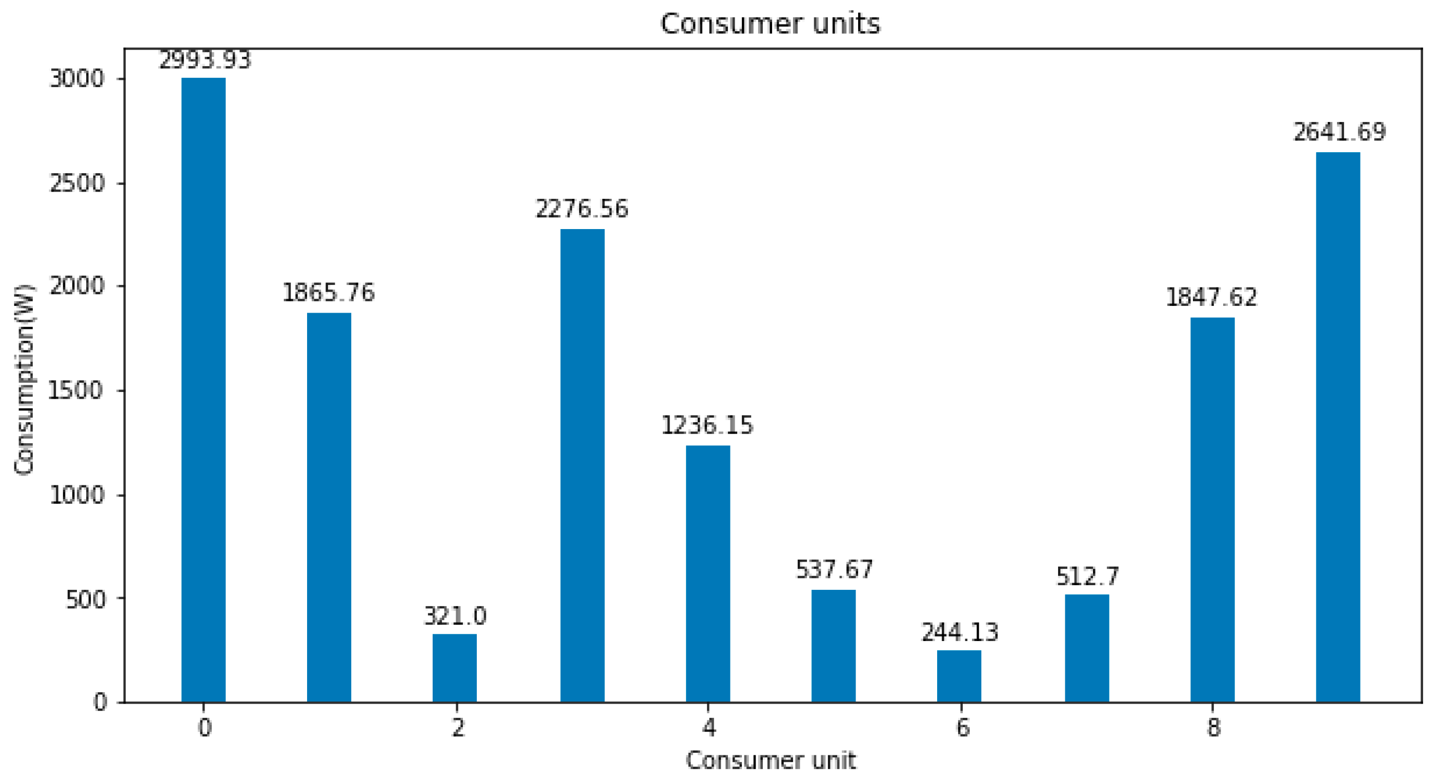
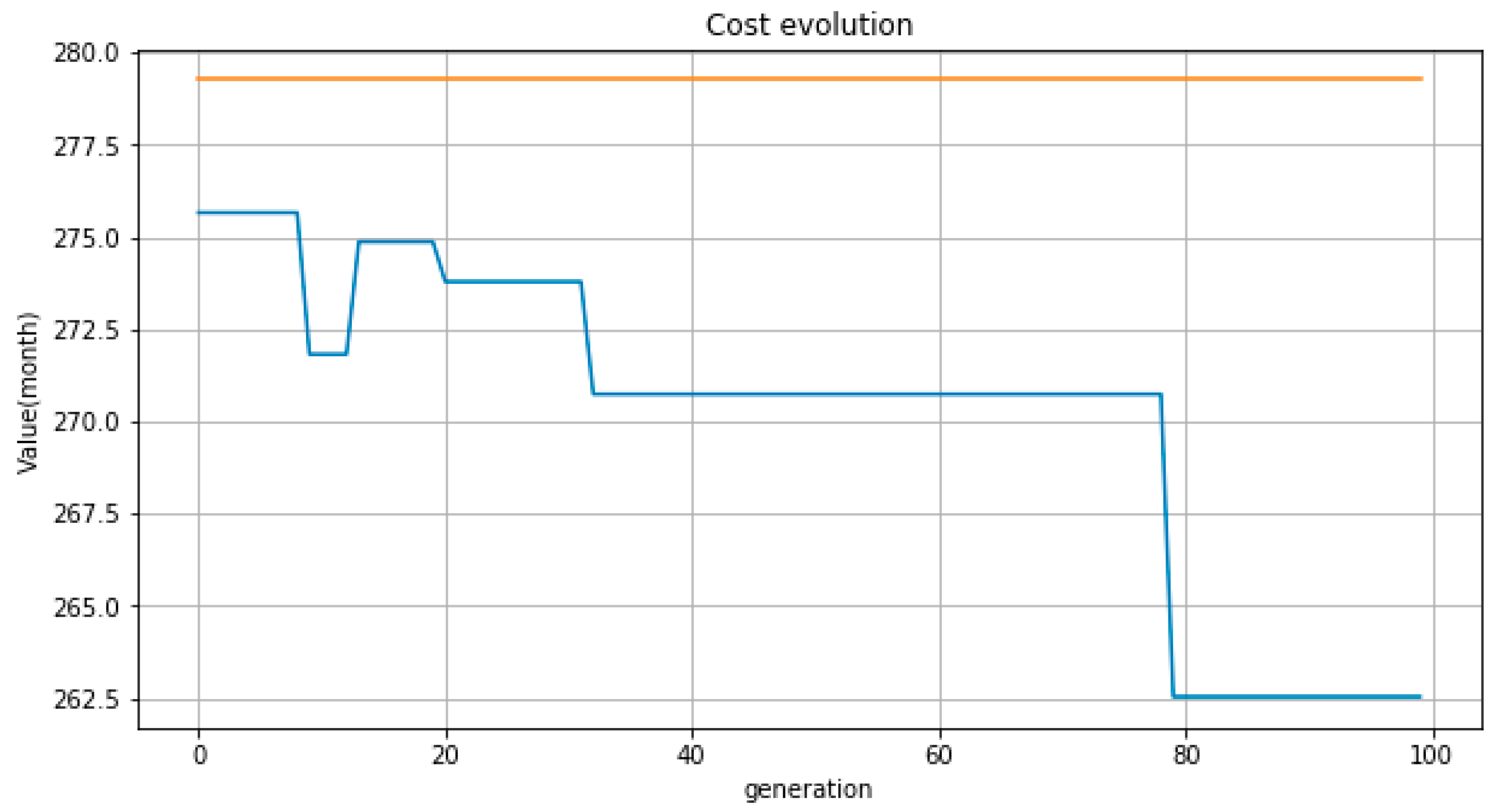
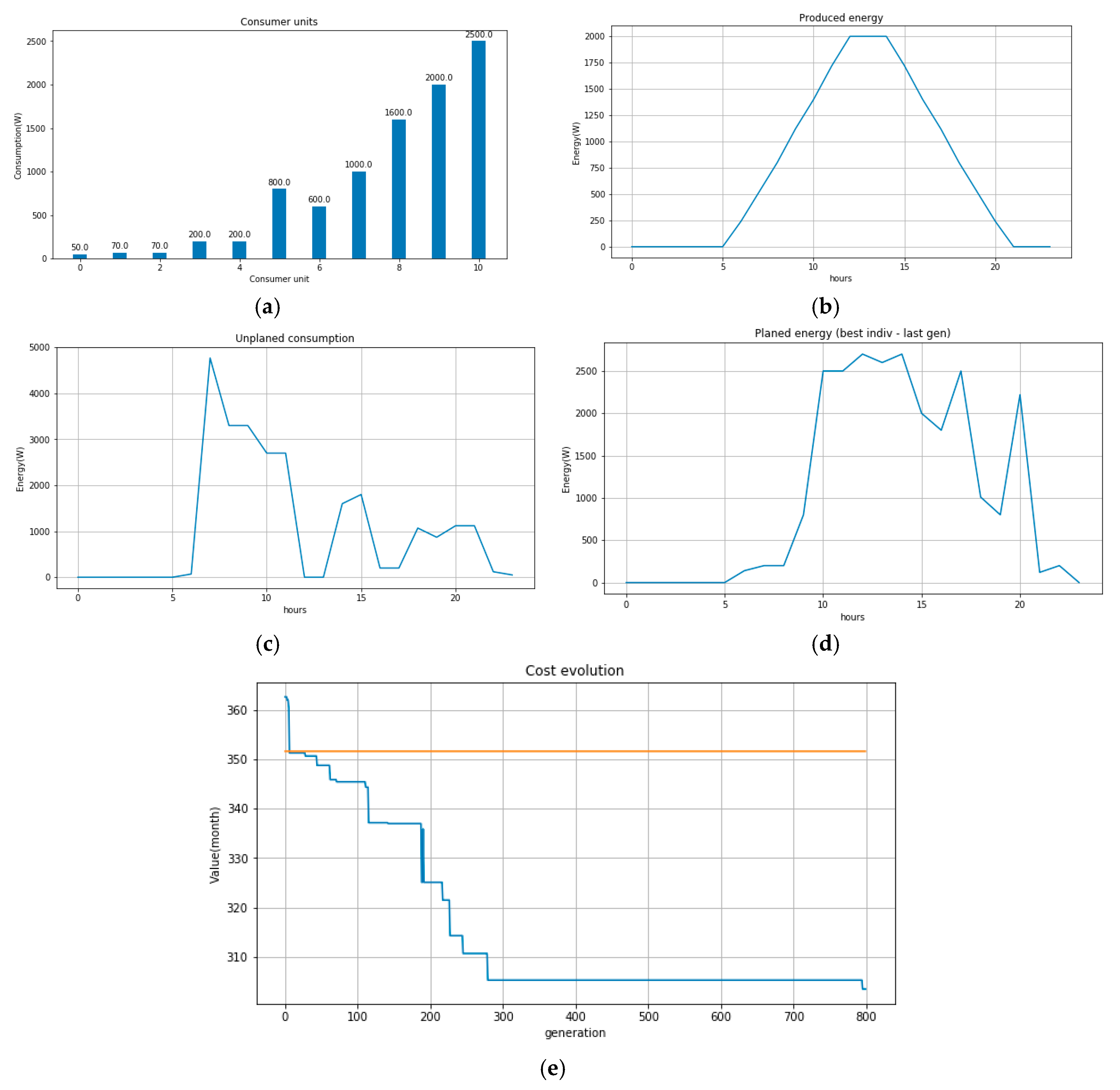
Table 1.
Parameters of genetic algorithm.
| Parameter | Value |
|---|---|
| Population type | Fixed size |
| Population size | 10 individuals |
| Number of generations | 800 |
| Selection | Roulette rule |
| Crossover rate | 1/generation |
| Crossover points | 1 |
| Mutation rate | 0.5/generation |
| Mutation points | 1 |
| Replacement | Offspring from crossover replace individual with weakest evaluation (fitness) |
| Evaluation | CT—see Relation (7) |
| Objective | See Relation (8) |
| Ending criteria | After 800 generations |
Table 2.
Consumer schedule for a profile (case study) generated by simulator.
| Consumer Unit No. | 0 | 1 | 2 | 3 | 4 | 5 | 6 | 7 | 8 | 9 |
|---|---|---|---|---|---|---|---|---|---|---|
| Start time | 2:00 | 3:00 | 19:00 | 4:00 | 13:00 | 14:00 | 20:00 | 15:00 | 18:00 | 22:00 |
| Stop time | 13:00 | 20:00 | 20:00 | 9:00 | 20:00 | 19:00 | 21:00 | 22:00 | 18:00 | 22:00 |
| Number of operations hours per interval | 9 | 4 | 1 | 9 | 1 | 2 | 1 | 2 | 0 | 0 |
Table 3.
Set of parameters from the simulator used for measurements presented below.
| CONSUMERS NO | consMin [W] | consMax [W] | PRODUCER PEAK [W] | SUPPLIER PEAK [W] | SUPPLIER COST RON/W | PRODUCER COST RON/W |
|---|---|---|---|---|---|---|
| 10 | 100 | 3000 | 2000 | 6000 | 0.6/1000 | 0.3/1000 |
Table 4.
Results from a set of profiles generated by the simulator for PRODUCER_COST = 0.3 RON/1000 W.
Table 4.
Results from a set of profiles generated by the simulator for PRODUCER_COST = 0.3 RON/1000 W.
| PRODUCER_PEAK [W] | Measure No. | Range of Cost Decrease between Unplanned and Planned Consumption Schema in Favor of the Planned Consumption [%] | Average Cost Decrease between Unplanned and Planned Consumption Schema in Favor of the Planned Consumption [%] |
|---|---|---|---|
| 2000 | 30 | 3.25–7.14 | 4.81 |
| 3000 | 40 | 5.48–11.59 | 8.95 |
| 4000 | 40 | 2.97–11.24 | 6.55 |
| 5000 | 40 | 7.14–16.11 | 11.48 |
| 6000 | 40 | 5.79–19.51 | 11.90 |
| 7000 | 40 | 8–21.43 | 14.23 |
| 8000 | 30 | 15.38–22.5 | 18.48 |
Table 5.
Results from a set of measurements in which PRODUCER_COST = 0.2 RON/1 kW.
| PRODUCER_PEAK [W] | Measure No. | Range of Decreasing Cost between Unplanned and Planned Consumption Schema [%] | Medium Cost Decrease between Unplanned and Planned Consumption Schema [%] |
|---|---|---|---|
| 2000 | 40 | 3.06–36.54 | 14.15 |
| 3000 | 40 | 2.43–25.78 | 11.14 |
| 4000 | 40 | 7.52–25.39 | 16.45 |
| 5000 | 40 | 6.33–24.02 | 14.21 |
| 6000 | 40 | 19.07–35.71 | 25.33 |
| 7000 | 40 | 5.60–28.83 | 19.50 |
| 8000 | 40 | 16.41–36.49 | 25.65 |
© 2020 by the authors. Licensee MDPI, Basel, Switzerland. This article is an open access article distributed under the terms and conditions of the Creative Commons Attribution (CC BY) license (http://creativecommons.org/licenses/by/4.0/).
Share and Cite
MDPI and ACS Style
Ionescu, L.-M.; Bizon, N.; Mazare, A.-G.; Belu, N. Reducing the Cost of Electricity by Optimizing Real-Time Consumer Planning Using a New Genetic Algorithm-Based Strategy. Mathematics 2020, 8, 1144. https://doi.org/10.3390/math8071144
AMA Style
Ionescu L-M, Bizon N, Mazare A-G, Belu N. Reducing the Cost of Electricity by Optimizing Real-Time Consumer Planning Using a New Genetic Algorithm-Based Strategy. Mathematics. 2020; 8(7):1144. https://doi.org/10.3390/math8071144
Chicago/Turabian StyleIonescu, Laurentiu-Mihai, Nicu Bizon, Alin-Gheorghita Mazare, and Nadia Belu. 2020. "Reducing the Cost of Electricity by Optimizing Real-Time Consumer Planning Using a New Genetic Algorithm-Based Strategy" Mathematics 8, no. 7: 1144. https://doi.org/10.3390/math8071144
Note that from the first issue of 2016, this journal uses article numbers instead of page numbers. See further details here.