1. Introduction
It is easy to observe that large fluctuations in stock market prices are followed by large ones, whereas small fluctuations in prices are more likely to be followed by small ones. This property is known as volatility clustering. Recent works, such as [
1,
2], have shown that while large fluctuations tend to be more clustered than small ones, large losses tend to lump together more severely than large gains. The financial literature is interested in modeling volatility clustering since the latter is considered as a key indicator of market risk. In fact, the trading volume of some assets, such as derivatives, increases over time, making volatility their most important pricing factor.
It is worth mentioning that both, high and low volatilities, seem to be a relevant factor for stock market crises according to Danielsson et al. [
3]. They also found that the relation between unexpected volatility and the incidence of crises became stronger in the last few decades. In the same line, Valentine et al. [
4] showed that market instability is not only the result of large volatility, but also of small volatility.
The classical approach for volatility clusters lies in nonlinear models, based on heteroskedastic conditionally variance. They include ARCH [
5], GARCH [
6,
7,
8], IGARCH [
9], and FIGARCH [
10,
11] models.
On the other hand, agent-based models allow reproducing and explaining some stylized facts of financial markets [
12]. Interestingly, several works have recently been appeared in the literature analyzing a complete order book by real-time simulation [
13,
14,
15]. Regarding the volatility clustering, it is worth mentioning that Lux et al. [
16] highlighted that volatility is explained by market instability. Later, Raberto et al. [
17] introduced an agent-based artificial market whose heterogeneous agents exchange only one asset, which exhibits some key stylized facts of financial markets. They found that the volatility clustering effect is sensitive to the model size, i.e., when the number of operators increases, the volatility clustering effect tends to disappear. That result is in accordance with the concept of market efficiency.
Krawiecki et al. [
18] introduced a microscopic model consisting of many agents with random interactions. Then the volatility clustering phenomenon appears as a result of attractor bubbling. Szabolcs and Farmer [
19] empirically developed a behavioral model for order placement to study endogenous dynamics of liquidity and price formation in the order book. They were able to describe volatility through the order flow parameters.
Alfarano et al. [
20] contributed a simple model of an agent-based artificial market with volatility clustering generated due to interaction between traders. Similar conclusions were obtained by Cont [
21], Chen [
22], He et al. [
23], and Schmitt and Westerhoff [
24].
Other findings on the possible causes of volatility clusters are summarized below. Cont [
21] showed that volatility is explained by agent behavior; Chen [
22] stated that return volatility correlations arise from asymmetric trading and investors’ herding behavior; He et al. [
23] concluded that trade between fundamental noise and noise traders causes the volatility clustering; and Schmitt and Westerhoff [
24] highlighted that volatility clustering arises due to the herding behavior of speculators.
Chen et al. [
25] proposed an agent-based model with multi-level herding to reproduce the volatilities of New York and Hong Kong stocks. Shi et al. [
26] explained volatility clustering through a model of security price dynamics with two kind of participants, namely speculators and fundamental investors. They considered that information arrives randomly to the market, which leads to changes in the viewpoint of the market participants according to a certain ratio. Verma et al. [
27] used a factor model to analyze how market volatility could be explained by assets’ volatility.
An interesting contribution was made by Barde in [
28], where the author compared the performance of this kind of model with respect to the ARCH/GARCH models. In fact, the author remarked that the performance of three kinds of agent-based models for financial markets is better in key events. Population switching was found also as a crucial factor to explain volatility clustering and fat tails.
On the other hand, the concept of a volatility series was introduced in [
2] to study the volatility clusters in the S&P500 series. Moreover, it was shown that the higher the self-similarity exponent of the volatility series of the S&P500, the more frequent the volatility changes and, therefore, the more likely that the volatility clusters appear. In the current article, we provide a novel methodology to calculate the probability of volatility clusters of a given size in a series with special emphasis on cryptocurrencies.
Since the introduction of Bitcoin in 2008, the cryptocurrency market has experienced a constant growth, just like the use of crypto assets as an investment or medium of exchange day to day. As of June 2020, there are 5624 cryptocurrencies, and their market capitalization exceeds 255 billion USD according to the website CoinMarketCap [
29]. However, one of the main characteristics of cryptocurrencies is the high volatility of their exchange rates, and consequently, the high risk associated with their use.
Lately, Bitcoin has received more and more attention by researchers. Compared to the traditional financial markets, the cryptocurrency market is very young, and because of this, there are relatively few research works on their characteristics, and all of them quite recent. Some of the authors analyzed the Bitcoin market efficiency by applying different approaches, including the Hurst exponent (cf. [
30] for a detailed review), whereas others investigated its volatility using other methods. For instance, Letra [
31] used a GARCH model for Bitcoin daily data; Bouoiyour and Selmi [
32] carried out many extensions of GARCH models to estimate Bitcoin price dynamics; Bouri, Azzi, and Dyhberg [
33] analyzed the relation between volatility changes and price returns of Bitcoin based on an asymmetric GARCH model; Balcilar et al. [
34] analyzed the relation between the trading volume of Bitcoin and its returns and volatility by employing, in contrast, a non-parametric causality in quantiles test; and Baur et al. [
35] studied the statistical properties of Bitcoin and its relations with traditional asset classes.
Meanwhile, in 2017, Bariviera et al. [
36] used the Hurst exponent to compare Bitcoin dynamics with standard currencies’ dynamics and detected evidence of persistent volatility and long memory, facts that justify the GARCH-type models’ application to Bitcoin prices. Shortly after that, Phillip et al. [
37] provided evidence of slight leverage effects, volatility clustering, and varied kurtosis. Furthermore, Zhang et al. [
38] analyzed the first eight cryptocurrencies that represent almost
of cryptocurrency market capitalization and pointed out that the returns of cryptocurrencies exhibit leverage effects and strong volatility clustering.
Later, in 2019, Kancs et al. [
39], based on the GARCH model, estimated factors that affect Bitcoin price. For it, they used hourly data for the period between 2013 and 2018. After plotting the data graphically, they suggested that periods of high volatility follow periods of high volatility, and periods of low volatility follow periods of low volatility, so in the series, large returns follow large returns and small returns small returns. All these facts indicate evidence of volatility clustering and, therefore, that the residue is conditionally heteroscedastic.
The structure of this article is as follows. Firstly,
Section 2 contains some mathematical basic concepts on measure theory and probability (
Section 2.1), the FD4 approach
Section 2.2), and the volatility series (
Section 2.3). The core of the current paper is provided in
Section 3, where we explain in detail how to calculate the probability of volatility clusters of a given size. A study of volatility clusters in several cryptocurrencies, as well as in traditional exchanges is carried out in
Section 4. Finally,
Section 5 summarizes the main conclusions of this work.
2. Methods
This section contains some mathematical tools of both measure and probability theories (cf.
Section 2.1) that allow us to mathematically describe the FD4 algorithm applied in this article (cf.
Section 2.2) to calculate the self-similarity index of time series. On the other hand, the concept of a volatility series is addressed in
Section 2.3.
2.1. Random Functions, Their Increments, and Self-Affinity Properties
Let denote time and be a probability space. We shall understand that is a random process (also a random function) from to , if is a random variable for all and , where denotes a sample space. As such, we may think of as defining a sample function for all . Hence, the points in do parameterize the functions with P being a measure of probability in the class of such functions.
Let
and
be two random functions. The notation
means that the finite joint distribution functions of such random functions are the same. A random process
is said to be self-similar if there exists a parameter
such that the following power law holds:
for each
and
. If Equation (
1) is fulfilled, then
H is named the self-similarity exponent (also index) of the process
. On the other hand, the increments of a random function
are said to be stationary as long as
for all
and
. We shall understand that the increments of a random function are self-affine of the parameter
if the next power law stands for all
and
:
Let
be a random function with self-affine increments of the parameter
H. Then, the following
-law holds:
where its (
T-period) cumulative range is defined as:
and
(cf. Corollary 3.6 in [
40]).
2.2. The FD4 Approach
The FD4 approach was first contributed in [
41] to deal with calculations concerning the self-similarity exponent of random processes. It was proven that the FD4 generalizes the GM2 procedure (cf. [
42,
43]), as well as the fractal dimension algorithms (cf. [
44]) to calculate the Hurst exponent of any process with stationary and self-affine increments (cf. Theorem 3.1 in [
41]). Moreover, the accuracy of such an algorithm was analyzed for samples of (fractional) Brownian motions and Lévy stable processes with lengths ranging from
to
points (cf. Section 5 in [
41]).
Next, we mathematically show how that parameter could be calculated by the FD4 procedure. First of all, let
be a random process with stationary increments. Let
, and assume that for each
, there exists
, its (absolute)
q-order moment. Suppose, in addition, that there exists a parameter
for which the next relation, which involves (
-period) cumulative ranges of
, holds:
Recall that this power law stands for the class of (
H-)self-similar processes with self-affine increments (of parameter
H; see
Section 2.1), which, roughly speaking, is equivalent to the class of processes with stationary increments (cf. Lemma 1.7.2 in [
45]). Let us discretize the period by
and take
q-powers on both sides of Equation (
2). Thus, we have:
Clearly, the expression in Equation (
3) could be rewritten in the following terms:
where, for short, the notation
is used for all
. Since the two random variables in Equation (
4) are equally distributed, their means must be the same, i.e.,
Taking (2-base) logarithms on both sides of Equation (
5), the parameter
H could be obtained by carrying out a linear regression of:
vs.
q. Alternatively, observe that the expression in Equation (
4) also provides a relation between cumulative ranges of consecutive periods of
, i.e.,
Since the random variables on each side of Equation (
7) have the same (joint) distribution function, their means must be equal, namely,
which provides a strong connection between consecutive moments of order
q of
. If (two-base) logarithms are taken on both sides of Equation (
8), a linear regression of the expression appearing in Equation (
9) vs.
q allows calculating the self-similarity exponent of
(whenever self-similar patterns do exist for such a process):
Hence, the FD algorithm is defined as the approach whose running is based on the expressions appearing in either Equation (
5) or Equation (
8). The main restriction underlying the FD algorithm consists of the assumption regarding the existence of the
q-order moments of the random process
. At first glance, any non-zero value could be assigned to
q to calculate the self-similarity exponent (provided that the existence of that sample moment could be guaranteed). In the case of Lévy stable motions, for example, given
, it may occur that
does not exist for any
. As such, we shall select
to calculate the self-similarity index of a time series by the FD algorithm, thus leading to the so-called FD4 algorithm. Equivalently, the FD4 approach denotes the FD algorithm for
. In this paper, the self-similarity exponent of a series by the FD4 approach is calculated according to the expression in Equation (
6). Indeed, since it is equivalent to:
the Hurst exponent of the series is obtained as the slope of a linear regression, which compares
with respect to
n. In addition, notice that a regression coefficient close to one means that the expression in Equation (
5) is fulfilled. As such, the calculation of
becomes necessary to deal with the procedure described above, and for each
n, it depends on a given sample of the random variable
. For computational purposes, the length of any sample of
is chosen to be equal to
. Accordingly, the greater
n, the more accurate the value of
is. Next, we explain how to calculate
. Let a log-price series be given, and divide it into
non-overlapping blocks,
. The length of each block is
, so for each
, we can write
. Then:
Determine the range of each block , i.e., calculate for each .
The (q-order) sample moment is given by .
According to the step (1), both the minimum and the maximum values of each period are required to calculate each range . In this way, notice that such values are usually known for each trading period in the context of financial series. It is also worth noting that when n takes the value , then each block only consists of a single element. In this case, though, each range can be still computed.
2.3. The Volatility Series
The concept of a volatility series was first contributed in Section 2.2 of [
2] as an alternative to classical (G)ARCH models with the aim to detect volatility clusters in series of asset returns from the S&P500 index. It was found, interestingly, that whether clusters of high (resp., low) volatility appear in the series, then the self-similarity exponent of the associated volatility series increases (resp., decreases).
Let denote the log-return series of a (index/stock) series. In financial series, the autocorrelation function of the ’s is almost null, though the series is not. The associated volatility series is defined as , where refers to the absolute value function, m is a constant, and . For practical purposes, we set .
Next, we explain how the Hurst exponent of the volatility series,
, could provide a useful tool to detect volatility clusters in a series of asset returns. Firstly, assume that the volatility of the series is constant. Then, the values of the associated volatility series would be similar to those from a sample of a Brownian motion. Hence, the self-similarity exponent of that volatility series would become close to
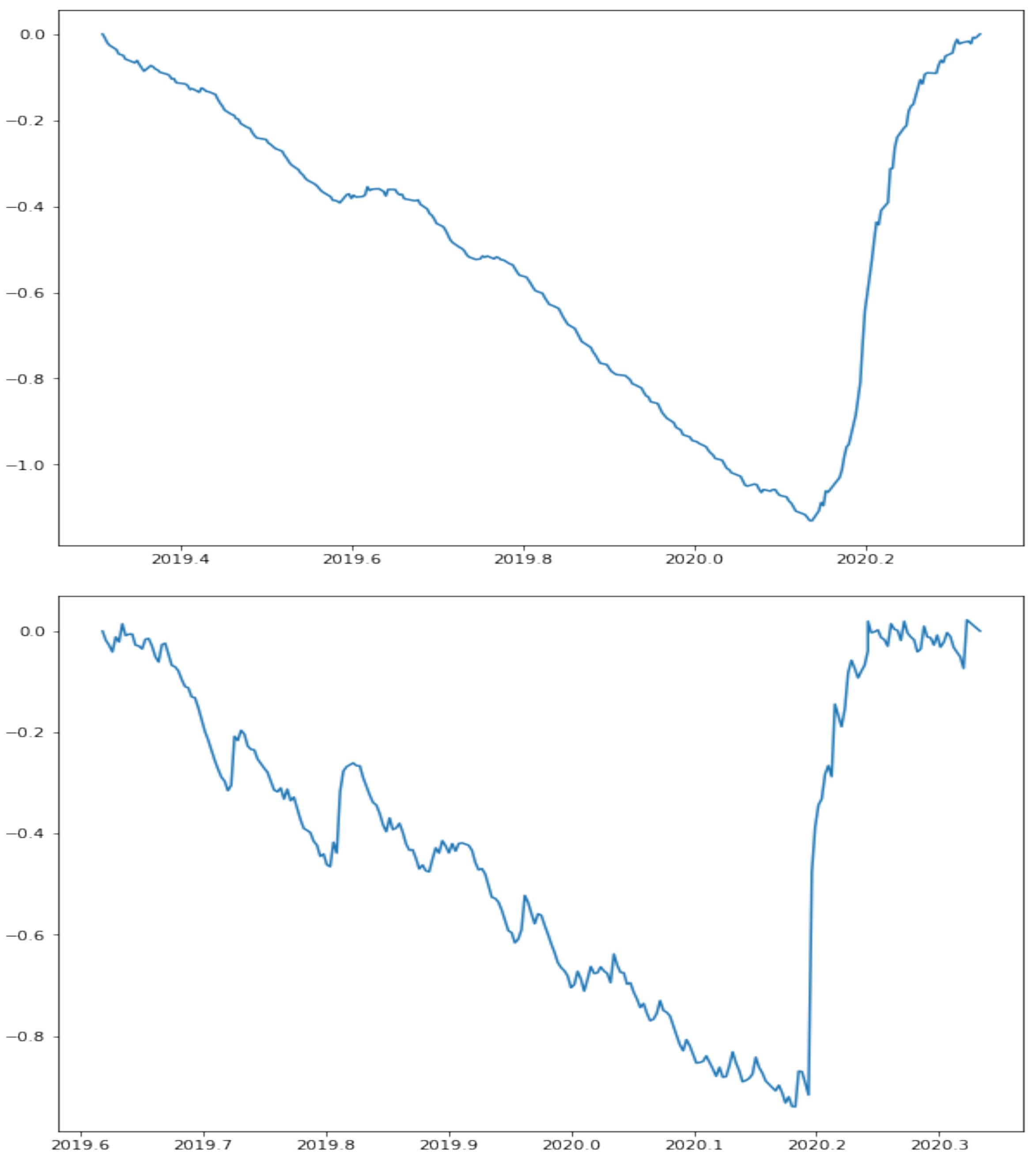
. On the contrary, suppose that there exist some clusters of high (resp., low) volatility in the series. Thus, the graph of its associated volatility series becomes smoother, as illustrated in
Figure 1, which also depicts the concept of a volatility series. Hence, almost all the values of the volatility series are greater (resp., lower) than the mean of the series. Accordingly, the volatility series turns out to be increasing (resp., decreasing), so its self-similarity exponent also increases (resp., decreases).
Following the above, the Hurst exponent of the volatility series of an index or asset provides a novel approach to explore the presence of volatility clusters in series of asset returns.
3. Calculating the Probability of Volatility Clusters of a Given Size
In this section, we explore how to estimate the probability of the existence of volatility clusters for blocks of a given size. Equivalently, we shall address the next question: What is the probability that a volatility cluster appears in a period of a given size? Next, we show that the Hurst exponent of a volatility series (see
Section 2.2 and
Section 2.3) for blocks of that size plays a key role.
We know that the Hurst exponent of the volatility series is high when there are volatility clusters in the series [
2]. However, how high should it be?
To deal with this, we shall assume that the series of (log-)returns follows a Gaussian distribution. However, it cannot be an i.i.d. process since the standard deviation of the Gaussian distribution is allowed to change. This hypothesis is more general than an ARCH or GARCH model, for example. Since we are interested in the real possibility that the volatility changes and, in fact, there exist volatility clusters, a static fixed distribution cannot be assumed. In this way, it is worth noting that the return distribution of these kinds of processes (generated from Gaussian distributions with different standard deviations) is not Gaussian, and it is flexible enough to allow very different kinds of distributions.
As such, let us assume that the series of the log-returns,
, follows a normal distribution,
, where its standard deviation varies over time via the function
. In fact, some classical models such as ARCH, GARCH, etc., stand as particular cases of that model. As such, we shall analyze the existence of volatility clusters in the following terms. We consider that there exist volatility clusters as long as there are, at least, both, a period of high volatility and a period of low volatility.
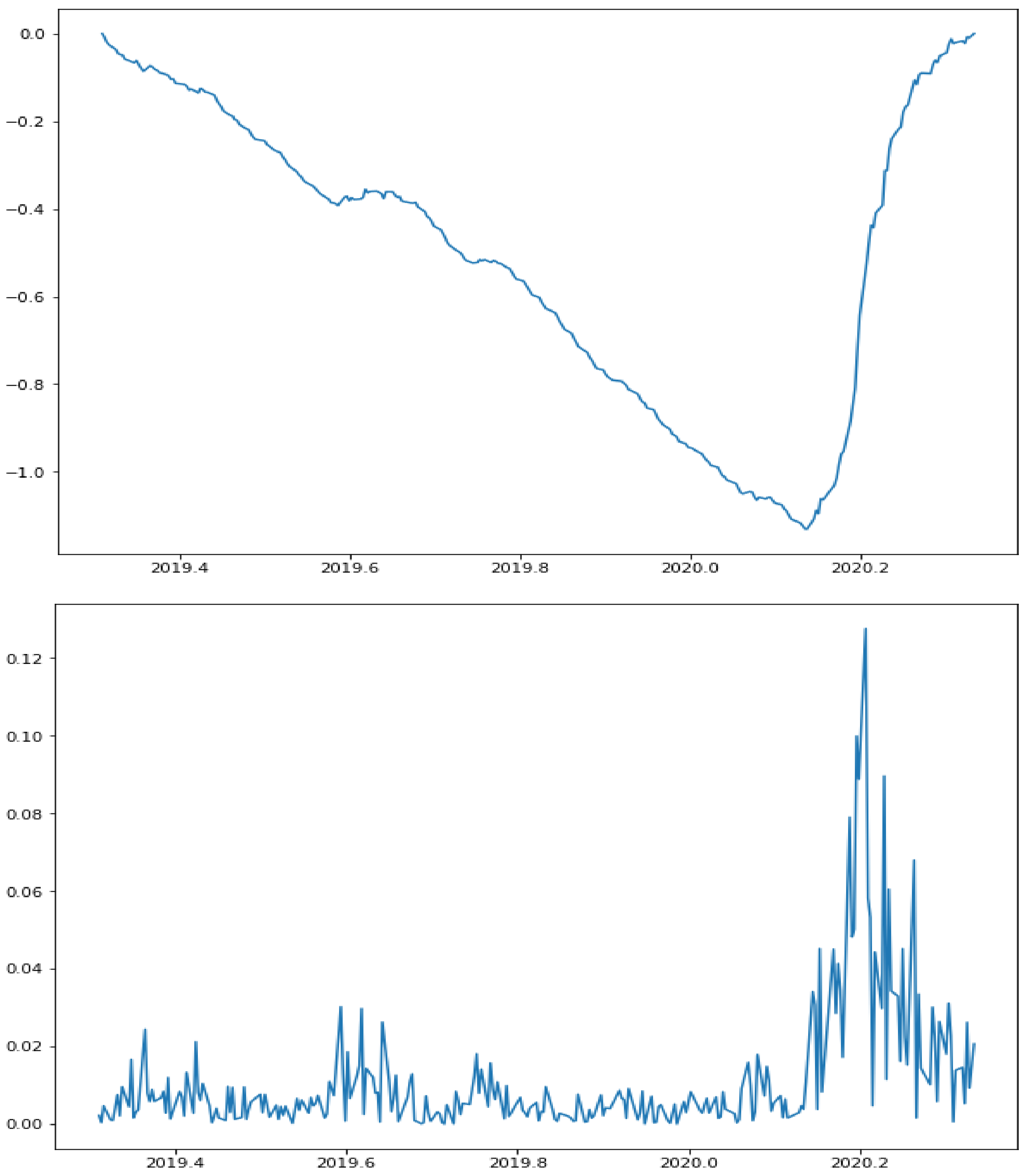
Figure 2 illustrates that condition. Indeed, two broad periods could be observed concerning the volatility series of the S&P500 index. The first one has a low volatility (and hence, a decreasing volatility series) and the second one a high volatility (and hence, an increasing volatility series). In this case, the effect of the higher volatility (due to the COVID-19 crisis) is evident, thus being confirmed by a very high Hurst exponent of the corresponding volatility series (equal to
).
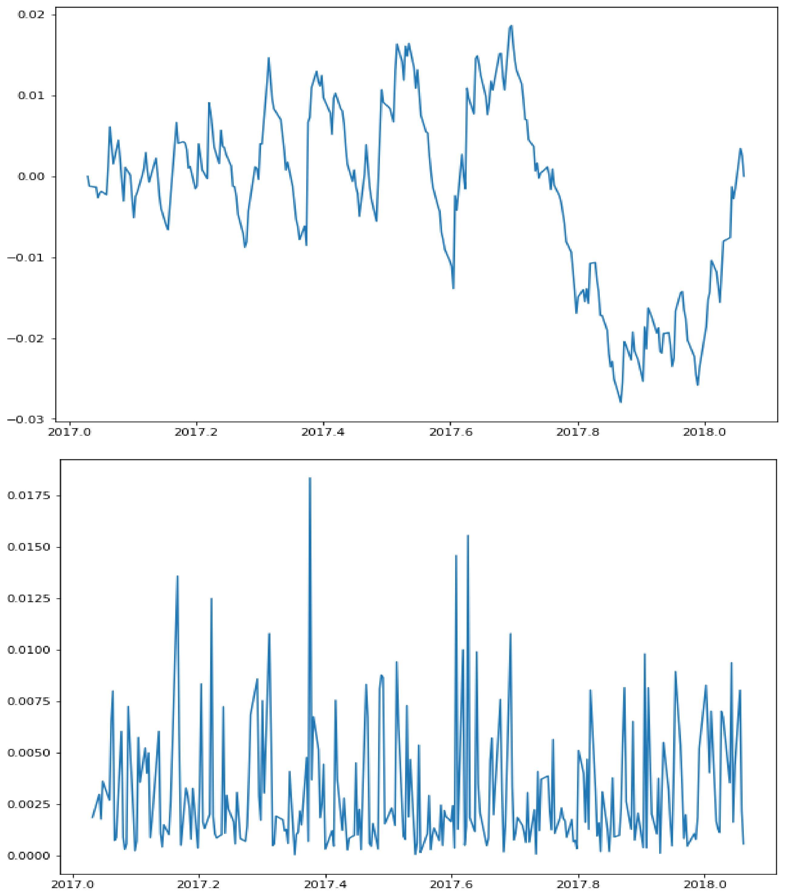
On the other hand,
Figure 3 depicts the volatility series of the S&P500 index in the period ranging from January 2017 to January 2018. A self-similarity index equal to
was found by the FD4 algorithm. In this case, though, it is not so clear that there are volatility clusters, which is in accordance with the low Hurst exponent of that volatility series.
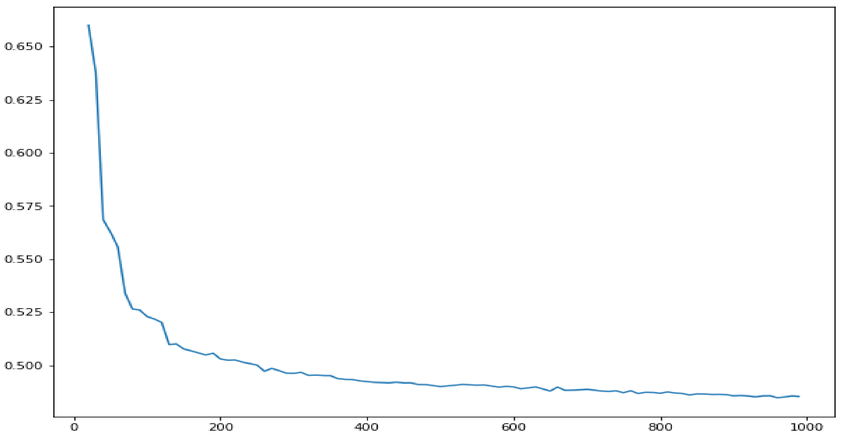
As such, the Hurst exponent of the volatility series of a Brownian motion will be considered as a benchmark in order to decide whether there are volatility clusters in the series. More precisely, first, by Monte Carlo simulation, a collection of Brownian motions was generated. For each Brownian motion, the Hurst exponents (by FD4 approach) of their corresponding volatility series were calculated. Hence, we denote by
the value that becomes greater than
of those Hurst exponents. Observe that
depends on
n, the length of the Brownian motion sample. In fact, for a short series, the accuracy of the FD4 algorithm to calculate the Hurst exponent is lower. Accordingly, the value of
will be higher for a lower value of
n.
Figure 4 illustrates (for the 90th percentile) how the benchmark given by
becomes lower as the length of the Brownian motion series increases.
Therefore, we will use the following criteria. We say that there are volatility clusters in the series provided that the Hurst exponent of the corresponding volatility series is greater than . Then, we will measure the probability of volatility clusters for subseries of a given length as the ratio between the number of subseries with volatility clusters to the total amount of subseries of the given length.
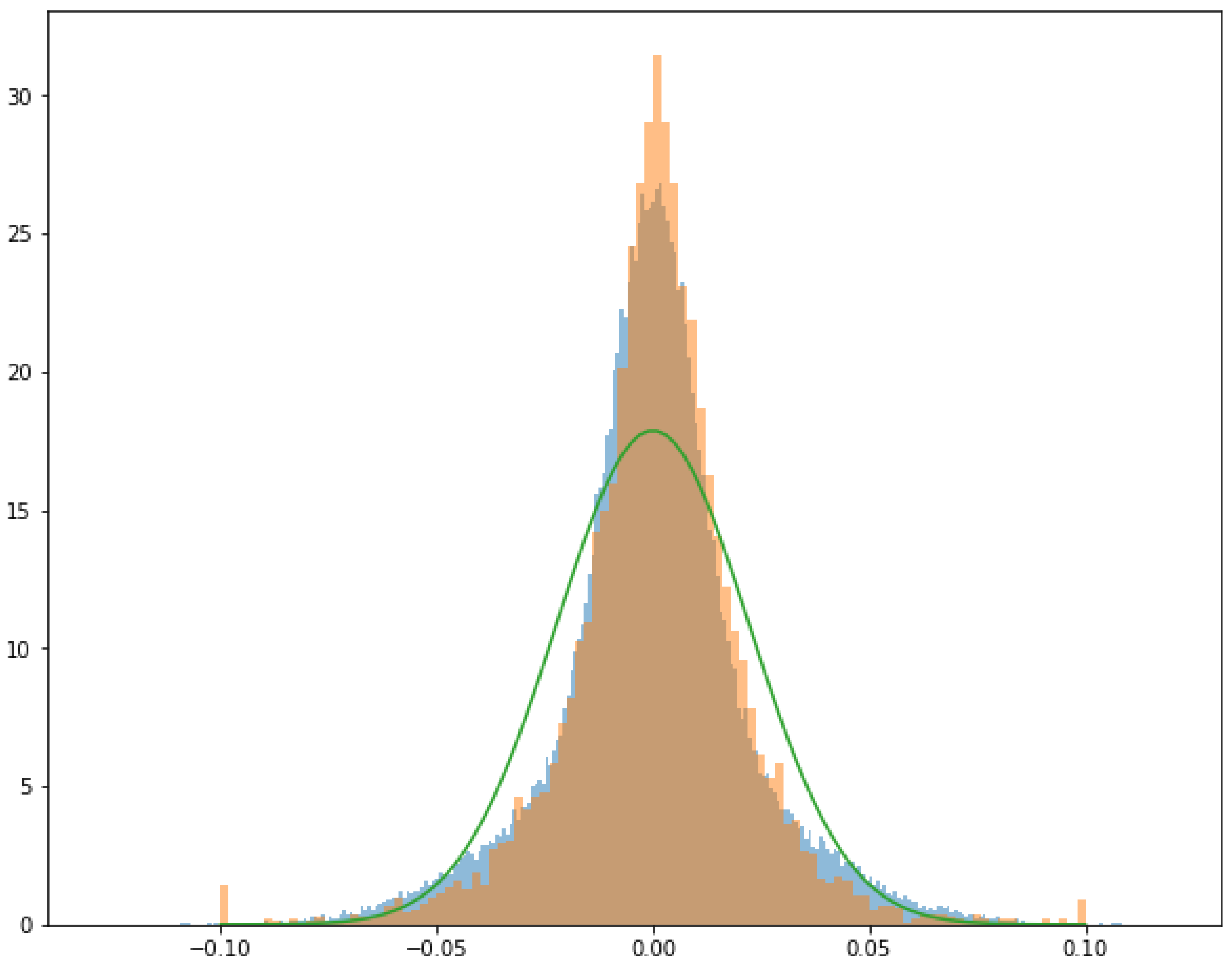
In order to check that measure of the probability of volatility clusters, we will test it by artificial processes with volatility clusters of a fixed length (equal to 200 data). A sample from that process is generated as follows. For the first 200 data, generate a sample from a normal distribution
; for the next 200 data, generate a sample from a normal distribution
; for the next 200 data, generate a sample from a normal distribution
, and so on. It is worth pointing out that a mixture of (samples from) normal distributions with distinct standard deviations can lead to (a sample from) a heavy-tailed distribution. Following that example,
Figure 5 depicts the distribution of that artificial process with volatility clusters compared to the one from a Gaussian distribution and also to the S&P500 return distribution (rescaled). It is clear that the process is far from Gaussian even in that easy example.
For that process, consider one random block of length 50. It may happen that such a block fully lies in a 200 block of fixed volatility. In this case, there will be no volatility clusters. However, if the first 20 data lie in a block of volatility equal to , with the remaining 30 data lying in a block of volatility equal to , then such a block will have volatility clusters. On the other hand, it is clear that if we have one block of length 50 with the first 49 data lying in a block of volatility equal to , whereas the remaining one datum lies in a block of volatility, we cannot say that there are volatility clusters in such a block. Therefore, we shall consider that there are volatility clusters if there are at least 10 data in blocks with distinct volatilities. In other words, we shall assume that we cannot detect clusters with less that 10 data.
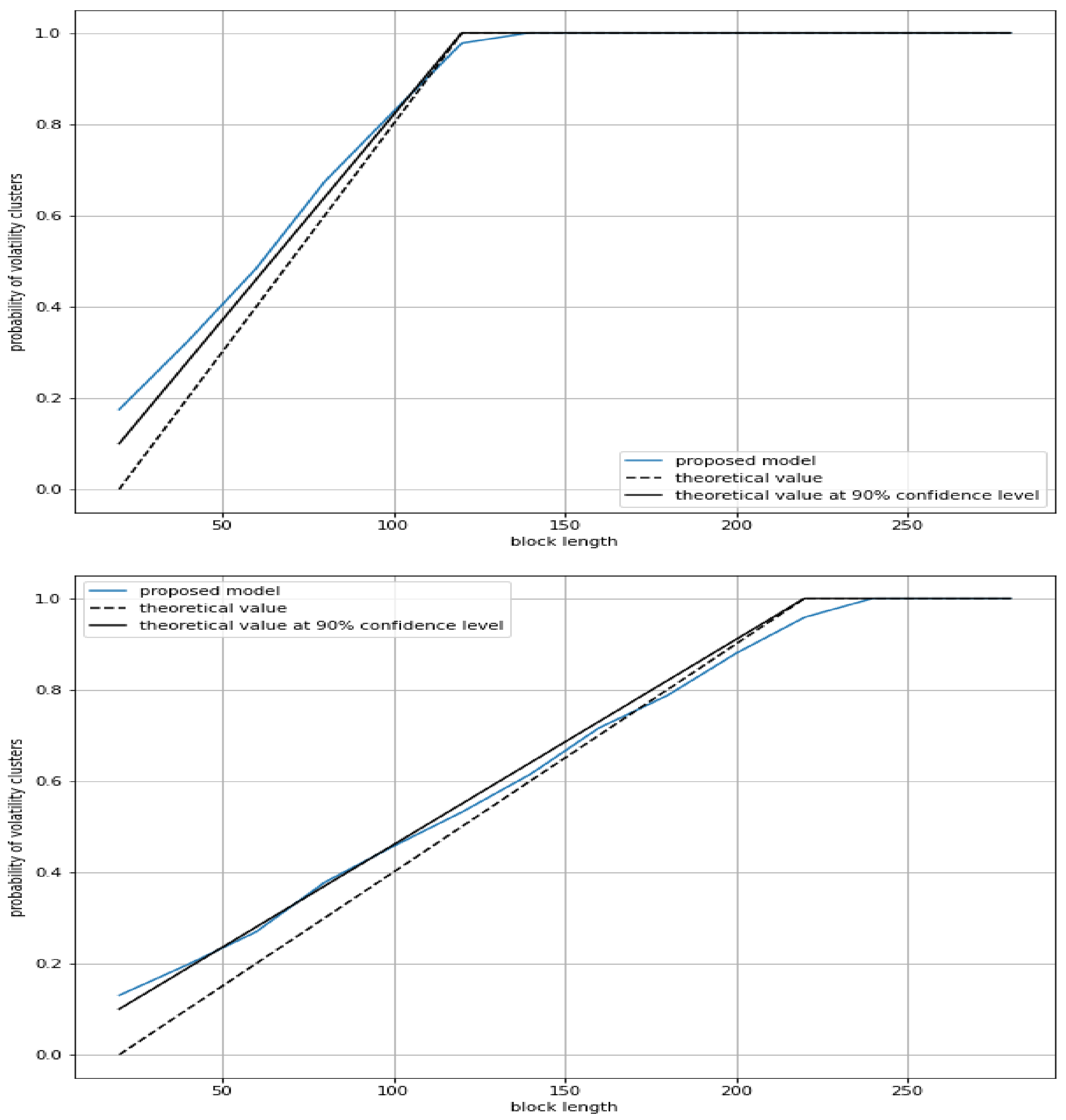
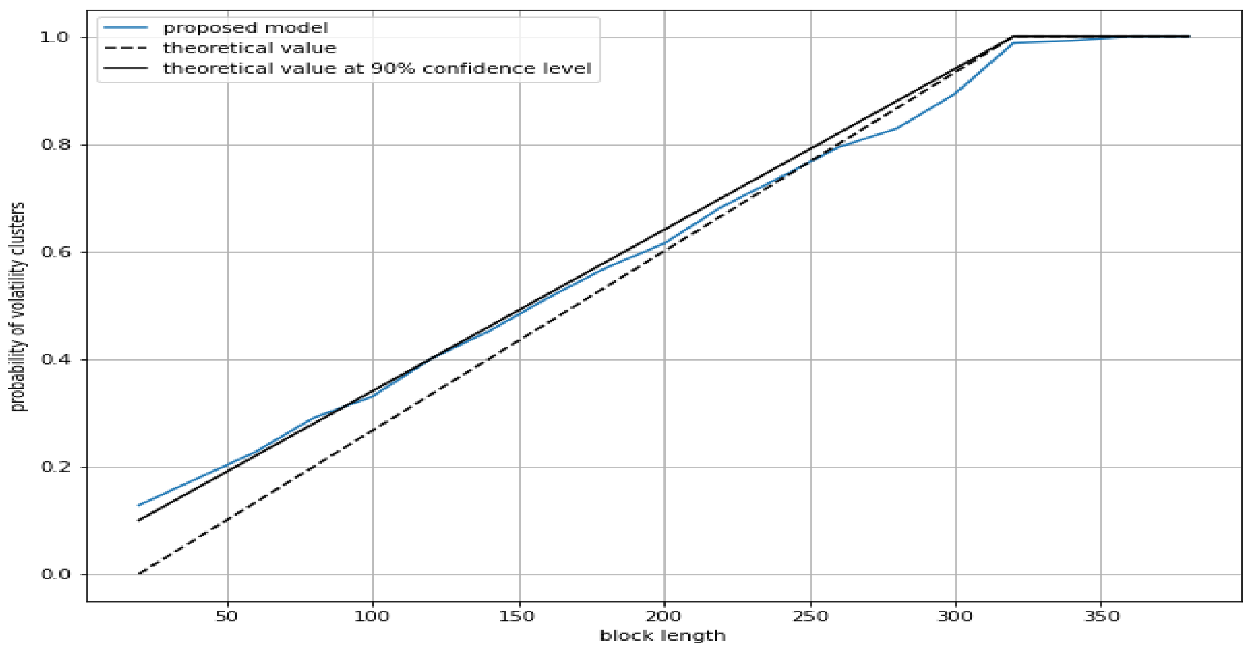
On the other hand, note that we are using a confidence level of , and hence, if we get a probability of volatility clusters of, say, , that means that there are no volatility clusters regarding the of the blocks of the given size. However, for that confidence level of , we are missing of that , and hence, we will have the following theoretical estimates.
Theoretical probability of volatility clusters considering clusters of at least 10 data: .
Theoretical probability of volatility clusters considering clusters of at least 10 data detected at a confidence level of : .
Figure 6 graphically shows that the proposed model for estimating the probability of volatility clusters could provide a fair approximation to the actual probability of volatility clusters for such an artificial process.
5. Conclusions
One of the main characteristics of cryptocurrencies is the high volatility of their exchange rates. In a previous work, the authors found that a process with volatility clusters displays a volatility series with a high Hurst exponent [
2].
In this paper, we provide a novel methodology to calculate the probability of the volatility clusters of a series using the Hurst exponent of its associated volatility series. Our approach, which generalizes the (G)ARCH models, was tested for a class of processes artificially generated with volatility clusters of a given size. In addition, we provided an explicit criterion to computationally determine whether there exist volatility clusters of a fixed size. Interestingly, this criterion is in line with the behavior of the Hurst exponent (calculated by the FD4 approach) of the corresponding volatility series.
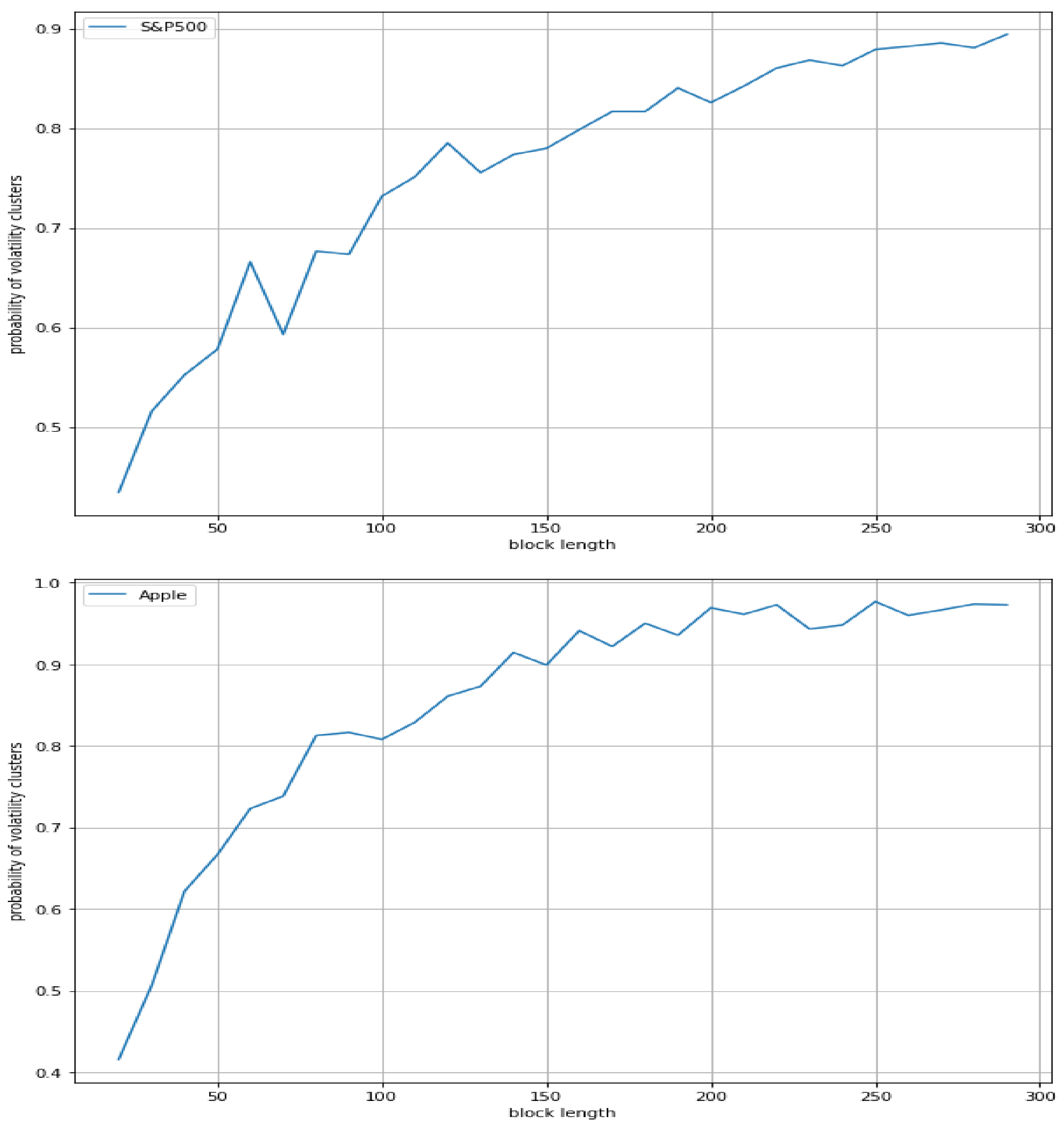
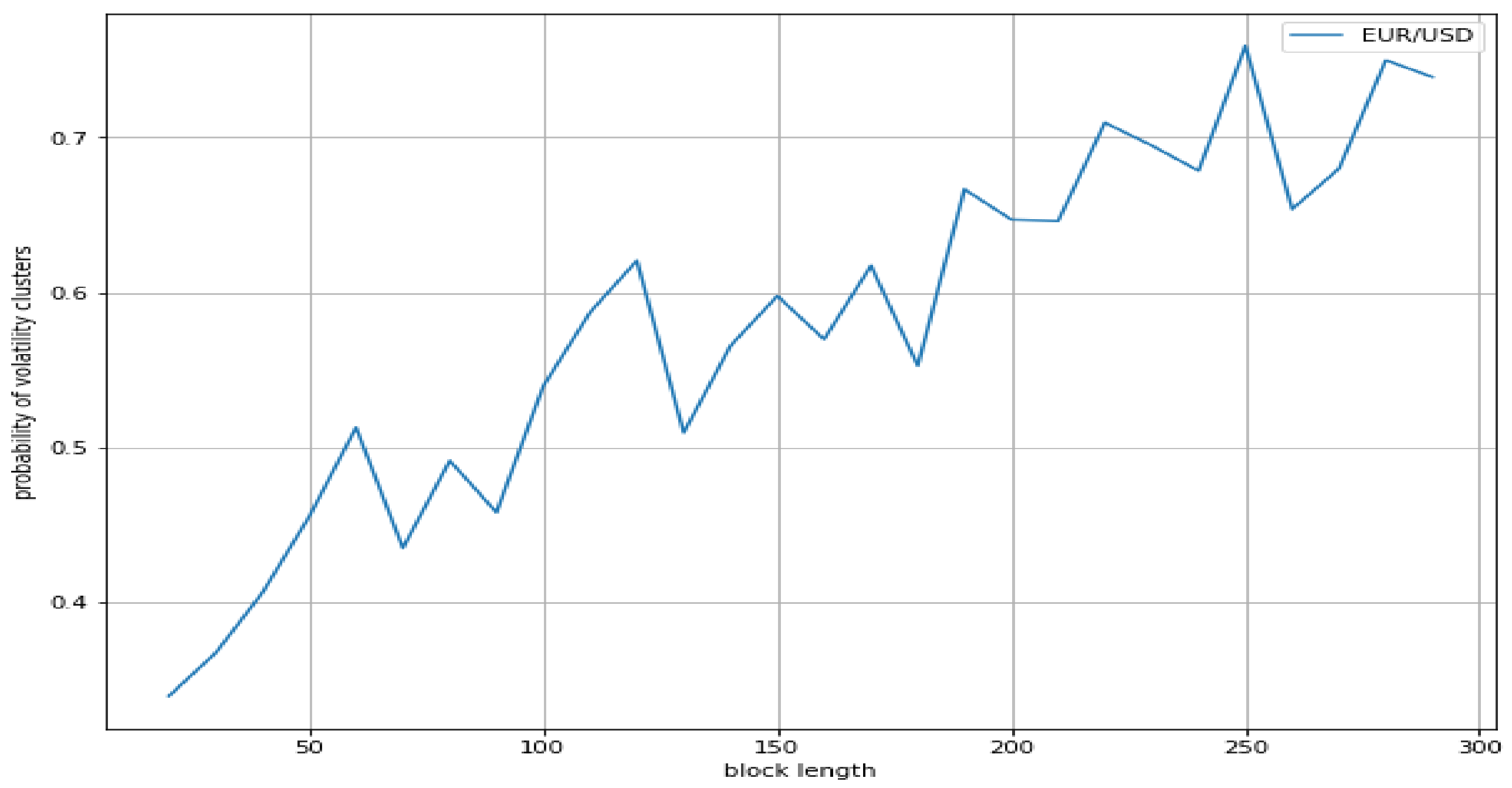
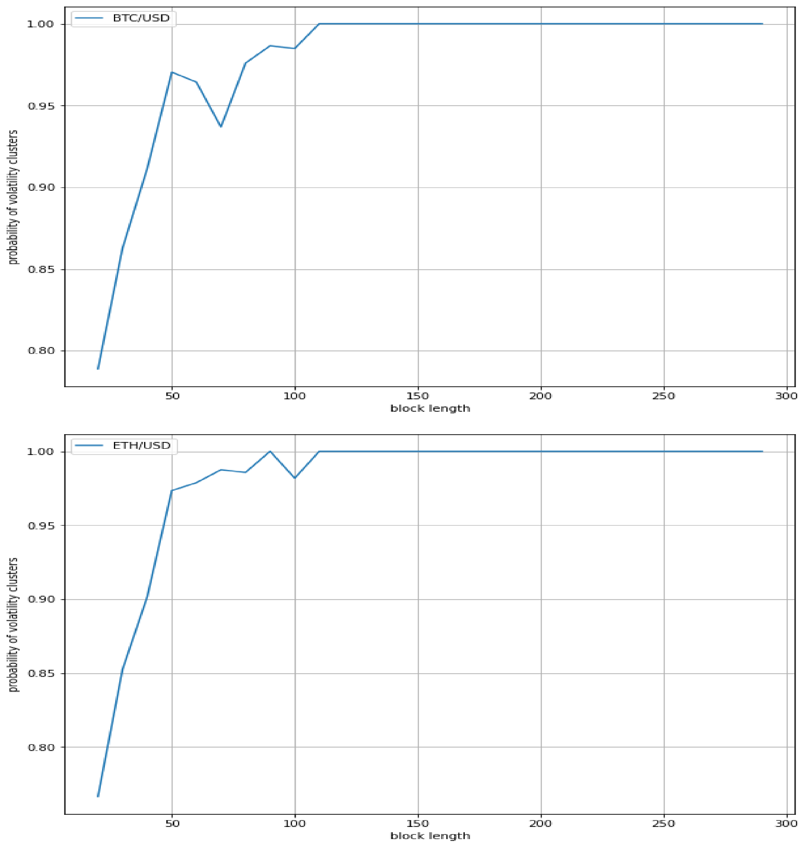
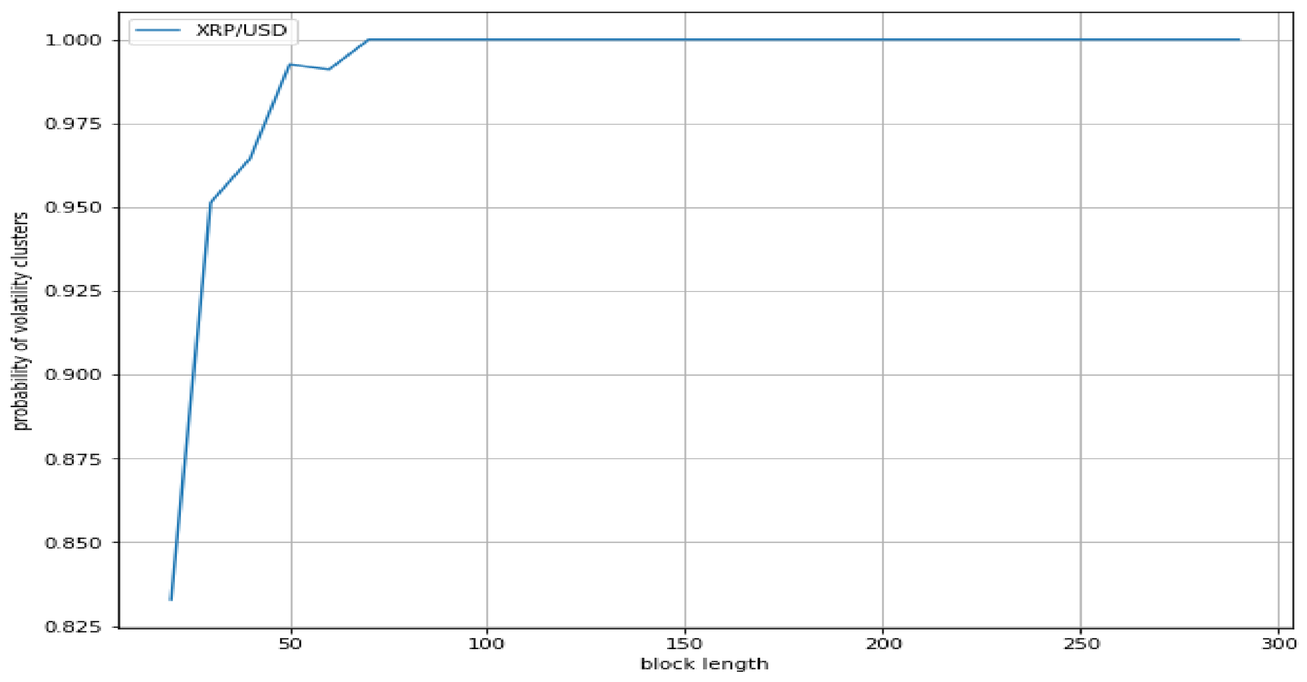
We found that the probabilities of volatility clusters of an index (S&P500) and a stock (Apple) show a similar profile, whereas the probability of volatility clusters of a forex pair (Euro/USD) results in being quite lower. On the other hand, a similar profile appears for Bitcoin/USD, Ethereum/USD, and Ripple/USD cryptocurrencies, with the probabilities of volatility clusters of all such cryptocurrencies being much greater than the ones of the three traditional assets. Accordingly, our results suggest that the volatility in cryptocurrencies changes faster than in traditional assets, and much faster than in forex pairs.


 ,
, 


