Radiative MHD Sutterby Nanofluid Flow Past a Moving Sheet: Scaling Group Analysis
by
 , , , and
Mohammed M. Fayyadh
1 ,
,
Kohilavani Naganthran
2 ,
,
Md Faisal Md Basir
3,
Ishak Hashim
2,* and
Rozaini Roslan
1 1
Department of Mathematics and Statistics, Faculty of Applied Science & Technology, Universiti Tun Hussein Onn Malaysia, Pagoh 86400, Malaysia
2
Department of Mathematical Sciences, Faculty of Science & Technology, Universiti Kebangsaan Malaysia, UKM Bangi 43600, Malaysia
3
Department of Mathematical Sciences, Faculty of Science, Universiti Teknologi Malaysia, UTM Johor Bahru 81310, Malaysia
*
Author to whom correspondence should be addressed.
Mathematics 2020, 8(9), 1430; https://doi.org/10.3390/math8091430
Submission received: 20 July 2020
/
Revised: 21 August 2020
/
Accepted: 24 August 2020
/
Published: 26 August 2020
(This article belongs to the Special Issue Computational Fluid Dynamics 2020)
Abstract
:The present theoretical work endeavors to solve the Sutterby nanofluid flow and heat transfer problem over a permeable moving sheet, together with the presence of thermal radiation and magnetohydrodynamics (MHD). The fluid flow and heat transfer features near the stagnation region are considered. A new form of similarity transformations is introduced through scaling group analysis to simplify the governing boundary layer equations, which then eases the computational process in the MATLAB bvp4c function. The variation in the values of the governing parameters yields two different numerical solutions. One of the solutions is stable and physically reliable, while the other solution is unstable and is associated with flow separation. An increased effect of the thermal radiation improves the rate of convective heat transfer past the permeable shrinking sheet.
1. Introduction
The viscoelastic fluid is a type of non-Newtonian fluid that manifests the viscous and elasticity features under deformation. Sutterby fluid is an example of the viscoelastic fluid, and it well portrays the dilute polymer solutions [1,2]. Specifically, the Sutterby model fluid resembles the shear thinning and shear thickening aspects in high polymer aqueous solutions such as carboxymethyl cellulose (CMC), hydroxyethyl cellulose (HEC) and methyl cellulose (MC) [3]. The dilute polymer solutions have a wide range of functions in industrial practice, for instance, spray applications of agricultural chemicals [4], drag reducers in pipe flows [5], and production of domestic cleaning products [6]. The work of Fujii et al. [7] is one of the earliest studies to address the natural convection boundary layer flow in a Sutterby fluid past a vertical motionless isothermal plane and achieved an excellent comparison with the experimental results. Fujii et al. [8] revisited their work in [7] to investigate the impact of uniform heat flux under the same settings. However, the Sutterby model fluid received less attention from the boundary layer researchers at that time. Later, a new type of heat conductive fluid was introduced by Choi [9] named nanofluid. Nanofluid was also claimed to be a brilliant fluid due to its excellent heat transfer performance in engineering applications such as cooling of electronic appliances, and systems of solar water heating [10]. Nanofluid has now attracted significant interest from researchers, and boundary layer models have been studied under various settings [11,12,13]. After a long discontinuity in the theoretical works of the Sutterby boundary layer fluid flow, some numerical investigations of the Sutterby fluid under the Cattaneo–Christov heat flux [14,15], Soret and Dufour effect [16], peristaltic flow [17,18,19], squeezed flow [20], Joule heating effect [21], homogeneous–heterogeneous reactions [22], and hybrid nanoparticles [23] have been reported recently.
Magnetohydrodynamics (MHD) is another technological conception that is widespread in engineering practice. Electromagnetic casting [24], plasma confinement, and MHD power generation [25] are examples of notable applications. Thermal radiation is a type of energy that works in conjunction with the MHD effect. Thermal radiation emits and absorbs energy in the form of waves or molecules through a non-scattering medium. The successful combination of thermal radiation and MHD in an electrically conducting fluid has significant applications in solar power technology and electrical power generation [26]. Acknowledging these applications, researchers began to examine thermal radiation and MHD effects in the boundary layer flow past a stretching/shrinking surface, and many theoretical works have been reported. Recently, Sabir et al. [27] explored the stagnation-point flow of a Sutterby fluid with the effects of an inclined magnetic field and thermal radiation past a stretching surface, and observed the declining trend of the convective heat transfer with the stronger influence of thermal radiation. Bilal et al. [28] examined the ohmically dissipated Darcy–Forchheimer slip flow of an MHD Sutterby fluid past a radiating stretching sheet and found a decrement in the convective heat transfer with increasing slip effects.
By comparison, the boundary layer equations, which were proposed by Prandtl [29], disclosed many invariant closed-form solutions. Prandtl’s boundary layer equations can be reduced to a less complicated form that is in a system of ordinary differential equations. These boundary layer equations also allow many different types of symmetry groups, of which the Lie group analysis is prominent. Lie group analysis helps to identify the transformation point that represents the given boundary layer equations [30]. In Lie group analysis, the group-invariant solutions are the similarity solutions, and these similarity solutions are used to reduce the independent variables in a fluid flow problem [31]. A special form of the Lie group analysis exists, namely, the scaling group of transformation, and this has been employed by researchers in valuable contributions, for instance, see [32,33].
Regarding studies of stagnation-point flow in a Sutterby fluid, Azhar et al. [34] investigated the effect of entropy generation on the stagnation-point flow of a Sutterby nanofluid past a stretching sheet. Azhar et al. [35] reconsidered the work of [34] by incorporating the Cattaneo–Christov heat flux model and omitting the nanoparticles. Both of the studies of [34,35] solved the flow problem numerically and presented unique solutions. A number of considerable research gaps were found in the theoretical works available in the stagnation-point flow and heat transfer in a Sutterby nanofluid, for instance: inspecting fluid flow behavior and heat transfer characteristics past a shrinking sheet together with the suction effect; conducting scaling group analysis; obtaining dual solutions; and performing stability analysis. Thus, the present work is devoted to numerically solving the problem of boundary layer Sutterby nanofluid flow and heat transfer near the stagnation region over a permeable moving (stretching/shrinking) sheet. The fluid flow and heat transfer characteristics under the magnetic and thermal radiation effects are observed. Scaling group analysis is employed to obtain the apt similarity transformations so that the complex governing boundary layer equations can be brought to a soluble form. The simplified form of the mathematical model is then solved numerically in the boundary value problem solver or bvp4c function in MATLAB. Two different numerical solutions are identified with the governing parameters’ variation. Further, stability analysis is undertaken in the present work to justify the presence of dual solutions. These contributions are essentially original, and all numerical results are presented and discussed in detail.
2. Problem Formulation
Contemplate an incompressible two-dimensional stagnation-point flow of a Sutterby nanofluid across a stretching/shrinking sheet as shown in Figure 1, where x and y are the Cartesian coordinates with the x-axis positioned in the horizontal direction, and the y-coordinate is normal to the x-coordinate. The free stream velocity is denoted by and signifies the velocity of the moving sheet, where infers the state of the stretching sheet, the embodies shrinking sheet, and typifies the stationary sheet. The moving (stretching or shrinking) sheet is penetrable and there is a uniform surface mass flux, of velocity with to imply the injection situation and for the suction state. The free stream temperature and the wall temperature are denoted by and respectively.
Sutterby [1,2] introduced the constitutive law for the Sutterby fluid by expressing the Cauchy stress tensor as:
where is the pressure, is the identity vector, and is the extra stress tensor which can be defined as follows [21]:
Here, is the viscosity at low shear rates, is the material time constant, is the second invariant strain tensor, is the first order Rivlin–Erickson tensor or deformation rate tensor which is defined as and is the power-law index. The Sutterby model in Equation (2) is a versatile model when the value of changes. For instance, when the Sutterby model imitates the Newtonian fluid behavior, when the model is reduced to the Eyring model, and this model also predicts specifically the pseudo-plastic (shear thinning) and dilatant (shear thickening) fluid properties when and respectively. By taking the velocity field as and under the assumptions mentioned earlier, the governing boundary layer equations in the dimensional form can be formed as follows [36]:
along with the respective boundary conditions:
where and denote velocity components in the and directions, respectively, is the dynamic viscosity of the nanofluid, is the electrical conductivity, is the magnetic field strength, is the density of the nanofluid, is the Stefan Boltzmann constant, is the Rosseland mean absorption coefficient, is the thermal conductivity of the nanofluid, and is the specific heat capacity of the nanofluid. The detailed definitions of the nanofluid parameters are given by the following expressions, which are valid when the nanoparticles are of spherical shape or similar to a spherical shape [37]:
where denotes the nanoparticle volume fraction, denotes the dynamic viscosity of the base fluid, denotes the thermal diffusivity of the nanofluid, is the thermal conductivity of the base fluid, is the thermal conductivity of the solid fractions, is the specific heat capacity, and and are the densities of the base fluid and solid fractions, respectively. The Sutterby model reflects the dilute polymer solution where the polymer is diluted in the appropriate solvent. Hence, for the present study, n-Hexane is chosen as the base fluid (solvent). Table 1 displays the specific values for the respective thermophysical features of n-Hexane and magnetite nanofluid [38].
3. Non-Dimensionalization of the Governing Equations
Considering the following the non-dimensional variables:
where is the characteristic velocity and introducing the stream function which can be defined by and , Equations (4) and (5) become:
with the corresponding boundary conditions:
while satisfying the continuity equation of Equation (3). In Equations (9) and (11), is the magnetic parameter, is the radiation parameter, is the Prandtl number, is the Deborah number, is the nanoparticle volume fraction, and terms and are expressed as:
The functions and are assumed to be in the following form to ensure that similarity solution exists:
where is the reference velocity, is the normal reference velocity, and is the reference temperature.
4. Scaling Group Analysis
The governing boundary layer flow and heat transfer problem in the form of partial differential equations (PDEs) is complex and hard to solve by means of mathematical software. Therefore, it needs to be reduced to a simpler form so that it can be solved. Suitable similarity variables can facilitate the transformation and, at this point, scaling group analysis is required to form the specified similarity transformations for the present problem. The newly formed similarity variable will then transform the PDEs to a system of ordinary differential equations (ODEs), and the model can be solved by the desired mathematical software. Therefore, the following scaling group of transformations G is introduced:
where are constants to be determined in which The transformation is the transformation point which transforms the coordinates to the new coordinates
Next, the substitution of (14) into Equations (9)–(11) yields the following expressions:
along with the boundary conditions:
To retain the invariance of the system under the parameters defined in Equation (14), the following relations must hold:
From the boundary conditions of Equations (17), we also obtain the following relations among the parameters:
The absolute invariant can be determined by eliminating the parameter G of the group and hence Equations (18) and (19) provide the following expressions:
From Equations (13), (14), and (20), we achieve the absolute invariants under the group G similarity transformations as follows:
The similarity transformations in Equation (21) are new and, by employing them in the governing boundary layer equations of Equations (9) and (11), the reduced version of the model in the form of ordinary differential equations can be attained as follows while satisfying Equation (9):
with the associated boundary conditions:
Here is the stretching/shrinking parameter, where indicates the stretching sheet, specifies the stationary sheet, and represents the state of shrinking sheet. Furthermore, is the constant mass transfer parameter, and typifies the suction effect at the surface of the moving sheet and epitomizes the injection state. For simplicity, we choose The power-law index is denoted by ; when the reduced model imitates the Newtonian fluid behavior. Moreover, when the model is reduced to the Eyring model, whereas the present model in Equations (22)–(24) also predicts specifically the pseudo-plastic (shear thinning) and dilatant (shear thickening) fluid properties when and respectively.
The physical quantities of interest in the present work are the local skin friction coefficient and the local Nusselt number which are defined as follows:
where is the wall shear stress and is the heat flux at the surface of the sheet, and can be further defined as [34]:
The reduced skin friction coefficient and the local Nusselt number can be obtained using the similarity transformations of Equation (21) and the expressions in Equations (25) and (26) as follows:
where denotes the local Reynolds number.
5. Stability Analysis
Merkin [39,40] established an improved version of the stability analysis, which is prominent among researchers for the examination of the stability of numerical solutions. Because we observed dual solutions in the present work, we assess the solution’s stability to determine the flow behavior. To initiate the linear stability analysis, the model equations in Equations (3)–(5) need to be considered in the unsteady form as follows:
with the boundary conditions of Equation (6). Then, we introduce the dimensional time variable, with a new similarity variable through scaling group analysis. The new similarity transformation is given as:
Employing (31) in the dimensionless form of Equations (28)–(30) and (6) gives the following system of equations:
with the boundary conditions:
It is assumed that the solutions of (32)–(34) are expressed by the formulas of Equation (35):
where and are the solutions found in the previous section, in which the disturbance is superimposed to determine their stability. Here, the unknown eigenvalue parameter is denoted by , and and are relatively small compared to the steady state solutions and The substitution of Equation (35) into Equations (32)–(34) gives the following system:
subject to the boundary conditions:
Referring to Merkin [39,40], is fixed to examine the stability of the steady state boundary layer flow. Thus, and in Equations (37)–(39), yielding the following linearized eigenvalue problem:
with the boundary conditions:
It is necessary to replace one of the outer boundary conditions with a normalizing boundary condition to obtain the eigenvalues. Therefore, the boundary condition is substituted with The system of equations in Equations (38)–(40) with the new boundary condition is solved by the MATLAB boundary value problem solver (bvp4c) to obtain the lowest eigenvalues as the governing parameter varies. These lowest eigenvalues are classified according to their sign. If the lowest eigenvalue falls in the positive range of values, then the respective numerical solution is accepted as a stable solution. Meanwhile, the negative lowest eigenvalue suggests the numerical solution is unstable. Further explanation about the stable and unstable solutions is provided in the next section.
6. Results and Discussion
The mathematical model in Equations (23)–(25) was solved numerically by means of the boundary value problem solver function bvp4c in the MATLAB software. The numerical results were derived while limiting the relative tolerance to Some of the governing parameter values were fixed throughout the computation process to align with the motivation of this study. For example, the Prandtl number (Pr) value was fixed at 4.36 because it represents the base fluid, n-hexane. The power-law index was fixed at 1.5 to investigate the dilatant features of the Sutterby fluid. The obtained non-uniqueness solutions were classified based on how early the solution converged asymptotically. For example, the numerical solution that converged earlier asymptotically in the velocity/temperature profiles was labelled the first solution. The other solution that converged later, asymptotically, was labelled as the second solution. Before presenting the numerical results, we provide validation of our numerical method by solving the model presented in [41] and compare the numerical results with the results reported by [41]. Table 2 shows the comparison results, and there is a good agreement. Bhattacharyya et al. [41] employed the shooting method to solve the model, and Table 2 confirms that the bvp4c function is capable of precisely solving the boundary value problem.
Figure 2 shows the influence of the suction parameter (s) on the reduced skin friction coefficient and velocity profiles Based on the first solution in Figure 2a, an increment in s increases the values of past a shrinking sheet. Primarily, an increment in s from 6 to 9 strengthens the impact of suction at the surface of the shrinking sheet. The act of suction encourages the laminar flow by trapping the low speed fluid molecules in the boundary layer region. This then leads to increasing of the fluid velocity past the shrinking sheet and is illuminated in Figure 2b. The increment of the fluid velocity reduces the momentum boundary layer thickness and increases the wall shear stress over the shrinking sheet. The high wall shear stress eventually increases the values of as s increases. Interestingly, the second solution in Figure 2a shows the opposite trend to the first solution, where an increment in s decreases the values of The state of suction, which was interpreted as enhancing the fluid velocity, is now seen to decrease the fluid velocity and increase the momentum boundary layer thickness (see Figure 2). The saturated state of the shrinking sheet may be the cause of these consequences. Later, the reducing fluid velocity lowers the wall shear stress and then decreases the values of as s increases.
Figure 3 demonstrates the impact of the Deborah number (De) on and velocity profiles. Both solutions in Figure 3a convey that an increment in De augments the values of as the sheet is shrinking. The Deborah number is used to enlighten the viscoelastic feature of a material. Here, an increment in De results in the increment of the shear thickening Sutterby fluid velocity. The valuable work of Azhar et al. [34] also reported a similar trend. The increment of the fluid velocity then enhances the wall shear stress past the shrinking sheet and increases the values of The increment in s and De assist in delaying the flow separation significantly.
The first and second solutions in Figure 4a lead to a decrement in when M increases from 0.5 to 1.0. The magnetic field presents in an electrically conducting fluid as an electromagnetic force in the fluid flow region, which slows the fluid moving past the shrinking sheet. This is reflected by the velocity profiles in Figure 4b, where the fluid velocity decreases when M increases. The decrement in the fluid velocity then leads to an increase of the momentum boundary layer thickness and decreases the wall shear stress past the permeable shrinking sheet. Thus, the values of decrease with the rising value of M. Unlike the shrinking case, different fluid flow behavior is perceived in the first solution when the Sutterby nanofluid flows towards a permeable stretching sheet. When the magnetic effect increases past a stretching sheet, the fluid velocity increases, although the increment is not significant. This is agreeable because the fluid flow is in the same direction as the stretching sheet and the action of the stretching sheet speeds up the fluid flow. The increment in fluid velocity reduces the momentum boundary layer thickness, increases the wall shear stress, and enhances the value of The negative values of indicate that the stretching sheet imposes a drag force on the fluid. Moreover, the reverse flow is observed through the second solution’s presence when the permeable sheet is stretching in Figure 4a. The velocity profiles in Figure 4c support this by displaying the velocity overshoot (see the second solution profiles) when varies. Thus, it is clear that reverse flow does exist in the stretching sheet case, and this may be due to the state of the sheet where the suction intensity is weak when the effect of increases.
Figure 5 portrays the effect of the nanoparticle volume fraction or on and velocity profiles. The increment in increases the values of over a permeable shrinking sheet. An increased ratio of in the base fluid increases fluid viscosity, which then enhances the fluid velocity past the permeable shrinking sheet (see Figure 5b). These then affect the wall shear stress to increase and, consequently, raise the values of Velocity overshoots in the boundary layer are apparent in Figure 2b, Figure 3b, Figure 4b and Figure 5b. These velocity overshoots near the permeable shrinking sheet indicate that the fluid velocity is higher than the shrinking sheet’s velocity [42].
Table 3 exhibits the effect of the radiation parameter (Rd) on the reduced local Nusselt number over the permeable shrinking surface. Both solutions allude to the enhancement of when the impact of radiation grows in the fluid flow region. An increment in Rd hints at the release of energy in the form of heat from the fluid flow and decreases the fluid temperature profile. Thus, the thermal boundary layer becomes thinner and the wall heat flux increases. The depreciation in the thermal conductivity induces an increase in the rate of heat transfer or Furthermore, the magnetic parameter and the nanoparticle volume fraction have minimal effect in delaying flow separation. This is evident by the critical values , as shown in Figure 4a and Figure 5a.
The results of the stability analysis are presented in Table 4. The first solution achieves the positive eigenvalues while the second solution attains the negative eigenvalues. Based on the signs of eigenvalues, one can say that the positive eigenvalues specify the first solution as a stable solution; the stable solution can be understood as feasible and able to overcome the growth of an initially given disturbance. Furthermore, the negative eigenvalues reveal the second solution as an unstable solution associated with flow separation. The second solution promotes the growth of an initially given disturbance and hence achieves the negative eigenvalue. However, it is vital to identify and verify the stability of non-unique solutions so that the variety of possibilities of fluid flow behavior can be predicted.
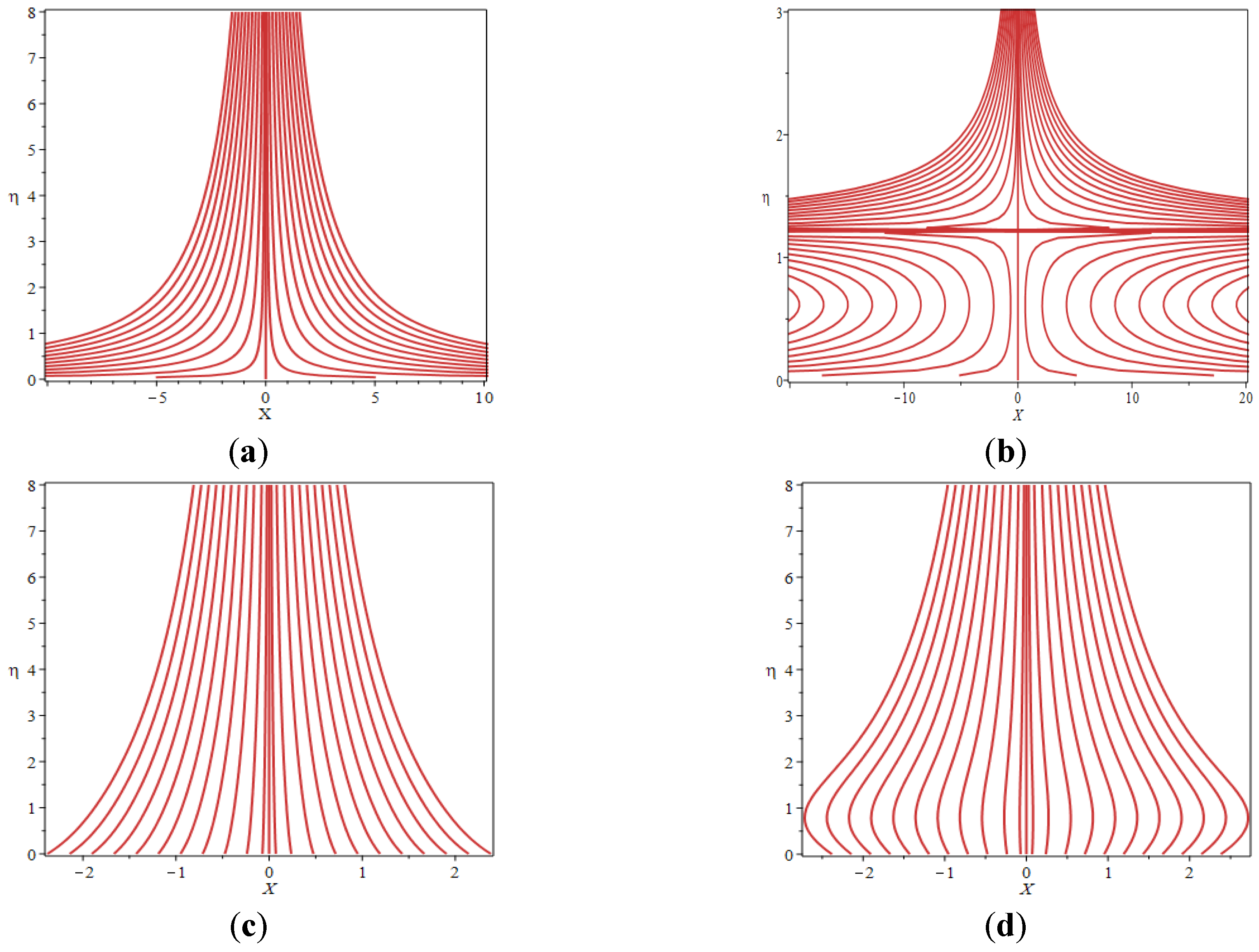
Figure 6 depicts the streamlines of the Sutterby fluid under a number of settings. In particular, Figure 6a shows the streamlines when the sheet is impermeable and stretching at the rate of 1.4, while Figure 6b illustrates the streamlines when the sheet is impermeable and shrinking. The reverse flow in Figure 6b is noticeable and proves that the shrinking sheet’s state instigates the reverse flow. Next, the streamlines for the fluid flow under the suction influence can be examined (see Figure 6c,d). The reverse flow is now absent past the permeable shrinking sheet (Figure 6d). Thus, it is proved that mass suction succeeds in sustaining the laminar boundary layer flow over a shrinking surface. Figure 6e,f shows the behavior of fluid flow when the rate of stretching or shrinking increases; the fluid pattern being pulled at the surface of the sheet is clear, and again the reverse flow is absent.
7. Conclusions
The present numerical investigation aimed to reveal the Sutterby nanofluid fluid flow and heat transfer over a permeable stretching/shrinking surface together with the effects of thermal radiation and magnetohydrodynamics (MHD). The appropriate form of the similarity transformations for the present flow problem was derived using scaling group analysis. The newly derived similarity variables then transformed the mathematical model into a more straightforward form to solve the boundary value problem utilizing the solver function bvp4c in the MATLAB software. The significant results are summarized as follows:
- An increment in the suction parameter, the Deborah number, and the nanoparticle volume fraction delay flow separation.
- The dominance of the magnetic parameter in the fluid flow regime accelerates flow separation.
- Non-unique solutions are observed when governing parameters, such as the suction parameter, the Deborah number, the magnetic number, the radiation parameter, and the nanoparticle volume fraction, vary.
- The increment in the radiation parameter slightly enhances the convective heat transfer rate past a permeable shrinking sheet.
- Stability analysis elucidates the first solution as a stable solution, and the second solution as an unstable solution.
Author Contributions
Conceptualization, M.M.F., K.N., M.F.M.B., I.H. and R.R.; methodology, M.M.F., K.N. and M.F.M.B.; software, M.M.F.; validation, M.M.F., K.N., M.F.M.B., I.H. and R.R.; formal analysis, M.M.F., K.N. and M.F.M.B.; investigation, M.M.F., K.N. and M.F.M.B.; writing—original draft preparation, M.M.F., K.N., M.F.M.B., I.H. and R.R.; writing—review and editing, M.M.F., K.N., M.F.M.B., I.H. and R.R.; funding acquisition, I.H. All authors have read and agreed to the published version of the manuscript.
Funding
This research was funded by the Ministry of Education Malaysia (Project Code: FRGS/1/2019/STG06/UKM/01/2) and the APC was funded by the Ministry of Education Malaysia (Project Code: FRGS/1/2019/STG06/UKM/01/2). The author from Universiti Teknologi Malaysia (UTM) would like to acknowledge the Ministry of Education (MOE) and Research Management Centre-UTM for supported this work under the research grant (vote number 17J52).
Conflicts of Interest
The authors declare no conflict of interest.
Nomenclature
| Roman letters | |
| dimensional positive constant | |
| A1 | first order Rivlin–Erickson tensor |
| magnetic field strength | |
| specific heat capacity | |
| CH3(CH2)4CH3 | n-Hexane |
| Deborah number | |
| material time constant | |
| Fe3O4 | magnetite |
| constant mass transfer parameter | |
| I | identity tensor |
| thermal conductivity | |
| Rosseland mean absorption coefficient | |
| magnetic parameter | |
| power-law index | |
| pressure | |
| Prandtl number | |
| radiation parameter | |
| S | extra stress tensor |
| T | Cauchy stress tensor |
| dimensional time variable | |
| wall temperature | |
| free stream temperature | |
| reference temperature | |
| dimensionless velocity | |
| dimensional velocity | |
| reference velocity | |
| V | velocity field |
| normal reference velocity | |
| dimensionless surface mass flux velocity | |
| dimensional surface mass flux velocity | |
| dimensionless Cartesian coordinates | |
| dimensional Cartesian coordinates | |
| Greek letters | |
| thermal diffusivity | |
| second invariant strain tensor | |
| smallest eigenvalue | |
| stretching/shrinking parameter | |
| critical value | |
| similarity variable | |
| dimensionless temperature | |
| viscosity at low shear rates | |
| dynamic viscosity | |
| kinematic viscosity | |
| density | |
| electrical conductivity | |
| Stefan Boltzmann constant | |
| dimensionless time variable | |
| nanoparticle volume fraction | |
| stream function | |
| Subscripts | |
| base fluid | |
| condition at the free stream | |
| nanofluid | |
| solid fractions | |
| condition at the wall | |
| Superscript | |
| differentiation with respect to | |
References
- Sutterby, J.L. Laminar converging flow of dilute polymer solutions in conical sections: Part I. Viscosity data, new viscosity model, tube flow solution. AIChE J. 1966, 12, 63–68. [Google Scholar] [CrossRef]
- Sutterby, J.L. Laminar converging flow of dilute polymer solutions in conical sections. II. Trans. Soc. Rheol. 1965, 9, 227–241. [Google Scholar] [CrossRef]
- Batra, R.L.; Eissa, M. Helical flow of a Sutterby model fluid. Polym. Plast. Technol. Eng. 1994, 33, 489–501. [Google Scholar] [CrossRef]
- Bergeron, V. Designing intelligent fluids for controlling spray applications. C. R. Phys. 2003, 4, 211–219. [Google Scholar] [CrossRef]
- Giudice, D.; Haward, S.J.; Shen, A.Q. Relaxation time of dilute polymer solutions: A microfluidic approach. J. Rheol. 2017, 61, 327–337. [Google Scholar] [CrossRef] [Green Version]
- Rehage, H.; Hoffmann, H. Viscoelastic surfactant solutions: Model systems for rheological research. Mol. Phys. 1991, 74, 933–973. [Google Scholar] [CrossRef]
- Fujii, T.; Miyatake, O.; Fujii, M.; Tanaka, H.; Murakami, K. Natural convective heat transfer from a vertical isothermal surface to a non-Newtonian Sutterby fluid. Int. J. Heat Mass Tranf. 1973, 16, 2177–2187. [Google Scholar]
- Fujii, T.; Miyatake, O.; Fujii, M.; Tanaka, H.; Murakami, K. Natural convective heat-transfer from a vertical surface of uniform heat flux to a non-Newtonian Sutterby fluid. Int. J. Heat Mass Tranf. 1974, 17, 149–154. [Google Scholar]
- Choi, S.U.S.; Eastman, J.A. Enhancing thermal conductivity of fluids with nanoparticles. ASME Publ. Fed. 1995, 231, 99–103. [Google Scholar]
- Mahian, O.; Kolsi, L.; Amani, M.; Estellé, P.; Ahmadi, G.; Kleinstreuer, C.; Marshall, J.S.; Taylor, R.A.; Abu-Nada, E.; Rashidi, S.; et al. Recent advances in modeling and simulation of nanofluid flows-Part II: Applications. Phys. Rep. 2019, 791, 1–59. [Google Scholar] [CrossRef]
- Naganthran, K.; Basir, M.F.M.; Alharbi, S.O.; Nazar, R.; Alwatban, A.M.; Tlili, I. Stagantion point flow with time-dependent bionanofluid past a sheet: Richardson extrapolation technique. Processes 2019, 7, 722. [Google Scholar] [CrossRef] [Green Version]
- Pop, I.; Naganthran, K.; Nazar, R.; Ishak, A. The effect of vertical throughflow on the boundary layer flow of a nanofluid past a stretching/shrinking sheet. Int. J. Numer. Method Heat 2017, 27, 1910–1927. [Google Scholar] [CrossRef]
- Zainal, N.A.; Nazar, R.; Naganthran, K.; Pop, I. Unsteady three-dimensional MHD non-axisymmetric Homann stagnation point flow of a hybrid nanofluid with stability analysis. Mathematics 2020, 8, 784. [Google Scholar] [CrossRef]
- Khan, M.I.; Qayyum, S.; Hayat, T.; Alsaedi, A. Stratified flow of Sutterby fluid with homogeneous-heterogeneous reactions and Catteneo-Christov heat flux. Int. J. Numer. Method Heat 2019, 29, 2977–2992. [Google Scholar] [CrossRef]
- Mir, N.A.; Alqarni, M.S.; Farooq, M.; Malik, M.Y. Analysis of heat generation/absorption in thermally stratified Sutterby fluid flow with Cattaneo-Christov theory. Microsyst. Technol. 2019, 25, 3365–3373. [Google Scholar]
- Mouli, G.B.C.; Gangadhar, K.; Raju, B.H.S. On spectral relaxation approach for Soret and Dufour effects on Sutterby fluid past a stretching sheet. Int. J. Ambient Energy 2019. [Google Scholar] [CrossRef]
- Nadeem, S.; Maraj, E.N. Peristaltic flow of Sutterby nanofluid in a curved channel with compliant walls. J. Comput. Theor. Nanos. 2015, 12, 226–233. [Google Scholar] [CrossRef]
- Akbar, N.S.; Nadeem, S. Nano Sutterby fluid model for the peristaltic flow in small intestines. J. Comput. Theor. Nanos. 2013, 10, 2491–2499. [Google Scholar] [CrossRef]
- Hayat, T.; Ayub, S.; Alsaedi, A.; Tanveer, A.; Ahmad, B. Numerical simulation for peristaltic activity of Sutterby fluid with modified Darcy’s law. Results Phys. 2017, 7, 762–768. [Google Scholar] [CrossRef]
- Ahmad, S.; Farooq, M.; Javed, M.; Anjum, A. Double stratification effects on chemically reactive squeezed Sutterby fluid flow with thermal radiation and mixed convection. Results Phys. 2018, 8, 1250–1259. [Google Scholar] [CrossRef]
- Hayat, T.; Afzal, S.; Khan, M.I.; Alsaedi, A. Irreversibility aspects to flow of Sutterby fluid subject to nonlinear heat flux and Joule heating. Appl. Nanosci. 2019, 9, 1215–1226. [Google Scholar] [CrossRef]
- Hayat, T.; Masood, F.; Qayyum, S.; Alsaedi, A. Sutterby fluid flow subject to homogeneous-heterogeneous reactions and nonlinear radiation. Physica A 2020, 544, 123439. [Google Scholar] [CrossRef]
- Nawaz, M. Role of hybrid nanoparticles in thermal performance of Sutterby fluid, the ethylene glycol. Physica A 2020, 537, 122447. [Google Scholar] [CrossRef]
- Wang, F.; Wang, N.; Yu, F.; Wang, X.; Cui, J. Study on micro-structure, solid solubility and tensile properties of 5A90 Al-Li alloy cast by low-frequency electromagnetic casting processing. J. Alloys Compd. 2020, 820, 153318. [Google Scholar] [CrossRef]
- Beg, O.A.; Ferdows, M.; Karim, M.E.; Hasan, M.M.; Bég, T.A.; Shamshuddin, M.D.; Kadir, A. Computation of non-isothermal thermo-convective micropolar fluid dynamics in a wall MHD generator system with non-linear distending wall. Int. J. Appl. Comput. Math. 2020, 6, 42. [Google Scholar]
- Raptis, A.; Perdikis, C.; Takhar, H.S. Effect of thermal radiation on MHD flow. Appl. Math. Comput. 2004, 153, 645–649. [Google Scholar] [CrossRef]
- Sabir, Z.; Imran, A.; Umar, M.; Zeb, M.; Shoaib, M.; Raja, M.A.Z. A numerical approach for two-dimensional Sutterby fluid flow bounded at a stagnation point with an inclined magnetic field and thermal radiation impacts. Therm. Sci. 2020, 186. [Google Scholar] [CrossRef]
- Bilal, S.; Sohail, M.; Naz, R.; Malik, M.Y.; Alghamdi, M. Upshot of ohmically dissipated Darcy-Forchheimer slip flow of magnetohydrodynamic Sutterby fluid over radiating linearly stretched surface in view of Cash and Crap method. Appl. Math. Mech. Engl. Ed. 2019, 40, 861–876. [Google Scholar] [CrossRef]
- Prandtl, L. Über Flussigkeitsbewegungen bei sehr kleiner Reibung. Verhandl. III Intern. Math. 1904, 484–491. Available online: https://ci.nii.ac.jp/naid/20000989592/ (accessed on 20 July 2020).
- Schwarz, F. Symmetries of differential equations: From Sophus Lie to computer algebra. SIAM Rev. 1988, 30, 450–481. [Google Scholar] [CrossRef]
- Pakdemirli, M.; Yurusoy, M. Similarity transformations for partial differential equations. SIAM Rev. 1998, 40, 96–101. [Google Scholar] [CrossRef]
- Naganthran, K.; Basir, M.F.M.; Thumma, T.; Ige, E.O.; Nazar, R.; Tlili, I. Scaling group analysis of bioconvective micropolar fluid flow and heat transfer in a porous medium. J. Therm. Anal. Calorim. 2020. [Google Scholar] [CrossRef]
- Hamad, M.A.A.; Pop, I. Scaling transformations for boundary layer flow near the stagnation-point on a heated permeable stretching surface in a porous medium saturated with a nanofluid and heat generation/absorption effects. Transp. Porous Media 2011, 87, 25–39. [Google Scholar] [CrossRef]
- Azhar, E.; Iqbal, Z.; Maraj, E.N. Impact of entropy generation on stagnation-point flow of Sutterby nanofluid: A numerical analysis. Z. Naturforsch. 2016, 71, 837–848. [Google Scholar] [CrossRef]
- Azhar, E.; Iqbal, Z.; Ijaz, S.; Maraj, E.N. Numerical approach for stagnation point flow of Sutterby fluid impinging to Cattaneo-Christov heat flux model. Pramana J. Phys. 2018, 91, 61. [Google Scholar] [CrossRef]
- Naganthran, K.; Basir, M.F.M.; Kasihmuddin, M.S.M.; Ahmed, S.E.; Olumide, F.B.; Nazar, R. Exploration of dilatant nanofluid effects conveying microorganism utilizing scaling group analysis: FDM Blottner. Physica A 2020, 549, 124040. [Google Scholar] [CrossRef]
- Brinkman, H. The viscosity of concentrated suspensions and solutions. J. Chem. Phys. 1952, 20, 571. [Google Scholar] [CrossRef]
- Hewitt, G.F.; Shires, G.L.; Bott, T.R. Process Heat Transfer; CRC Press: Boca Raton, FL, USA, 1994; p. 987. [Google Scholar]
- Merkin, J.H. Mixed convection boundary layer flow on a vertical surface in a saturated porous medium. J. Eng. Math. 1980, 14, 301–313. [Google Scholar] [CrossRef]
- Merkin, J.H. On dual solutions occurring in mixed convection in a porous medium. J. Eng. Math. 1985, 20, 171–179. [Google Scholar] [CrossRef]
- Bhattacharyya, K.; Layek, G.C. Effects of suction/blowing on steady boundary layer stagnation-point flow and heat transfer towards a shrinking sheet with thermal radiation. Int. J. Heat Mass Tranf. 2011, 54, 302–307. [Google Scholar] [CrossRef]
- Tie-Gang, F.; Ji, Z.; Shan-Shan, Y. Viscous flow over an unsteady shrinking sheet with mass transfer. Chin. Phys. Lett. 2009, 26, 014703. [Google Scholar] [CrossRef]
Figure 1.
Schematic diagram of the present problem: (a) shrinking sheet ; (b) stretching sheet
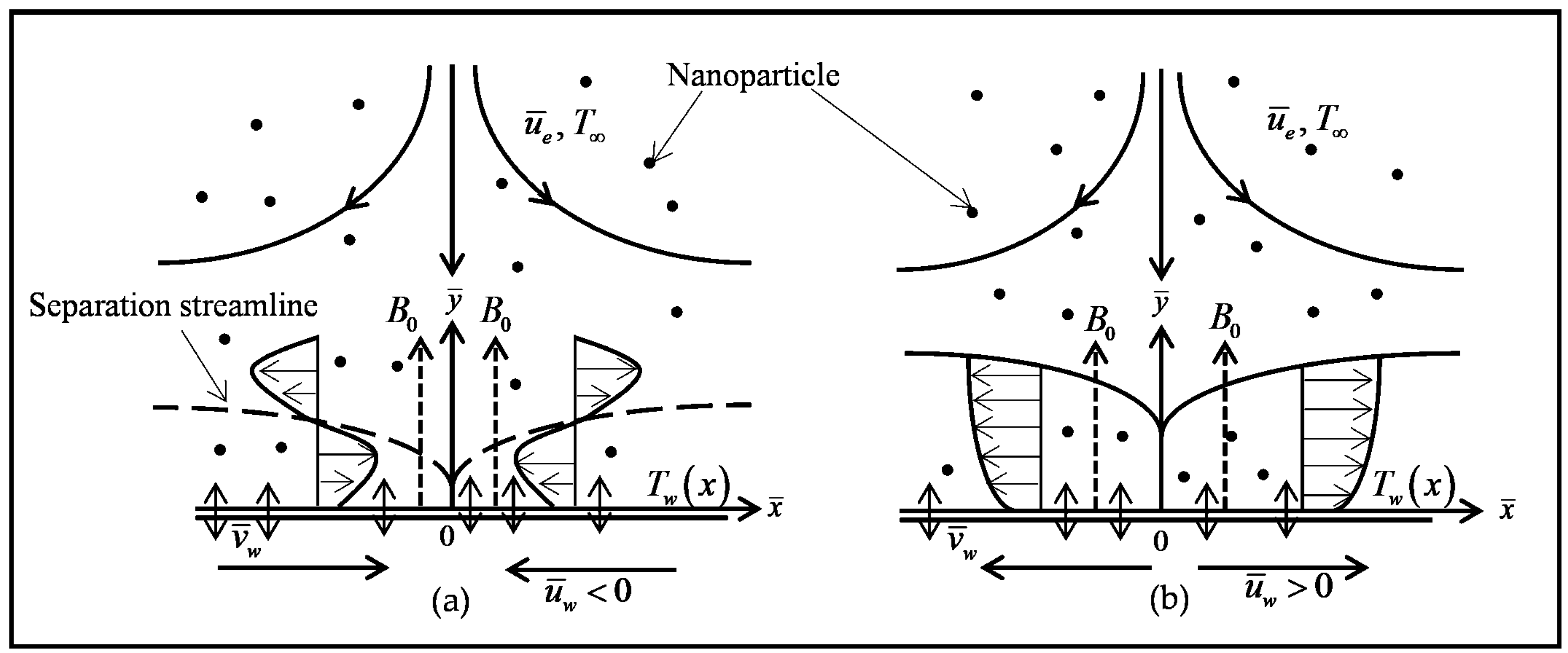
Figure 2.
Impact of the suction parameter (s) on: (a) the reduced skin friction coefficient; (b) velocity profiles as s varies when , and
Figure 2.
Impact of the suction parameter (s) on: (a) the reduced skin friction coefficient; (b) velocity profiles as s varies when , and
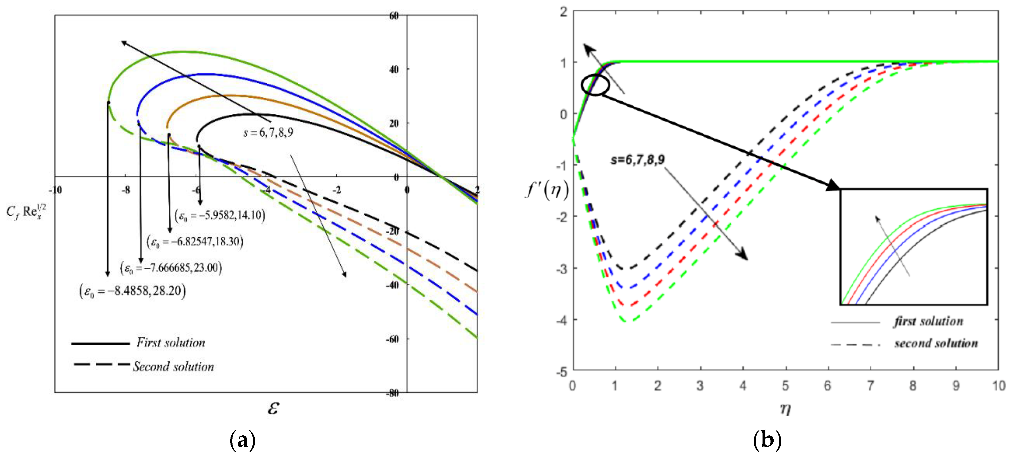
Figure 3.
Impact of the Deborah number (De) on: (a) the reduced skin friction coefficient; (b) velocity profiles as De varies when , and .
Figure 3.
Impact of the Deborah number (De) on: (a) the reduced skin friction coefficient; (b) velocity profiles as De varies when , and .
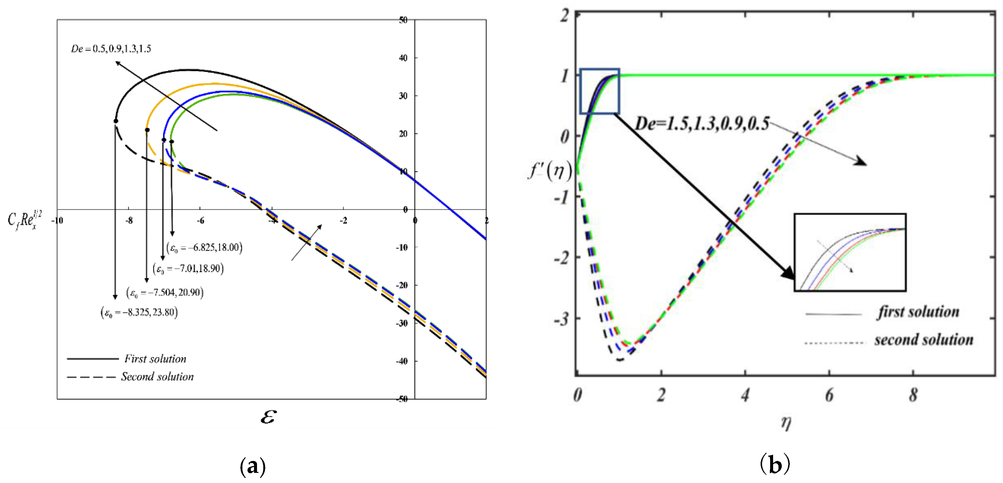
Figure 4.
Impact of the magnetic parameter (M) on: (a) the reduced skin friction coefficient; (b) velocity profiles as M varies past a shrinking sheet ; (c) velocity profiles as M varies past a stretching sheet when , and .
Figure 4.
Impact of the magnetic parameter (M) on: (a) the reduced skin friction coefficient; (b) velocity profiles as M varies past a shrinking sheet ; (c) velocity profiles as M varies past a stretching sheet when , and .
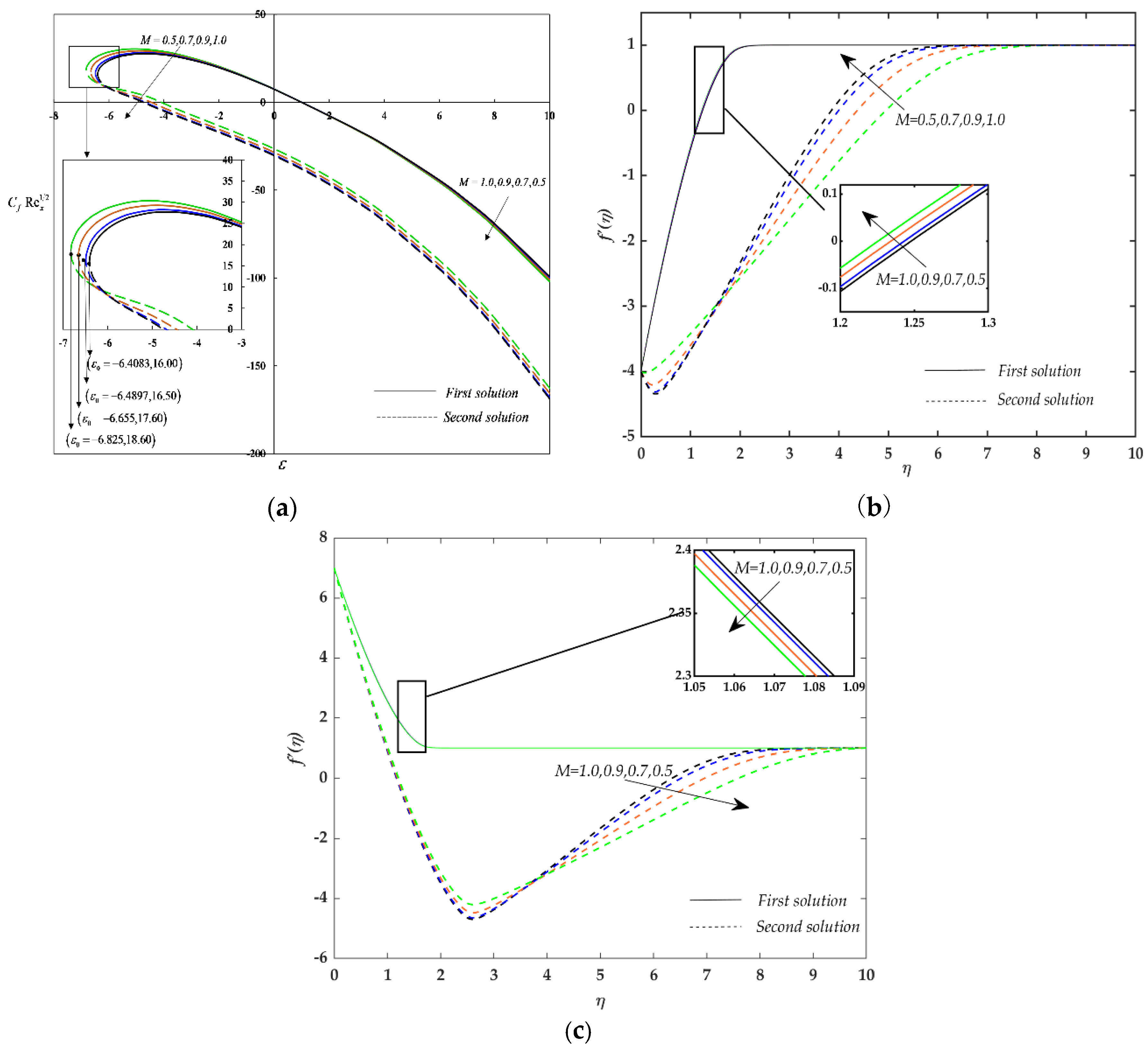
Figure 5.
Impact of the nanoparticle volume fraction () on: (a) the reduced skin friction coefficient; (b) velocity profiles as varies when , and ϕ = 0.02.
Figure 5.
Impact of the nanoparticle volume fraction () on: (a) the reduced skin friction coefficient; (b) velocity profiles as varies when , and ϕ = 0.02.
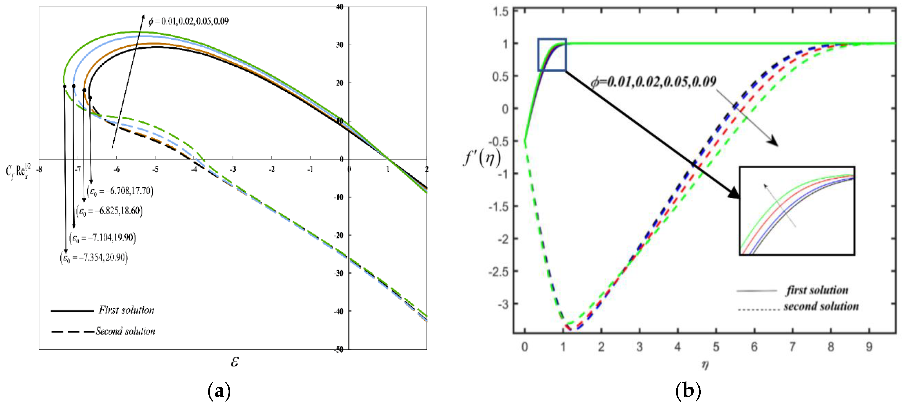
Figure 6.
Streamlines when (a) (b) (c) (d) (e) (f) .


Table 1.
The thermo physical characteristics of the essential fluid and nanoparticles.
| Physical Properties | Fluid Phase (n-Hexane /CH3(CH2)4CH3) | Solid Phase Magnetite (Fe3O4) |
|---|---|---|
| 2.78 | 670 | |
| 551 | 5180 | |
| 82 | 9.7 | |
| Pr | 4.36 |
Table 2.
Numerical validation of when in [41].
Table 2.
Numerical validation of when in [41].
| Present Result | Bhattacharyya et al. [41] | |||
|---|---|---|---|---|
| First Solution | Second Solution | First Solution | Second Solution | |
| 1.40224078 | ||||
| 1.49566974 | ||||
| 1.50715589 | ||||
| 1.48929822 | ||||
| 1.32881685 | 0 | |||
| 1.08223113 | 0.11670214 | |||
*c/a is the stretching/shrinking parameter in [41].
Table 3.
The effect of the radiation parameter (Rd) on the reduced local Nusselt number when , and as varies.
Table 3.
The effect of the radiation parameter (Rd) on the reduced local Nusselt number when , and as varies.
| Radiation Parameter (Rd) | ||||||
|---|---|---|---|---|---|---|
| First Solution | Second Solution | |||||
| −1.5 | 0.5 | −1846.311663 | −1846.31001 | |||
| −3.5 | −1845.804534 | −1845.803095 | ||||
| −5.5 | −1845.296838 | −1845.296378 | ||||
| −6.5 | −1845.042742 | −1845.042486 | ||||
| −1.5 | 1.2 | −1846.051576 | −1846.046864 | |||
| −3.5 | −1845.195172 | −1845.191067 | ||||
| −5.5 | −1844.337149 | −1844.335834 | ||||
| −6.5 | −1843.907426 | −1843.906694 | ||||
| −1.5 | 3.5 | −1845.128211 | −1845.099751 | |||
| −3.5 | −1844.064298 | −1844.051593 | ||||
| −5.5 | −1842.553219 | −1842.549137 | ||||
| −6.5 | −1841.795465 | −1841.793188 | ||||
Table 4.
Lowest eigenvalues when , and as varies.
| ε | γ1 | |
|---|---|---|
| First Solution | Second Solution | |
| −6.8 | 0.5844 | −0.4163 |
| −6.82 | 0.2842 | −0.1794 |
| −6.822 | 0.2339 | −0.1354 |
| −6.8250 | 0.1128 | −0.0237 |
| −6.82520 | 0.0961 | −0.0077 |
| −6.825250 | 0.0911 | −0.0028 |
© 2020 by the authors. Licensee MDPI, Basel, Switzerland. This article is an open access article distributed under the terms and conditions of the Creative Commons Attribution (CC BY) license (http://creativecommons.org/licenses/by/4.0/).
Share and Cite
MDPI and ACS Style
Fayyadh, M.M.; Naganthran, K.; Basir, M.F.M.; Hashim, I.; Roslan, R. Radiative MHD Sutterby Nanofluid Flow Past a Moving Sheet: Scaling Group Analysis. Mathematics 2020, 8, 1430. https://doi.org/10.3390/math8091430
AMA Style
Fayyadh MM, Naganthran K, Basir MFM, Hashim I, Roslan R. Radiative MHD Sutterby Nanofluid Flow Past a Moving Sheet: Scaling Group Analysis. Mathematics. 2020; 8(9):1430. https://doi.org/10.3390/math8091430
Chicago/Turabian StyleFayyadh, Mohammed M., Kohilavani Naganthran, Md Faisal Md Basir, Ishak Hashim, and Rozaini Roslan. 2020. "Radiative MHD Sutterby Nanofluid Flow Past a Moving Sheet: Scaling Group Analysis" Mathematics 8, no. 9: 1430. https://doi.org/10.3390/math8091430
Note that from the first issue of 2016, this journal uses article numbers instead of page numbers. See further details here.