
Dynamic Characteristics Analysis of ISD Suspension System under Different Working Conditions


1
School of Mechanical Engineering and Automation, Northeastern University, Shenyang 110819, China
2
State Key Laboratory of Automotive Simulation and Control, Jilin University, Changchun 130025, China
*
Author to whom correspondence should be addressed.
Mathematics 2021, 9(12), 1345; https://doi.org/10.3390/math9121345
Submission received: 26 May 2021
/
Revised: 7 June 2021
/
Accepted: 8 June 2021
/
Published: 10 June 2021
(This article belongs to the Special Issue Dynamical Systems and System Analysis)
Abstract
:The “inerter-spring-damper” (ISD) suspension system is a suspension system composed of an inerter, spring, and damper. To study the ride comfort and stability of the vehicle by using the ISD suspension system, a vehicle model with ISD suspension is established in this paper. The vehicle model including vertical, pitch, roll, and yaw motion of the vehicle body. Based on the vehicle model, the differential equation of motion with ISD suspension is obtained. The dynamic responses of the ISD suspension system are investigated by using different road excitations. At the same time, the influence of coupled excitation and single excitation on the vibration reduction performance of the ISD suspension system is studied. Then, the dynamic responses of ISD suspension and passive suspension are compared, and the improvement of comprehensive vibration reduction performance of ISD suspension system is quantitatively analyzed. The numerical results illustrate the ISD suspension has the optimal vehicle speed under different road excitations, and the comprehensive vibration reduction performance of the ISD suspension is the best when driving at the optimal vehicle speed. Under different types of road excitation, ISD suspension shows excellent comprehensive vibration reduction performance. ISD suspension is more suitable for vibration reduction of complex roads than that of a single road.
1. Introduction
The suspension is an important part of the vehicle, which is responsible for connecting the body and wheels. Suspension not only plays a supporting role in the vehicle but also can be used to mitigate the impact caused by road roughness and restrain the vibration of the vehicle body. Improvement of suspension vibration reduction performance has been a hot issue in the vehicle engineering field. The passive suspension is composed of spring and damper [1,2]. It has a simple structure and high reliability. However, passive suspension cannot coordinate the contradiction between vehicle ride comfort and stability, which limits the further improvement of passive suspension vibration reduction performance. Based on the existing problems of vehicle passive suspension, scholars have carried out a lot of research on active suspension [3,4] and semi-active suspension [5,6]. To improve vehicle stability, a slow active suspension was proposed [7], and the effectiveness of the control strategy was verified by simulation. To reduce the risk of a vehicle rollover, the control system of active suspension was studied [8]. However, active and semi-active suspensions need energy input, which requires a high accuracy and high cost of the control system.
In 2002, the concept of inerter was first proposed [9]. The invention of inerter provides a new possibility for improving the performance of the vehicle suspension system [10]. A one quarter vehicle model with ISD suspension was established and studied the influence of different parameters on ride comfort [11]. The performance of the gear rack inerter and ball screw inerter was tested, the results showed that the performance of the inerter was greatly affected by friction factors in a low-frequency band [12]. A classification process for finding effective branches of a mechanical network was described, and a design method for a passive mechanical network of ISD suspension was proposed [13,14]. Electromechanical similarity theory and mechanical network synthesis theory were used to determine the structure of ISD suspension. The feasibility of this method was proved by a bench test [15]. Inerter was applied to train suspension vibration reduction, which improved the vibration reduction performance of the train [16,17]. An ISD damper mechanism was applied to building vibration isolation to improve the isolation performance of buildings [18]. An ISD suspension structure based on the principle of dynamic vibration absorption was proposed, and the performance improvement was verified by a single-wheel bench test [19]. The damper was replaced by an ISD topology based on traditional passive suspension and studied the influence of different ISD topology on the vibration reduction performance [20]. The literature [21,22,23,24,25,26] studied the effect of the ISD module composed of inerter, spring, and damper on the vibration reduction performance of the system. The literature [27,28,29] studied the influence of the control system on the damping performance of the damping system with inertial damping elements. Ma [30] developed an inerter-based vibration isolation system for heave motion mitigation of semi-submersible platforms subjected to sea waves. Liu [31] investigated the potential for reduction in road damage by incorporating the inerter element into truck suspension systems. Shen [32] provided an approach for the optimal design of both the mechanical and the electrical parts for an inerter-based mechatronic device in vehicle suspension. However, the dynamic characteristics of the ISD suspension system under various types of road excitation still have room for further exploration.
The main contributions of this paper include the establishment of a whole vehicle dynamic model with ISD suspension and the analysis of vehicle dynamic response under different types of road excitation. Considering the vertical, pitch, roll, and yaw motion of the vehicle body, the vehicle model contains more abundant motion relations, more in line with the actual running state of the vehicle, and more able to reflect the changing law of ISD suspension performance.
The arrangement of this paper is as follows. In Section 2, considering the vertical, pitching, roll, and yaw motion of the body, the vehicle model and the dynamic equation of the vehicle system are established, and the dynamic equation is solved simultaneously. In Section 3, three representative road excitation models are introduced, which are fitting periodic road excitation model, consecutive speed control humps model, and coupled road excitation model. In Section 4, the optimal speed of ISD suspension under different road excitation is obtained. At the same time, the dynamic characteristics of the ISD suspension system under different working conditions are analyzed. Taking the passive suspension as a comparative object, the improvement degree of ride comfort and stability of the vehicle with ISD suspension is explored through the performance evaluation indexes such as centroid acceleration, pitch angular acceleration, roll angular acceleration, yaw angular acceleration, suspension working space and tyre dynamic load. At the end of the paper, some conclusions of the research are drawn in Section 5.
2. Dynamic Model of Vehicle Suspension System
2.1. Vehicle Model with ISD Suspension
The inerter breaks through the limitation of single terminal grounding of the mass block. It is a kind of double terminal vibration damping element. The physical realization structure of the inerter mainly includes ball screw inerter, rack and pinion inerter, and hydraulic inerter. Compared with other forms of inerter, the ball screw inerter has the advantages of simple structure and easy installation.
The ball screw inerter is shown in Figure 1.
In Figure 1, 1–4 represent motion states respectively. State 1 represents the initial position of the inerter, State 2 represents the position when the inerter moves downward, State 3 represents the position when the inerter moves downward to the lowest point, and State 4 represents the position when the inerter moves upward. When the two ends of the ball screw inerter are stressed, the two ends of the inerter will produce relative motion along the axis direction, and the ball screw pair will convert the linear motion into the rotating motion of the screw, and then make the flywheel rotate. The force on both ends of the inerter is finally converted into the driving torque of the screw and flywheel rotation, and then the vibration signal is attenuated. Then, the force acting on both ends of the ball screw inerter can be written as:
where m0 is the mass of the flywheel, r is the radius of the flywheel, p is the lead of the ball screw pair, s is the relative velocity of the two ends of the inerter, b is the inertance of the inerter.
The ISD damping module is shown in Figure 2.
In Figure 2, the ISD damping module is composed of the first stage suspension and the second stage suspension in series. In the first stage, k1 is the spring stiffness, c1 is the damping coefficient. In the second stage, k2 is the spring stiffness, b is the inertance, c2 is the damping coefficient.
To explore the improvement of ISD suspension with inerter on ride comfort, rollover prevention ability, and lateral stability, a vehicle model with ISD suspension is established. The vehicle model with ISD suspension is shown in Figure 3.
The parameters of the vehicle model come from a mature passenger car, and the detailed parameters are shown in Table 1.
In Figure 3, the origin O of the coordinate system is located at the center of mass of the spring load mass. The same direction as the vehicle’s forward direction is the x-axis. In the horizontal plane of the origin O, the y-axis is perpendicular to the x-axis, the y-axis is positive in the left direction of the vehicle, and the z-axis is positive in the vertical direction of the O-point. In Figure 3, ms is the vehicle body mass, ω is the vehicle yaw rate, φ is the roll angle of the vehicle body, θ is the pitch angle of the vehicle body, ki1 (i = 1, 2, 3, 4) is the spring stiffness of the first stage suspension, ci1 (i = 1, 2, 3, 4) is the damping coefficient of the first stage suspension, ki2 (i = 1, 2, 3, 4) is the spring stiffness of the second stage suspension, ci2 (i = 1, 2, 3, 4) is the damping coefficient of the second stage suspension, bi (i = 1, 2, 3, 4) is the inertance of the suspension, zsi (i = 1, 2, 3, 4) is the vertical displacement of spring-loaded mass at the front and rear wheels, zri (i = 1, 2, 3, 4) is the vertical displacement of common end between suspension stages, zui (i = 1, 2, 3, 4) is the vertical displacement of front and rear non-spring loaded mass, ki3 (i = 1, 2, 3, 4) is the tyre stiffness, and zgi (i = 1, 2, 3, 4) is the vertical displacement of front and rear non-spring loaded mass.
2.2. Dynamic Model of Vehicle System
To analyze the dynamic characteristics of the vehicle model with ISD suspension, the dynamic model of the vehicle system is established, and the differential equation of motion is shown below.
Vehicle longitudinal balance equation can be rewritten as:
where m is the vehicle mass, ms is the vehicle body mass, v is the longitudinal velocity, u is the lateral velocity, ω is the vehicle yaw rate, H is the height from the vehicle centroid to the roll center, φ is the roll angle of the vehicle body, and θ is the pitch angle of the vehicle body.
Vehicle lateral balance equation can be rewritten as:
The equilibrium equation of vertical direction for spring-loaded mass can be rewritten as:
where zs is the vertical displacement of the vehicle body, Ls is the distance from the centroid of vehicle mass to body mass.
The equilibrium equation of roll motion of spring-loaded mass can be rewritten as:
where Ix is the body roll moment of inertia, Iy is the body pitch moment of inertia, Iz is the body yaw moment of inertia, Ixz is the inertia product of body mass.
The equilibrium equation of pitch motion of spring-loaded mass can be rewritten as:
Vehicle yaw motion balance equation can be rewritten as:
where I is the vehicle yaw moment of inertia.
Summation of vertical outward forces on spring-loaded mass can be rewritten as:
where Fi (i = 1, 2, 3, 4) is the force of the suspension system.
According to the equal force of the first and second suspensions, the forces can be written as follows:
where ki1 (i = 1, 2, 3, 4) is the spring stiffness of the first stage suspension, ci1 (i = 1, 2, 3, 4) is the damping coefficient of the first stage suspension, ki2 (i = 1, 2, 3, 4) is the spring stiffness of the second stage suspension, ci2 (i = 1, 2, 3, 4) is the damping coefficient of the second stage suspension, bi (i = 1, 2, 3, 4) is the inertance of the suspension, zsi (i = 1, 2, 3, 4) is the vertical displacement of spring-loaded mass at the front and rear wheels, zri (i = 1, 2, 3, 4) is the vertical displacement of common end between suspension stages, zui (i = 1, 2, 3, 4) is the vertical displacement of front and rear non-spring loaded mass.
The vertical motion equation of non-spring-loaded mass can be rewritten as:
where ki3 (i = 1, 2, 3, 4) is the tyre stiffness, mui (i = 1, 2, 3, 4) is the front and rear non-spring-loaded mass, zgi (i = 1, 2, 3, 4) is the vertical displacement of front and rear non-spring loaded mass.
When the pitch angle and roll angle are small, the approximation can be rewritten as:
where a is the distance from the front axle to the centroid, e is the distance from the rear axle to the centroid, d is the half tread of left and right wheels.
The sum of the roll-out moments of spring-loaded mass can be rewritten as:
The sum of pitching external moments of spring-loaded mass can be rewritten as:
Vector representations of vehicle motion state variables can be rewritten as:
The derivative of Equation (14) can be rewritten as:
The coefficient matrix of differential equations can be rewritten as:
where,
The equivalent matrix of a system of differential equations can be rewritten as:
where,
The above differential equations of motion are separated by the operation of matrices and vectors, which can be rewritten as:
Submitting the Equations (15), (16) and (18) into Equation (20), the system equation of state can be rewritten as:
3. Different Types of Road Incentive Models
Road roughness generally refers to the difference between the actual road surface and the ideal level. In the course of driving, the main incentive is the input of the degree of road roughness. There are two main forms of road roughness: one is the common uneven road surface caused by the construction level of workers, the other is the special uneven road surface formed by the speed control humps.
3.1. Fitting Periodic Road Excitation Model
In previous studies, when a vehicle passes through an ordinary uneven road surface, the road surface excitation is expressed as a single periodic excitation. However, in the actual driving process of vehicles, the types of the road surface are various, and the road excitation is often formed by a variety of signal fitting. Therefore, this paper establishes a fitting periodic road excitation model. The fitting periodic road excitation model is established as shown in Figure 4.
In Figure 4, compared with the single periodic excitation model in the prior work [33,34], the fitting periodic road excitation model adopted in this paper is composed of signals of different frequencies, and the influence of vehicle speed on the excitation is considered. At different speeds, the time difference between the front and rear wheels is different. Therefore, the fitting periodic road excitation model is more consistent with the road conditions of vehicles.
The input displacement of the front wheel of the vehicle can be rewritten as:
where A1 is the amplitude of the first signal, and is set as 0.03 m. ω1 is the angular frequency of the first signal, and is set as 7.9 Hz. A2 is the amplitude of the second signal, and is set as 0.03 m. ω2 is the angular frequency of the second signal, and is set as () Hz.
The input displacement of the rear wheel of the vehicle can be rewritten as:
where,
3.2. Consecutive Speed Control Humps Model
Because of the short distance of the single speed control humps, the time when the vehicle passes through the excitation is very short, so the influence time on the vehicle is also very short. However, the distance between the consecutive speed control humps and the single-speed control humps is relatively long, so it will cause more complex dynamics of the vehicle. Therefore, this paper establishes a road incentive model of consecutive speed control humps. The consecutive speed control humps model was established as shown in Figure 5.
In Figure 5, A is the amplitude of consecutive speed control humps, and is set as 0.015 m. v is the vehicle speed. L is the spacing between two sets of consecutive speed control humps, and is set as 6 m.
The input displacement of the front wheel of the vehicle can be rewritten as:
The input displacement of the rear wheel of the vehicle can be rewritten as:
where l1 is the width of the single-speed control hump, and is set as 0.5 m. l2 is the width between two-speed control humps, and is set as 0.5 m. N is the natural number. T1 is the time when a vehicle passes through a set of speed control humps, T2 is the time when a vehicle passes through the road between two sets of speed control humps.
3.3. Coupled Road Excitation Model
To make the road excitation closer to reality than the single harmonic excitation, the research results have a higher reference value. This paper also establishes the road excitation model when the consecutive speed control humps are coupled with the uneven road surface. Coupled road excitation is the coupling of fitting periodic road excitation and consecutive speed control humps. Its expression is as follows:
where,
The input displacement of the front wheel of the vehicle can be rewritten as:
The input displacement of the rear wheel of the vehicle can be rewritten as:
4. Dynamic Characteristics Analysis
Based on the vehicle model with the ISD suspension system established in this paper, the performance evaluation indexes of the ISD suspension system are centroid acceleration, pitch angular acceleration, roll angular acceleration, yaw angular acceleration, suspension working space, and tyre dynamic load. Under fitting periodic road excitation, consecutive speed control humps, and coupled road excitation, the ISD suspension system is analyzed in different vehicle speeds. The optimal speed of vehicle passing through different types of uneven roads can be obtained by comprehensive vibration reduction performance.
At the same time, the vibration reduction performance of ISD suspension and traditional passive suspension is compared and analyzed under this speed, and the performance improvement of ISD suspension under various types of road excitation is studied. To better understand the dynamic responses of the system intuitively, the detailed simulation condition schematic is shown in Figure 6.
To analyze the comprehensive vibration reduction performance of vehicle ISD suspension system when the vehicle passes through different types of the uneven road at different speeds, and to obtain the optimal vehicle speed when passing through different types of road, it is necessary to establish the objective function. Based on the three indexes of vehicle ride comfort, the centroid acceleration root mean square (JSD), suspension working space root mean square (DXC), and tyre dynamic load root mean square (DZH) are dimensionless, and then weighted linearly. Finally, the sum of them is obtained and the multi-objective optimization function J is established. The specific expression can be rewritten as:
where n1 is the weighted coefficient of JSD, and is set as 0.4. n2 is the weighted coefficient of DXC, and is set as 0.3. n3 is the weighted coefficient of DZH, and is set as 0.3. min (JSD) is the minimum value of JSD in variable velocity range, min (DXC) is the minimum value of DXC in variable velocity range, min (DZH) is the minimum value of DZH in variable velocity range.
4.1. Dynamic Responses under Fitting Periodic Road Excitation
Taking the vehicle model established in this paper as the simulation object, the objective function values corresponding to different vehicle speeds are analyzed under the fitting periodic road excitation, and the optimal vehicle speed is obtained when the vehicle passes through the fitting periodic road excitation. The objective function value under fitting periodic road excitation is shown in Figure 7.
In Figure 7, when the vehicle speed varies from 30 km/h to 100 km/h, with the increase of vehicle speed, the objective function value J decreases first and then increases. At the vehicle speed of 65 km/h, the objective function J is the smallest, that is to say, the optimal vehicle speed is 65 km/h, when the vehicle passes through fitting periodic road excitation at this speed, the comprehensive vibration reduction performance of ISD suspension is the best. The result shows that the vehicle speed of 65 km/h is selected to analyze the performance improvement of ISD suspension compared with passive suspension.
To demonstrate the dynamic responses of the vehicle system, the dynamic characteristics under fitting periodic road excitation are shown in Figure 8.
To quantitatively describe the performance changes, comparison of performance indicators under fitting periodic road excitation is shown in Table 2.
In Figure 8, compared with the passive suspension, the vibration reduction performance of the vehicle using ISD suspension has been effectively improved. It shows that ISD suspension with inerter can improve ride comfort and pitch, roll, and yaw stability of the vehicle. At the same time, with the continuous action of fitting periodic road excitation, the yaw angular acceleration and tyre dynamic load of passive suspension tend to increase. In the period of 0–8 s, the damping performance of passive suspension is relatively stable; in the period of 8–10 s, the damping performance of passive suspension tends to deteriorate. However, the ISD suspension has no deteriorating trend in 0–10 s, so the ISD suspension has good dynamic vibration reduction performance.
Table 2 further shows the detailed indexes of Figure 8. It is noted that the RMS values of centroid acceleration, pitch angular acceleration, roll angular acceleration, yaw angular acceleration, suspension working space, and tyre dynamic load were reduced by 70.0%, 25.2%, 5.5%, 45.2%, 80.6%, and 45.2%. The peak values were reduced by 53.1%, 24.9%, 0.3%, 65.1%, 69.5% and 66.1%, respectively. The improvement degree of centroid acceleration, yaw angular acceleration, suspension working space, and tyre dynamic load index are all more than 45%. It shows that ISD suspension has a good effect on restraining vehicle vibration and is more suitable for the practical vehicle body.
4.2. Dynamic Responses of Consecutive Speed Control Humps
As a vehicle speed control device, consecutive speed control humps play an important role in improving traffic safety. The dynamic characteristics of the vehicle system are different when the vehicle passes through the consecutive speed control humps at different speeds. Firstly, the comprehensive performance of ISD suspension when the vehicle passes through consecutive speed control humps at different speeds is explored, and the optimal speed is obtained. Then, the performance indexes of ISD suspension and passive suspension are calculated, and the performance improvement of ISD suspension is analyzed by comparing ISD suspension with passive suspension. The objective function value under consecutive speed control humps is shown in Figure 9.
In Figure 9, when the vehicle speed v is in the range of 30 km/h to 65 km/h, with the increase of vehicle speed, the objective function J decreases gradually, that is, the comprehensive performance of ISD suspension becomes better gradually. When the vehicle speed varies from 65 km/h to 80 km/h, the objective function value J fluctuates around the fixed value in the interval, and its fluctuation range is small. Overall, in the range of 65 km/h to 80 km/h, the objective function J is relatively small, that is, ISD suspension has the better comprehensive performance. When the vehicle speed v is between 80 km/h and 100 km/h, the objective function J increases with the increase of vehicle speed, and the comprehensive performance of ISD suspension decreases gradually. Therefore, the optimal speed is 80 km/h. When passing through the consecutive speed control humps, the speed can be limited to the vicinity of 65 km/h to 80 km/h.
The consecutive speed control humps can limit the speed of the vehicle and improve the safety of the vehicle. However, if the speed of the vehicle is not within the appropriate range, the consecutive speed control humps will not only not play the role of speed limit, but also affect the safety of the vehicle and passenger comfort. Therefore, when the speed of 65–80 km/h is used to drive through the consecutive speed control humps, the speed limit effect of the consecutive speed control humps is the best, and the improvement of the vibration reduction performance of ISD suspension is more obvious.
To demonstrate the dynamic responses of the vehicle system, dynamic characteristics under consecutive speed control humps are shown in Figure 10.
In Figure 10, in the period of 0–1 s, the vehicle is in the initial stage, and the performance evaluation indexes have not yet reached the steady state. However, in the period of 1–10 s, the vibration reduction performance of the vehicle with ISD suspension under the consecutive speed control humps has been effectively improved. Among them, the increase of pitch angular acceleration, yaw angular acceleration, suspension working space, and tyre dynamic load is more obvious, which shows that the ISD suspension has a better effect on restraining the vehicle body motion.
Comparison of performance indicators under consecutive speed control humps is shown in Table 3.
Table 3 further shows the detailed indexes of Figure 10. It is noted that the RMS values of centroid acceleration, roll angular acceleration, and suspension working space are reduced by 13.3%, 15.8%, 7.7%, and peak values are reduced by 6.9%, 20.3%, and 26.6%, respectively. It shows that ISD suspension has a certain effect on restraining the vertical, roll motion, and suspension travel. The RMS values of pitch angular acceleration, yaw angular acceleration, and tyre dynamic load are reduced by 33.2%, 43.7%, and 24.2%, and the peak values are reduced by 36.8%, 44.9%, and 20.7%, respectively. Compared with other indicators, the improvement effect of pitch angular acceleration, yaw angular acceleration, and tyre dynamic load is more obvious, which shows that ISD suspension can improve vehicle driving stability better.
4.3. Dynamic Responses of Coupled Road Excitation
Coupled road excitation is more in line with the actual driving road surface. Taking coupled road excitation as road input, the comprehensive vibration reduction performance of the ISD suspension system is explored when different vehicle speeds pass through coupled road excitation, and the optimal vehicle speed is obtained. At the same time, it is compared with single working condition. Besides, the ISD suspension is compared with the passive suspension under the optimal vehicle speed, and the performance improvement of ISD suspension is analyzed. The objective function value under coupled road excitation is shown in Figure 11.
In Figure 11, when the speed v is in the range of 30 km/h to 70 km/h, with the increase of speed, the objective function value J decreases gradually, that is, the comprehensive vibration reduction performance of ISD suspension becomes better. When the vehicle speed is between 70 km/h and 100 km/h, with the increase of vehicle speed, the impact of road excitation on vehicle increases gradually, so the objective function value J increases gradually, and the comprehensive vibration reduction performance of ISD suspension decreases correspondingly. Therefore, the optimal speed is 70 km/h. Compared with the response of ISD suspension under fitting periodic road excitation, the objective function value J curve under coupled road excitation is relatively not smooth. When vehicles pass through this road, the objective function value J will change abruptly, so the comprehensive performance of ISD suspension will change abruptly. Compared with the response of ISD suspension under consecutive speed control humps, the speed limit of the vehicle under coupled road excitation is reduced.
Dynamic characteristics under coupled road excitation are shown in Figure 12.
In Figure 12, in the period of 0–6 s, the damping performance of passive suspension tends to be stable. With the increase of time, in the period of 6–10 s, the performance evaluation indexes of passive suspension increase, that is, the damping performance gradually deteriorates. On the contrary, the performance of ISD suspension does not deteriorate. The vibration reduction performance of the vehicle with ISD suspension under coupled road excitation has been greatly improved on the whole.
Comparison of performance indicators under coupled road excitation is shown in Table 4.
Table 4 further shows the detailed indexes of Figure 12. Compared with fitting periodic road excitation and consecutive speed control humps, the performance of ISD suspension under coupled road excitation is improved to a higher degree, which indicates that ISD suspension has a better vibration reduction effect for complex coupled road excitation. The RMS values of centroid acceleration, pitch angular acceleration, roll angular acceleration, yaw angular acceleration, suspension working space, and tyre dynamic load decreased by 62.0%, 46.4%, 27.1%, 67.8%, 80.5%, and 58.6%, and the peak values decreased by 58.5%, 72.5%, 51.8%, 88.5%, 77.8%, and 79.0%, respectively. This shows that ISD suspension has more obvious performance advantages under coupled road excitation input.
4.4. Performance Improvement under Different Road Excitations
To more intuitively express the damping performance of vehicle ISD suspension system under different types of road excitation, the average improvement values of RMS value and peak value of vehicle ISD suspension system are obtained. The performance improvement of vehicle ISD suspension system under fitting periodic road excitation, consecutive speed control humps, and coupled road excitation is compared. The performance improvement under different road excitations is shown in Figure 13.
In Figure 13, the types of road excitations (1, 2, and 3) correspond to fitting periodic road excitation, consecutive speed control humps, and coupled road excitation respectively. The damping performance of vehicle ISD suspension system is characterized by the improvement degree of RMS value and peak value. It is noted from Figure 13 that the vibration reduction performance of vehicle ISD suspension under coupled road excitation is further improved compared with fitting periodic road excitation and consecutive speed control humps. The coupled road excitation is more complex than fitting periodic road excitation and consecutive speed control humps, which indicates that vehicle ISD suspension is more suitable for vibration reduction under complex road excitation.
5. Conclusions
In this paper, a vehicle model with ISD suspension is presented, and the dynamic vibration reduction characteristics of the vehicle vibration system are analyzed with inerter, spring, and damper. The effects of the fitting periodic road excitation, consecutive speed control humps, and coupled road excitation on the dynamic responses are studied and the conclusions can be summarized as follows:
- (1)
- When vehicles with ISD suspension system pass through different types of road excitation, the corresponding optimal vehicle speed exists. When the vehicle passes through the fitting periodic road excitation, the optimal vehicle speed is 65 km/h. When the vehicle passes through the consecutive speed control humps, the optimal vehicle speed is 80 km/h. When the vehicle passes through the coupled road excitation, the optimal vehicle speed is 75 km/h. The ISD suspension system has the best comprehensive vibration reduction performance when driving at the optimal vehicle speed.
- (2)
- Compared with the fitting periodic road excitation, the objective function curve under the coupled road excitation is relatively not smooth, and the speed limit under the coupled road excitation is lower than that under the consecutive speed control humps.
- (3)
- Under different types of road excitation input, the vibration reduction performance of ISD suspension is better than that of passive suspension. Compared with passive suspension, vehicle with ISD suspension has better ride comfort and stability.
- (4)
- Compared with fitting periodic road excitation and consecutive speed control humps, the vibration reduction performance of ISD suspension under coupled road excitation is further improved, which indicates that ISD suspension is more suitable for vibration reduction under complex road excitation.
This paper uses the ISD suspension to improve the damping performance of the whole vehicle. The whole vehicle system model with ISD suspension involves a more comprehensive vehicle body motion relationship, which can completely and accurately simulate the vehicle body motion in the actual driving process. Generally speaking, the whole vehicle system model with ISD suspension can reflect the vibration response and dynamic damping characteristics of vehicle under different working conditions. It is hoped that by improving the structure of the suspension, the comprehensive performance of the vehicle system can be further improved, which can provide a theoretical reference for the application of ISD suspension in the actual vehicle.
Author Contributions
X.L.: Conceptualization, software, writing—original draft. F.L.: writing—review and editing, formal analysis. D.S.: software, validation, data curation. All authors have read and agreed to the published version of the manuscript.
Funding
The project is supported by the Foundation of State Key Laboratory of Automotive Simulation and Control (20171106) and the National Natural Science Foundation of China (Grant No. 51875092).
Institutional Review Board Statement
Not applicable.
Informed Consent Statement
Not applicable.
Data Availability Statement
Some data, models, or code generated or used during the study are available from the corresponding author by request.
Conflicts of Interest
The authors declare no conflict of interest.
References
- Wang, F.C.; Su, W.J. Impact of inerter nonlinearities on vehicle suspension control. Veh. Syst. Dyn. 2008, 46, 575–595. [Google Scholar] [CrossRef]
- Zhou, S.; Song, G.; Wang, R.; Ren, Z.; Wen, B. Nonlinear dynamic analysis for coupled vehicle-bridge vibration system on nonlinear foundation. Mech. Syst. Signal Process. 2017, 87, 259–278. [Google Scholar] [CrossRef]
- Li, H.; Liu, H.; Gao, H.; Shi, P. Reliable Fuzzy Control for Active Suspension Systems with Actuator Delay and Fault. IEEE Trans. Fuzzy Syst. 2012, 20, 342–357. [Google Scholar] [CrossRef] [Green Version]
- Liu, Y.-J.; Zeng, Q.; Tong, S.; Chen, C.L.P.; Liu, L. Adaptive Neural Network Control for Active Suspension Systems with Time-Varying Vertical Displacement and Speed Constraints. IEEE Trans. Ind. Electron. 2019, 66, 9458–9466. [Google Scholar] [CrossRef]
- Nie, S.; Zhuang, Y.; Liu, W.; Chen, F. A semi-active suspension control algorithm for vehicle comprehensive vertical dynamics performance. Veh. Syst. Dyn. 2017, 55, 1099–1122. [Google Scholar] [CrossRef]
- Ata, W.G.; Salem, A.M. Semi-active control of tracked vehicle suspension incorporating magnetorheological dampers. Veh. Syst. Dyn. 2017, 55, 626–647. [Google Scholar] [CrossRef]
- Van, D.W.S.F.; Els, P.S. Slow active suspension control for rollover prevention. J. Terramech. 2013, 50, 29–36. [Google Scholar] [CrossRef] [Green Version]
- Parida, N.C.; Raha, S.; Ramani, A. Rollover-Preventive Force Synthesis at Active Suspensions in a Vehicle Performing a Severe Maneuver with Wheels Lifted Off. IEEE Trans. Intell. Transp. Syst. 2014, 15, 2583–2594. [Google Scholar] [CrossRef]
- Smith, M. Synthesis of mechanical networks: The inerter. IEEE Trans. Autom. Control. 2002, 47, 1648–1662. [Google Scholar] [CrossRef] [Green Version]
- Zhang, X.J.; Ahmadian, M.; Guo, K.-H. On the Benefits of Semi-Active Suspensions with Inerters. Shock. Vib. 2012, 19, 257–272. [Google Scholar] [CrossRef]
- Kuznetsov, A.; Mammadov, M.; Sultan, I.; Hajilarov, E. Optimization of improved suspension system with inerter device of the quarter-car model in vibration analysis. Arch. Appl. Mech. 2010, 81, 1427–1437. [Google Scholar] [CrossRef]
- Papageorgiou, C.; Smith, M. Laboratory experimental testing of inerters. In Proceedings of the 44th IEEE Conference on Decision and Control, Seville, Spain, 15 December 2005; Institute of Electrical and Electronics Engineers (IEEE): Piscataway, NJ, USA, 2006; pp. 3351–3356. [Google Scholar]
- Jiang, J.Z.; Smith, M.C. On the classification of series-parallel electrical and mechanical networks. In Proceedings of the 2010 American Control Conference, Baltimore, MD, USA, 30 June–2 July 2010; Institute of Electrical and Electronics Engineers (IEEE): Piscataway, NJ, USA, 2010; pp. 1416–1421. [Google Scholar]
- Jiang, J.Z.; Smith, M.C. Regular Positive-Real Functions and Five-Element Network Synthesis for Electrical and Mechanical Networks. IEEE Trans. Autom. Control. 2011, 56, 1275–1290. [Google Scholar] [CrossRef]
- Papageorgiou, C.; Smith, M. Positive real synthesis using matrix inequalities for mechanical networks: Application to vehicle suspension. IEEE Trans. Control. Syst. Technol. 2006, 14, 423–435. [Google Scholar] [CrossRef] [Green Version]
- Wang, F.C.; Yu, C.H.; Chang, M.L.; Hsu, M. The Performance Improvements of Train Suspension Systems with Inerters. In Proceedings of the 45th IEEE Conference on Decision and Control, San Diego, CA, USA, 13–15 December 2006; Institute of Electrical and Electronics Engineers (IEEE): Piscataway, NJ, USA, 2006; pp. 1472–1477. [Google Scholar]
- Wang, F.C.; Liao, M.K.; Liao, B.H.; Su, W.J.; Chan, H.A. The performance improvements of train suspension systems with mechanical networks employing inerters. Veh. Syst. Dyn. 2009, 47, 805–830. [Google Scholar] [CrossRef]
- Wang, F.C.; Chen, C.W.; Liao, M.K.; Hong, M.F. Performance analyses of building suspension control with inerters. In Proceedings of the 46th IEEE Conference on Decision and Control, New Orleans, LA, USA, 12–14 December 2007; pp. 3786–3791. [Google Scholar]
- Shen, Y.; Chen, L.; Yang, X.; Shi, D.; Yang, J. Improved design of dynamic vibration absorber by using the inerter and its application in vehicle suspension. J. Sound Vib. 2016, 361, 148–158. [Google Scholar] [CrossRef]
- Hu, Y.; Chen, M.Z. Performance evaluation for inerter-based dynamic vibration absorbers. Int. J. Mech. Sci. 2015, 99, 297–307. [Google Scholar] [CrossRef] [Green Version]
- Liu, M.; Tai, W.-C.; Zuo, L. Vibration energy-harvesting using inerter-based two-degrees-of-freedom system. Mech. Syst. Signal Process. 2021, 146, 107000. [Google Scholar] [CrossRef]
- Zhao, Z.; Chen, Q.; Zhang, R.; Jiang, Y.; Xia, Y. Interaction of Two Adjacent Structures Coupled by Inerter-based System considering Soil Conditions. J. Earthq. Eng. 2020, 1–21. [Google Scholar] [CrossRef]
- Masnata, C.; Di Matteo, A.; Adam, C.; Pirrotta, A. Smart structures through nontraditional design of Tuned Mass Damper Inerter for higher control of base isolated systems. Mech. Res. Commun. 2020, 105, 103513. [Google Scholar] [CrossRef]
- Cacciola, P.; Tombari, A.; Giaralis, A. An inerter-equipped vibrating barrier for noninvasive motion control of seismically excited structures. Struct. Control. Heal. Monit. 2019, 27, 1–21. [Google Scholar] [CrossRef]
- Zhao, Z.; Chen, Q.; Zhang, R.; Pan, C.; Jiang, Y. Energy dissipation mechanism of inerter systems. Int. J. Mech. Sci. 2020, 184, 105845. [Google Scholar] [CrossRef]
- Zhang, Z.; Zhang, Y.-W.; Ding, H. Vibration control combining nonlinear isolation and nonlinear absorption. Nonlinear Dyn. 2020, 100, 2121–2139. [Google Scholar] [CrossRef]
- Zhao, G.; Raze, G.; Paknejad, A.; Deraemaeker, A.; Kerschen, G.; Collette, C. Active tuned inerter-damper for smart structures and its H_∞ optimisation. Mech. Syst. Signal Process. 2019, 129, 470–478. [Google Scholar] [CrossRef] [Green Version]
- Wang, Q.; Tiwari, N.D.; Qiao, H.; Wang, Q. Inerter-based tuned liquid column damper for seismic vibration control of a single-degree-of-freedom structure. Int. J. Mech. Sci. 2020, 184, 105840. [Google Scholar] [CrossRef]
- Pietrosanti, D.; De Angelis, M.; Basili, M. A generalized 2-DOF model for optimal design of MDOF structures controlled by Tuned Mass Damper Inerter (TMDI). Int. J. Mech. Sci. 2020, 185, 105849. [Google Scholar] [CrossRef]
- Ma, R.; Bi, K.; Hao, H. Heave motion mitigation of semi-submersible platform using inerter-based vibration isolation system (IVIS). Eng. Struct. 2020, 219, 110833. [Google Scholar] [CrossRef]
- Liu, X.; Jiang, J.Z.; Harrison, A.; Na, X. Truck suspension incorporating inerters to minimise road damage. Proc. Inst. Mech. Eng. Part D J. Automob. Eng. 2020, 234, 2693–2705. [Google Scholar] [CrossRef]
- Shen, Y.; Jiang, J.Z.; Neild, S.A.; Chen, L. Vehicle vibration suppression using an inerter-based mechatronic device. Proc. Inst. Mech. Eng. Part D J. Automob. Eng. 2020, 234, 2592–2601. [Google Scholar] [CrossRef]
- Zhu, Q.; Ishitobi, M. Chaos and bifurcations in a nonlinear vehicle model. J. Sound Vib. 2004, 275, 1136–1146. [Google Scholar] [CrossRef]
- Zhou, S.; Song, G.; Ren, Z.; Wen, B. Nonlinear dynamic analysis of a parametrically excited vehicle–bridge interaction system. Nonlinear Dyn. 2017, 88, 2139–2159. [Google Scholar] [CrossRef]
Figure 1.
Ball screw inerter.
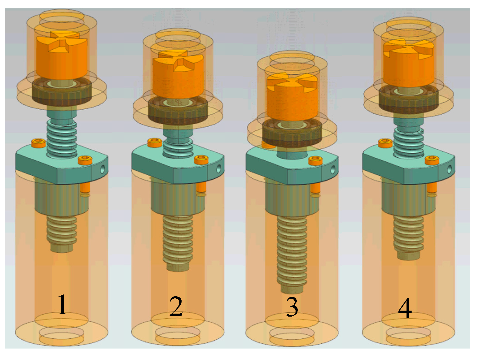
Figure 2.
ISD damping module.

Figure 3.
Vehicle model with ISD suspension.

Figure 4.
The fitting periodic road excitation model.

Figure 5.
The consecutive speed control humps model.

Figure 6.
Simulation condition schematic.

Figure 7.
The objective function value under fitting periodic road excitation.

Figure 8.
Dynamic characteristics under fitting periodic road excitation: (a) centroid acceleration; (b) pitch angular acceleration; (c) roll angular acceleration; (d) yaw angular acceleration; (e) suspension working space; (f) tyre dynamic load.
Figure 8.
Dynamic characteristics under fitting periodic road excitation: (a) centroid acceleration; (b) pitch angular acceleration; (c) roll angular acceleration; (d) yaw angular acceleration; (e) suspension working space; (f) tyre dynamic load.


Figure 9.
The objective function value under consecutive speed control humps.

Figure 10.
Dynamic characteristics under consecutive speed control humps: (a) centroid acceleration; (b) pitch angular acceleration; (c) roll angular acceleration; (d) yaw angular acceleration; (e) suspension working space; (f) tyre dynamic load.
Figure 10.
Dynamic characteristics under consecutive speed control humps: (a) centroid acceleration; (b) pitch angular acceleration; (c) roll angular acceleration; (d) yaw angular acceleration; (e) suspension working space; (f) tyre dynamic load.
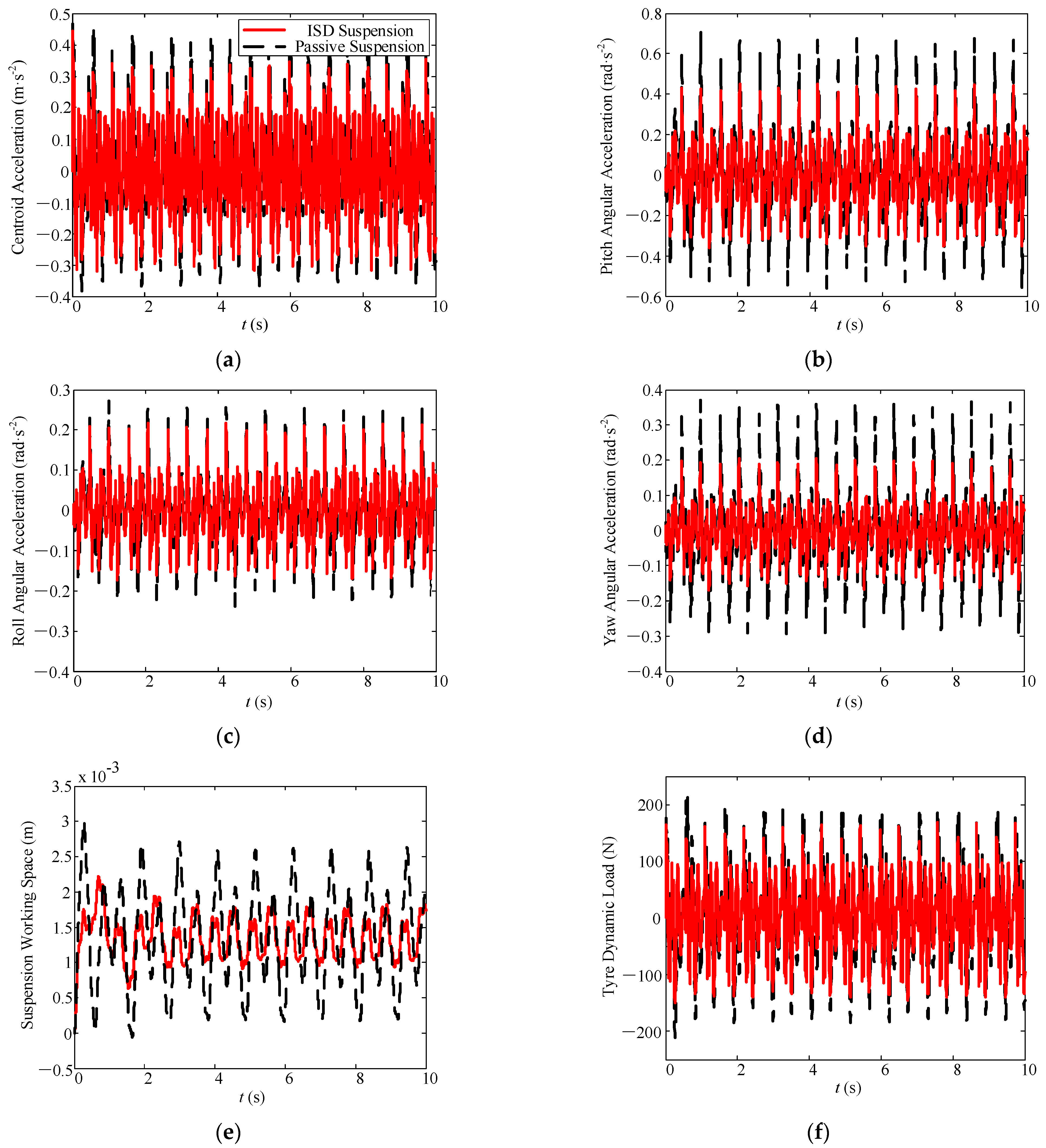
Figure 11.
The objective function value under coupled road excitation.

Figure 12.
Dynamic characteristics under coupled road excitation: (a) centroid acceleration; (b) pitch angular acceleration; (c) roll angular acceleration; (d) Yaw angular acceleration; (e) suspension working space; (f) tyre dynamic load.
Figure 12.
Dynamic characteristics under coupled road excitation: (a) centroid acceleration; (b) pitch angular acceleration; (c) roll angular acceleration; (d) Yaw angular acceleration; (e) suspension working space; (f) tyre dynamic load.


Figure 13.
Performance improvement under different road excitations.


Table 1.
Parameters of the vehicle model.
| Item | Notation | Value |
|---|---|---|
| Vehicle mass | m | 1500 kg |
| Vehicle body mass | ms | 1342 kg |
| Front non-spring-loaded mass | mu1, mu2 | 90 kg |
| Rear non-spring-loaded mass | mu3, mu4 | 70 kg |
| Body roll moment of inertia | Ix | 521 kg·m2 |
| Body pitch moment of inertia | Iy | 2436 kg·m2 |
| Body yaw moment of inertia | Iz | 2120 kg·m2 |
| Vehicle yaw moment of inertia | I | 2414 kg·m2 |
| Inertia product of body mass | Ixz | 1165 kg·m2 |
| Height from centroid to roll center | H | 0.083 m |
| Distance from the centroid of vehicle mass to body mass | Ls | 0.12 m |
| Distance from the front axle to the centroid | a | 1.219 m |
| Distance from the rear axle to the centroid | e | 1.252 m |
| Half tread of left and right wheels | d | 0.72 m |
| Spring stiffness of first stage suspension (1,2) | k11, k21 | 19 kN·m−1 |
| Spring stiffness of first stage suspension (3,4) | k31, k41 | 14.7 kN·m−1 |
| Damping coefficient of first stage suspension (1,2) | c11, c21 | 0.897 kN·s·m−1 |
| Damping coefficient of first stage suspension (3,4) | c31, c41 | 0.769 kN·s·m−1 |
| Tyre stiffness | k13, k23, k33, k43 | 150 kN·m−1 |
| Spring stiffness of second stage suspension (1,2,3,4) | k12, k22, k32, k42 | 10 kN·m−1 |
| Damping coefficient of second stage suspension (1,2) | c12, c22 | 1.194 kN·s·m−1 |
| Damping coefficient of second stage suspension (3,4) | c32, c42 | 1.068 kN·s·m−1 |
| Inertance of the front suspension | b1, b2 | 153 kg |
| Inertance of the rear suspension | b3, b4 | 136 kg |
Table 2.
Comparison of performance indicators under fitting periodic road excitation.
| Performance | Value | Passive Suspension | ISD Suspension | Decrease Ratios (%) |
|---|---|---|---|---|
| Centroid acceleration (m·s−2) | RMS | 2.7182 | 0.8155 | 70.0 |
| Peak | 4.9244 | 2.3082 | 53.1 | |
| Pitch angular acceleration (rad·s−2) | RMS | 3.8319 | 2.8658 | 25.2 |
| Peak | 7.5659 | 6.0220 | 24.9 | |
| Roll angular acceleration (rad·s−2) | RMS | 1.4627 | 1.3827 | 5.5 |
| Peak | 2.9197 | 2.9115 | 0.3 | |
| Yaw angular acceleration (rad·s−2) | RMS | 2.2076 | 1.2101 | 45.2 |
| Peak | 7.4196 | 2.5874 | 65.1 | |
| Suspension working space (m) | RMS | 0.0434 | 0.0084 | 80.6 |
| Peak | 0.0715 | 0.0218 | 69.5 | |
| Tyre dynamic load (N) | RMS | 1642.4 | 900.2 | 45.2 |
| Peak | 4784.7 | 1622.4 | 66.1 |
Table 3.
Comparison of performance indicators under consecutive speed control humps.
| Performance | Value | Passive Suspension | ISD Suspension | Decrease Ratios (%) |
|---|---|---|---|---|
| Centroid acceleration (m·s−2) | RMS | 0.1635 | 0.1417 | 13.3 |
| Peak | 0.4749 | 0.4421 | 6.9 | |
| Pitch angular acceleration (rad·s−2) | RMS | 0.2033 | 0.1359 | 33.2 |
| Peak | 0.7088 | 0.4481 | 36.8 | |
| Roll angular acceleration (rad·s−2) | RMS | 0.0779 | 0.0656 | 15.8 |
| Peak | 0.2717 | 0.2163 | 20.3 | |
| Yaw angular acceleration (rad·s−2) | RMS | 0.1067 | 0.0601 | 43.7 |
| Peak | 0.3709 | 0.2043 | 44.9 | |
| Suspension working space (m) | RMS | 0.0013 | 0.0012 | 7.7 |
| Peak | 0.0030 | 0.0022 | 26.6 | |
| Tyre dynamic load (N) | RMS | 73.78 | 55.89 | 24.2 |
| Peak | 212.1 | 168.2 | 20.7 |
Table 4.
Comparison of performance indicators under coupled road excitation.
| Performance | Value | Passive Suspension | ISD Suspension | Decrease Ratios (%) |
|---|---|---|---|---|
| Centroid acceleration (m·s−2) | RMS | 2.6075 | 0.9915 | 62.0 |
| Peak | 4.6425 | 1.9253 | 58.5 | |
| Pitch angular acceleration (rad·s−2) | RMS | 5.2220 | 2.8001 | 46.4 |
| Peak | 18.116 | 4.9786 | 72.5 | |
| Roll angular acceleration (rad·s−2) | RMS | 1.8531 | 1.3518 | 27.1 |
| Peak | 5.0138 | 2.4164 | 51.8 | |
| Yaw angular acceleration (rad·s−2) | RMS | 3.7834 | 1.2201 | 67.8 |
| Peak | 18.022 | 2.0781 | 88.5 | |
| Suspension working space (m) | RMS | 0.0401 | 0.0078 | 80.5 |
| Peak | 0.0810 | 0.0180 | 77.8 | |
| Tyre dynamic load (N) | RMS | 2075.8 | 859.83 | 58.6 |
| Peak | 7858.9 | 1647.0 | 79.0 |
Publisher’s Note: MDPI stays neutral with regard to jurisdictional claims in published maps and institutional affiliations. |
© 2021 by the authors. Licensee MDPI, Basel, Switzerland. This article is an open access article distributed under the terms and conditions of the Creative Commons Attribution (CC BY) license (https://creativecommons.org/licenses/by/4.0/).
Share and Cite
MDPI and ACS Style
Li, X.; Li, F.; Shang, D. Dynamic Characteristics Analysis of ISD Suspension System under Different Working Conditions. Mathematics 2021, 9, 1345. https://doi.org/10.3390/math9121345
AMA Style
Li X, Li F, Shang D. Dynamic Characteristics Analysis of ISD Suspension System under Different Working Conditions. Mathematics. 2021; 9(12):1345. https://doi.org/10.3390/math9121345
Chicago/Turabian StyleLi, Xiaopeng, Fanjie Li, and Dongyang Shang. 2021. "Dynamic Characteristics Analysis of ISD Suspension System under Different Working Conditions" Mathematics 9, no. 12: 1345. https://doi.org/10.3390/math9121345
Note that from the first issue of 2016, this journal uses article numbers instead of page numbers. See further details here.