
Selection of the Bandwidth Matrix in Spatial Varying Coefficient Models to Detect Anisotropic Regression Relationships

1
College of Mathematics and System Sciences, Xinjiang University, Urumqi 830046, China
2
College of Resources and Environmental Sciences, Xinjiang University, Urumqi 830046, China
*
Authors to whom correspondence should be addressed.
Mathematics 2021, 9(18), 2343; https://doi.org/10.3390/math9182343
Submission received: 7 July 2021
/
Revised: 6 September 2021
/
Accepted: 17 September 2021
/
Published: 21 September 2021
Abstract
:The commonly used Geographically Weighted Regression (GWR) fitting method for a spatial varying coefficient model is to select a bandwidth h for the geographic location (u, v), and assign the same weight to the two dimensions. However, spatial data usually present anisotropy. The introduction of a two-dimensional bandwidth matrix not only gives weight from two dimensions separately, but also increases the direction of kernel smoothness. The adaptive bandwidth matrix is more flexible. Therefore, in this paper, a two dimensional bandwidth matrix is introduced into the spatial varying coefficient model for parameter estimation. Through simulation experiments, the results obtained under the adaptive bandwidth matrix are compared with those obtained under the global bandwidth matrix, indicating the effectiveness of introducing the adaptive bandwidth matrix.
1. Introduction
The spatial varying coefficient model proposed by Brunsdon et al. (1996) [1] is a widely used and significant model in non-parametric statistics. It is a non-parametric smoothing method with the distance function between observation points as the weight.
The work of Brunsdon et al. (1998) [2] and Fotheringham et al. (1998) [3] shows the role of the Geographically Weighted Regression (GWR) method in studying the nonstationarity of spatial data regression relationships, and the effectiveness of the method was demonstrated through actual data. Since the two-dimensional region is larger than the one-dimensional region, it is easy to produce boundary effects. Wang et al. (2008) [4] extended the local linear fitting method from the varying coefficient model to the spatial varying coefficient model, and proposed the local linear GWR method. Recently, the backfitting technique has been successfully applied to the GWR models for dealing with the multiscale issue by manipulating the bandwidth in the kernel function (Fotheringham et al. (2017) [5], Leong and Yue (2017) [6], Yu et al. (2020) [7]). The kernel smoothing method is an effective method for solving non-parametric problems, in which the selection of the bandwidth h is more important than the selection of the kernel function itself. For the selection of bandwidth, the cross-validation method (CV) and its variants are widely used in practice, such as the generalized cross-validation method (GCV), or the AICc method to select the optimal bandwidth. If the estimated curve is smooth, the global bandwidth can be selected; while if the estimated curve has a complex structure, the adaptive bandwidth can be considered. There are two important studies on adaptive bandwidth: one is the K-nearest neighbor method proposed by Loftsgaarden and Quesenberry (1965) [8]; the second is the adaptive kernel density estimation proposed by Breiman et al. (1977) [9]. Subsequently, ref. [10] proposed using the square root method to select the adaptive bandwidth, that is, for any dimension, the bandwidth in the form can be selected. Fan and Gijbels (1995) [11] used a data-driven method to select the bandwidth; based on the estimated curvature, they proposed a new method for estimating the approximate deviation and variance of local polynomial fitting. Tian (2019) [12] used the cutting-edge knowledge of statistics to research the four major contemporary non-parametric statistics in the selection of bandwidth.
Many studies are limited to one-dimensional cases, while non-parametric problems will have more important applications in higher dimensions. The bandwidth matrix obtained under high-dimensional data not only affects the smoothness, but also affects the smoothing direction. For high-dimensional data, there are mainly the Plug-in insertion method, SCV and other methods for selecting the bandwidth matrix (Gramacki (2018) [13], Chacón and Duong (2018) [14]). Among them, the Plug-in insertion method is more stable for selecting bandwidth matrix H.
Wand and Jones (1994) [15] used the Plug-in method for multi-dimensional data to select a constrained bandwidth matrix. Duong and Hazelton (2003) [16] used the Plug-in method to select a binary unconstrained bandwidth matrix. Subsequently, Chacón and Duong (2010) [17] improved it by selecting unconstrained bandwidth matrix for high-dimensional data. In addition, the Bayesian method is also applied to the field of bandwidth selection. There are also many ways to select high-dimensional bandwidths by using the prior information from the data.
Brewer (2000) [18] proposed a new method for adaptive bandwidth in univariate kernel density estimation based on likelihood cross-validation and Bayesian graphical model analysis. Zhang et al. (2006) [19] took the bandwidth matrix elements as the parameters, and the posterior density was obtained by the Likelihood Cross-Validation criterion. The optimal window width was estimated by MCMC algorithm. Zougab et al. (2014) [20] used Bayesian estimation method to select adaptive bandwidth matrix, and so forth. For multi-dimensional data, besides bandwidth matrix, the product kernel is usually used to solve high-dimensional problems. Belaid et al. (2018) [21] applied the adaptive bandwidth selected by the Bayesian method to the high-dimensional discrete kernel. Gramacki and Gramacki (2017) [22] used the FFT method to solve some problems of the bandwidth matrix.
Sain et al. (1994) [23] used the CV method to select multiple bandwidths by the form of the product kernel. Wu et al. (2007) [24] regard the local bandwidth as the product of the local bandwidth factor and the global bandwidth, calculate the local window width factor with the clustering analysis algorithm, and obtain the multiple adaptive bandwidth. However, the kernel form of the multivariate product is essentially similar to the diagonal matrix. Xu (2009) [25] extended the bandwidth h of the coefficient function in the varying coefficient model to multidimensional, and theoretically tried to give a diagonal bandwidth matrix, where the values of diagonal elements were consistent. Wand and Jones (1993) [26] believe that the unconstrained bandwidth matrix is more general than the diagonal bandwidth matrix, and is applicable to a wider range. Unconstrained matrices can include many more smooth directions.
In many practical fields, such as geography, ecology, and meteorology, the data obtained usually contain geographic location information, and this kind of data is called spatial data. Spatial effects mainly come from spatial dependence (that is, spatial correlation) and spatial heterogeneity (that is, spatial non-stationarity). The spatial data are usually not in the same quantity distribution in all directions of geographical position, and the data distribution is not uniform, showing anisotropy. At present, there is no good way to deal with this phenomenon. The local linear geographically weight regression method is usually adopted to solve the fitting problem of the spatial variable coefficient model. In this method, the distance function between observation points is usually used as the weight value, and the same window width h is selected for the geographical position (u, v), that is, the data of two dimensions are given the same weight as isotropy. Considering the spatial anisotropy and dependence of the two variables (u, v), this paper introduces the two-dimensional Gaussian kernel function into the coefficient function estimation of the spatial variable coefficient model, and uses the binary unconstrained bandwidth matrix H to select different bandwidths from the two dimensions of geographical location, u and v. This can increase the direction of the smooth kernel, which can also explain the anisotropy. Furthermore, the adaptive bandwidth matrix is studied, and the coefficient estimates of the spatial variable coefficient models of the binary bandwidth matrix and the adaptive window width matrix are obtained respectively. Through simulation experiments, it is shown that the introduction of adaptive bandwidth matrix is more effective and flexible than the global bandwidth matrix.
2. Selection and Estimation of Bandwidth of Spatial Varying Coefficient Model
2.1. Spatial Varying Coefficient Model
The spatial varying coefficient model is to embed the data with the geographical location information into the varying coefficient model, which can not only avoid the dimensional disaster problem in fitting, but can also well reflect the spatial non-stationary and heterogeneous characteristics of the regression relationship. The specific form of the spatial varying coefficient model is as follows:
where represents the observed value of the dependent variable and independent variable at the geographic location, , is a function of geographic location, and is the error term, which satisfies . The model allows a spatially varying interception by setting .
Brunsdo et al. [1] explicitly gave the specific form of the spatial varying coefficient model for the first time and proposed a method using the distance function between observation points as the weight, namely the geographically weighted regression method, which essentially belongs to the Nadaraya–Watson kernel estimation method. The boundary effects exists in this method, while the boundary of the two-dimensional geographic region is larger than that of the one-dimensional region, and the data of the boundary region is more prone to distortion. The local polynomial fitting method can automatically correct the boundary effect (Mei and Wang (2012) [27]). Wang et al. (2008) [4] extended the local linear fitting method from the varying coefficient model to the spatial varying coefficient model, and presented the locally linear GWR method. In order to avoid the boundary effects, the local linear GWR method is used for model fitting in this paper.
For a given location in the studied area, the estimates of at , and the matrix notation as follows:
where is the p-order identity matrix and is the p-order zero matrix, and is the observations vector of the response variable. The design matrix at point is:
and is a diagonal weight matrix with , is a kernel function. The kernel functions used in this paper are all Gaussian kernel functions. For the traditional GWR method, the specific form of the one-dimensional Gauss kernel function is as follows:
where, represents the Euclidean distance between and Specifically, the set of weights at in Equation (2) are
The specific form of the two-dimensional Gauss kernel function is as follows:
The set of weights at is The spatial varying coefficient model involves two variables, u and v, so is a binary vector about u and v, is a binary bandwidth matrix about , the distance used here is formally known as the Mahalanobis distance.
The estimate of the dependent variable is:
where is the hat matrix. The hat matrix used for parameter estimation using the one-dimensional kernel function has the following form:
The hat matrix used in parameter estimation using two-dimensional kernel function has the following form:
2.2. Selection of Bandwidth Matrix
(1) The bandwidth matrix of the unary variable is , Here, the square of the window width is used to consider the problem. In this paper, the generalized cross validation method (GCV) is used to select the one-dimensional bandwidth in traditional GWR method:
where L is the hat matrix, represents the trace of the matrix, represents the value of the ith dependent variable, . To select the optimal window width , in practical application, a range is first given in accordance with a certain step size, the corresponding GCV(h) value is calculated, and the that makes GCV(H) reach the minimum is chosen, that is, , then is the selected optimal bandwidth.
(2) The form of the binary unconstrained window width matrix is as follows: , H is a symmetric positive definite matrix, . For the selection of the binary unconstrained bandwidth matrix H, the Plug-in method proposed by Duong and Hazelton (2003) [16] is used for reference in this paper. The Plug-in method mainly relies on replacing the unknown function by the estimator in approximation, so that the asymptotic expression AMISE (Asymptotic Mean Integrated Squared Error) of the estimated MISE (Mean Integrated Squared Error) can reach the minimum value. Here, t can be regarded as a set of data about u and v, and f(t) is the target density function. The specific expressions of MISE and AMISE are as follows:
where , , , represents a special form of column vector, for example, = .
Then is a 3 × 3 matrix, the specific form is as follows:
is the Hessian matrix of f, and denotes the diagonal matrix formed by replacing all off-diagonal entries of A by zeroes. are integrals of products of density derivatives of .
To obtain the optimal bandwidth matrix H, the key is to estimate . The elements in are , , , , are non-negative integers, is the r-order partial derivative with respect to . Firstly, the original data are standardized, and the test bandwidth matrix G is used to replace H to estimate each element in , separately:
Calculate the variance and deviation of related G. Let . Since g is also unknown, calculate the variance and deviation of g to obtain the AMSE related to g:
represents the unit vector whose ith value is 1, and sum over all to get .
To take the g which minimizes . Here, the final bandwidth matrix H is generally obtained by the two-stage method. The selection of the optimal bandwidth matrix can be implemented in the “ks” package of the R language.
(3) As for the selection of the adaptive bandwidth matrix, the Bayesian method proposed by Zougab et al. (2014) [20] was adopted in this paper. Under the Bayesian framework, the prior distribution is selected as the conjugate prior distribution, and the explicit expression of the adaptive window width matrix is obtained by combining with the square loss function. Here, t can be viewed as a set of data about u and v. The specific calculation steps are as follows: the kernel estimation is carried out by leave-one out method estimation.
The kernel function generally uses Gaussian kernel:
At this time, its prior distribution can take its conjugate prior distribution, that is, the inverse Wishard prior distribution,
where is the classic Gamma function.
Under the square loss function, the explicit expression of a posteriori estimate can be given, which can avoid the consumption of a lot of operation time during sampling calculation. For each bandwidth matrix , the form of a posteriori probability is as follows:
The posterior distribution can be expressed as follows:
For each j term in the posterior distribution, where is multiplied by something with unit 1, where the quantity with unit 1 can be expressed as:
Then, we can get:
where r is the degree of freedom, given , Q is the covariance matrix of the sample. For the adaptive bandwidth matrix, the specific form of the two-dimensional Gauss kernel function is as follows:
The set of weights at is here is a binary vector about is a binary bandwidth matrix about . The corresponding hat matrix L has the following forms:
3. Simulation Experiment
In order to reflect the spatial scale difference and interdependence between , both and are taken as n sample points on uniformly distributed of , and set the matrix and . By rotating , a set of geographic locations with relevant relationships is obtained. The rotated was used in the experiment to reflect the spatial scale difference and the dependent relationship between the geographical positions of the spatial data.
The model used to generate spatial data is as follows:
where the independent variable is a column vector of all 1, that is, the observation values are all 1, and the observation values are independent values generated from the uniform distribution U(0,2), the error are n independent and identically distributed random numbers that obey the normal distribution , where the sample size is taken as , let , and the real surfaces are shown in Figure 1.
The coefficient functions in Equation (19) are calibrated by the Formula (2), and the optimal bandwidth in the kernel function is selected in three ways: the GCV-based method in Equation (8), the Plug-in-based matrix H method in Equation (11) and the adaptive bandwidth matrix H method in Equation (16). We get the GCV-based optimal bandwidth , and the Plug-in-based optimal bandwidth matrix H is . The accuracy of parameter estimation is evaluated by the mean square error (MSE). Its definition is ; the smaller the value of the , the better the fitting effect. In order to compare the performance of the above three estimation methods, keep other quantities fixed, re-sample data with a sample size of n from , do repeated experiments, calculate the of , , and take the average of the N replications. The numerical results are shown in the Table 1. Additionally, Figure 2 and Figure 3 display the estimated coefficients and the estimation residuals of and with the GCV-based bandwidth, the bandwidth matrix and the adaptive bandwidth matrix method, respectively.
It can be found from the simulation results in Table 1 that the MSE of regression coefficients estimation obtained by using the bandwidth matrix H and the adaptive bandwidth matrix are smaller than that obtained by using GCV-based bandwidth h for 200 replications. The parameter estimation MSE of and obtained by the adaptive bandwidth matrix is less than that of the parameter estimation of and obtained by the direct use of the bandwidth matrix. In other words, the estimation result obtained by the adaptive bandwidth matrix is better than that obtained by the use of the bandwidth matrix. That means the performance of two dimensions’ unconstrained bandwidth matrix for geographical location is better than that of selecting one bandwidth for two variables in the spatially varying coefficient model. In addition, when the bandwidth matrix H obtained by the Plug-in method is used for parameter estimation, the running time of the program is shorter than that obtained by the GCV-based method.
From the residual graph of the coefficient function in Figure 2 and Figure 3, the estimated residuals are dispersed by selecting the same bandwidth h for u and v, and the estimated residuals are relatively concentrated around zero by selecting the bandwidth matrix H, although there are a few points with large differences. The residuals boxplots of in Figure 2 and in Figure 3 show that the estimated residuals of are more concentrated by using the adaptive bandwidth matrix than the global bandwidth matrix. The reason for the occurrence of large bias points may be related to the non-diagonal elements of the bandwidth matrix H, or an adaptive bandwidth matrix can be introduced. The introduction of the adaptive bandwidth matrix can reduce the outliers. It further proves the effectiveness of introducing a two-dimensional adaptive bandwidth matrix into the spatial varying coefficient model.
The above results show that, in the spatial varying coefficient model, considering the spatial anisotropy and correlation of spatial coordinates , the estimated coefficient surfaces obtained by selecting bandwidth matrix H is more accurate than that obtained by selecting the same bandwidth h for the two spatial coordinates . In addition, compared with GCV-based method, using the Plug-in-based method to select the bandwidth matrix can reduce the number of iterations in model fitting and improve computational efficiency.
4. Empirical Research
The Fractional Vegetation Cover (FVC) quantifies the denseness of vegetation and reflects the growth trend of vegetation. FVC plays an important role in reflecting the process of climate change and is an important indicator of ecological environmental change and is a useful parameter for many environmental and climate-related applications. In this research, the datasets of variables FVC, temperature and precipitation in Yili, Xinjiang were collected to study the spatial varying relationships between FVC and climate factors.
4.1. Data Sources
Yili Kazakh Autonomous Prefecture was the selected research area, located in northwest China’s Xinjiang Uygur Autonomous Region, surrounded by mountains, and vulnerable to influence of airflow around the Tianshan mountains, the Wusun mountain, Kequqin and the Nalati mountain. Inside the Yili river near the Yili river valley, there is a humid climate and abundant rainfall; it is arguably the wettest region in Xinjiang. In this paper, the data on air temperature, precipitation and FVC in Yili, Xinjiang in 2011 adopted by Feng et al. (2016) [28] were used, with a total of 835 corresponding data points.
4.2. Modelling
The specific form of the spatial varying coefficient model in this section is as follows:
where represents the observation value of the ith vegetation coverage index, is always equal to 1, represents the observation value of the ith annual average precipitation, and represents the observation value of the ith annual average temperature, represents the benchmark vegetation coverage index, represents the influence intensity of the annual average precipitation at the ith point on the vegetation coverage index, represents the intensity of influence of the annual average temperature at the ith point on the vegetation coverage index, represents the residual. For the estimation of the coefficient function, the local linear GWR method is used for model fitting and parameter estimation.
4.3. Results and Analysis
4.3.1. Results of Unary Bandwidth and Bandwidth Matrix
According to the method of selecting the bandwidth matrix introduced in Section 2.2, the bandwidth h = 12,938.16 and the bandwidth matrix , according to formulas in Equations (3) and (4), a one-dimensional kernel function and a two-dimensional kernel function, are constructed to fit the model respectively and to obtain the MSE of the estimated value of the dependent variable and the running time of the program. The results in Table 2 show that the MSE(Y) obtained by the two-dimensional kernel function with the bandwidth matrix is smaller, the estimation is more accurate, the program running time is greatly shortened, and the running efficiency is greatly improved.
The estimated values obtained from the bandwidth matrix H in Table 3 show that: the coefficient function and the coefficient function of annual mean temperature and precipitation both show obvious spatial and regional differences. There was a positive correlation between precipitation and FVC, and the regions with more precipitation had higher vegetation coverage. There was also a positive correlation between temperature and FVC.
The results in Figure 4 show that, in the spatial varying coefficient model, the estimated value obtained by selecting the binary bandwidth matrix H for the kernel function is roughly consistent with the real vegetation coverage index, and the residual is small. The vegetation coverage index in most areas of Yili is relatively high, while the vegetation coverage index in the border area and the northwest is slightly lower, which is consistent with the actual situation. The reasons for this phenomenon may be related to temperature, precipitation, terrain, and so forth. It should be noted that, in addition to intuitively exploring spatial varying regression relationships by summary tables or images of the estimated coefficient functions, the statistical inference methods can be used to test the significance of spatial non-stationary relationships, including the residual sum of square based statistics with an F-distribution (Leung et al., 2000 [29]; Mei et al., 2006 [30]) and the bootstrap methods (Wei and Qi 2012 [31]; Mei et al., 2016 [32]).
4.3.2. Results of Bandwidth Matrix and Adaptive Bandwidth Matrix
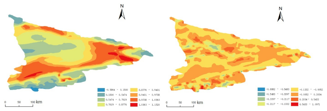
According to the adaptive bandwidth matrix H method discussed in Section 2, Equation (16), the estimated result of the coefficient function can be found in Table 4, and Figure 5 shows the prediction of the FVC and the residuals with the adaptive bandwidth matrix.
By observing the estimated values of the coefficient functions in Table 4, it is easy to see that the values of are mostly positive numbers. For and , most of the values are positive, that is, precipitation and temperature have a positive effect on the FVC. By comparing Table 3 and Table 4 we can find that, compared to the range of parameter estimates obtained with a fixed bandwidth matrix, the range of parameter estimates obtained by the adaptive bandwidth matrix is smaller.
5. Summary and Prospect
(1) When there is a scale problem and a correlation between two variables, that is, the smoothness between the two variables is different and there is anisotropy in space, it is more reasonable to consider the two variables in selecting the binary bandwidth matrix than to select the same bandwidth fitting value between the two variables. At the same time, as an intermediary between a one-dimensional univariate and a high-dimensional multivariate, a bivariate has a smoother direction than a univariate kernel, and is easy to visualize. This also makes it possible to generalize the spatio-temporal variable coefficient model to the unconstrained bandwidth matrix of the spatio-temporal variable coefficient model or an even higher dimensional bandwidth matrix.
(2) Compared with the GCV method, using the Plug-in method to select the bandwidth matrix can reduce the number of iterations in the process of selecting the optimal bandwidth h, and can shorten the iteration time of program operation and improve the efficiency of calculation.
(3) By observing the residuals of the parameter estimates, we find that the residual range of the parameter estimates obtained under the bandwidth is small, while most of the residual values of the parameter estimates obtained under the bandwidth matrix are very concentrated. It will have points with larger residual values, which may be related to non-diagonal elements. We can also try to add an adaptive bandwidth matrix, which is worth continuing to study.
Author Contributions
Conceptualization, X.H. and H.Z.; methodology, Y.L.; software, Y.L.; validation, X.H. and H.Z.; formal analysis, H.Z. and Y.L.; investigation, Y.L. and X.H.; resources, Q.S.; data curation, Q.S.; writing—original draft preparation, Y.L.; writing—review and editing, H.Z.; visualization, Y.L. and H.Z.; supervision, X.H. and H.Z.; project administration, H.J.; funding acquisition, X.H. All authors have read and agreed to the published version of the manuscript.
Funding
This study is supported by the National Natural Science Foundation of China grand number 11961065 and U1703237). Zhang’s work is also partially supported by the Natural Science Foundation of Xinjiang grant number 2019D01C045 and The Ministry of education of Humanities and Social Science project grant number 19YJA910007.
Institutional Review Board Statement
Not applicable.
Informed Consent Statement
Not applicable.
Data Availability Statement
The data in the paper can be requested by email to the corresponding author.
Conflicts of Interest
The authors declare no conflict of interest.
References
- Brunsdon, C.; Fotheringham, A.S.; Charlton, M.E. Geographically weighted regression: A method for exploring spatial nonstationarity. Geogr. Anal. 1996, 28, 281–298. [Google Scholar] [CrossRef]
- Brunsdont, C.; Fotheringham, S.; Charlton, M.E. Geographically weighted regression—Modelling spatial non-stationarity. J. R. Stat. Soc. Ser. D Stat. 1998, 47, 431–443. [Google Scholar] [CrossRef]
- Fotheringham, A.S.; Charlton, M.E.; Brunsdon, C. Geographically Weighted Regression: A Natural Evolution of The Expansion Method for Spatial Data Analysis. Environ. Plan. A 1998, 30, 1905–1927. [Google Scholar] [CrossRef]
- Wang, N.; Mei, C.L.; Yan, X.D. Local linear estimation of spatial varying coefficient models: An improvement on the geographically weighted regression technique. Environ. Plan. A 2008, 40, 986–1005. [Google Scholar] [CrossRef]
- Fotheringham, A.S.; Yang, W.; Kang, W. Multiscale Geographically Weighted Regression (MGWR). Ann. Am. Assoc. Geogr. 2017, 107, 1247–1265. [Google Scholar] [CrossRef]
- Leong, Y.Y.; Yue, J.C. A Modification to Geographically Weighted Regression. Int. J. Health Geogr. 2017, 16, 11. [Google Scholar] [CrossRef] [PubMed] [Green Version]
- Yu, H.; Fotheringham, A.S.; Li, Z.; Oshan, T.; Kang, W.; Wolf, L.J. Inference in multiscale geographically weighted regression. Geogr. Anal. 2020, 52, 87–106. [Google Scholar] [CrossRef]
- Loftsgaarden, D.O.; Quesenberry, C.P. A Nonparametric Estimate of a Multivariate Density Function. Ann. Math. Stat. 1965, 36, 1049–1051. [Google Scholar] [CrossRef]
- Breiman, L.; Meisel, W.; Purcell, E. Variable kernel estimates of multivariate densities. Technometrics 1977, 19, 135–144. [Google Scholar] [CrossRef]
- Abramson, I.S. On bandwidth variation in kernel estimates-a square root law. Ann. Stat. 1982, 10, 1217–1223. [Google Scholar] [CrossRef]
- Fan, J.; Gijbels, I. Data-driven bandwidth selection in local polynomial fitting: Variable bandwidth and spatial adaptation. J. R. Stat. Soc. Ser. B Methodol. 1995, 57, 371–394. [Google Scholar] [CrossRef]
- Tian, M.Z. Selection and Application of bandwidth in Modern Nonparametric Statistics; Science Press: Beijing, China, 2019; pp. 206–260. [Google Scholar]
- Gramacki, A. Nonparametric Kernel Density Estimation and Its Computational Aspects; Springer International Publishing: Cham, Switzerland, 2018; pp. 63–83. [Google Scholar]
- Chacón, J.E.; Duong, T. Multivariate Kernel Smoothing and Its Applications; CRC Press: Boca Raton, FL, USA, 2018; pp. 43–66. [Google Scholar]
- Wand, M.P.; Jones, M.C. Multivariate plug-in bandwidth selection. Comput. Stat. 1994, 9, 97–116. [Google Scholar]
- Duong, T.; Hazelton, M. Plug-in bandwidth matrices for bivariate kernel density estimation. J. Nonparametric Stat. 2003, 15, 17–30. [Google Scholar] [CrossRef]
- Chacón, J.E.; Duong, T. Multivariate plug-in bandwidth selection with unconstrained pilot bandwidth matrices. Test 2010, 19, 375–398. [Google Scholar] [CrossRef]
- Brewer, M. Bayesian model for local smoothing in kernel density estimation. Stat. Comput. 2000, 10, 299–309. [Google Scholar] [CrossRef]
- Zhang, X.; King, M.L.; Hyndman, R.J. A Bayesian approach to bandwidth selection for multivariate kernel density estimation. Comput. Stat. Data Anal. 2006, 50, 3009–3031. [Google Scholar] [CrossRef] [Green Version]
- Zougab, N.; Adjabi, S.; Kokonendji, C. Bayesian estimation of adaptive bandwidth matrices in multivariate kernel density estimation. Comput. Stat. Data Anal. 2014, 75, 28–38. [Google Scholar] [CrossRef]
- Belaid, N.; Adjabi, S.; Kokonendji, C.C.; Zougab, N. Bayesian adaptive bandwidth selector for multivariate discrete kernel estimator. Commun. Stat.-Theory Methods 2018, 47, 2988–3001. [Google Scholar] [CrossRef]
- Gramacki, A.; Gramacki, J. FFT-based fast computation of multivariate kernel density estimators with unconstrained bandwidth matrices. J. Comput. Graph. Stat. 2017, 26, 459–462. [Google Scholar] [CrossRef]
- Sain, S.R.; Baggerly, K.A.; Scott, D.W. Cross-validation of multivariate densities. J. Am. Stat. Assoc. 1994, 89, 807–817. [Google Scholar] [CrossRef]
- Wu, T.; Chen, C.; Chen, H. A variable bandwidth selector in multivariate kernel density estimation. Stat. Probab. Lett. 2007, 77, 462–467. [Google Scholar] [CrossRef]
- Xu, J. Generalized Spatial Variable Coefficient Model. Ph.D. Thesis, Hunan Normal University, Changsha, China, 2009. [Google Scholar]
- Wand, M.P.; Jones, M.C. Comparison of smoothing parameterizations in bivariate kernel density estimation. J. Am. Stat. Assoc. 1993, 88, 520–528. [Google Scholar] [CrossRef]
- Mei, C.L.; Wang, N. Modern Regression Analysis Method; Science Press: Beijing, China, 2012; pp. 163–190. [Google Scholar]
- Feng, J.; Zhang, H.; Hu, X. Spatial non-stationary characteristics of the impacts of precipitation and temperature on FVC: A case study of Yili River Valley, Xinjiang. Chin. J. Ecol. 2016, 36, 4626–4634. [Google Scholar]
- Leung, Y.; Mei, C.L.; Zhang, W.X. Statistical Tests for Spatial Nonstationarity Based on the Geographically Weighted Regression Model. Environ. Plan. A 2000, 32, 9–32. [Google Scholar] [CrossRef]
- Mei, C.L.; Wang, N.; Zhang, W.X. Testing the importance of the explanatory variables in a mixed geographically weighted regression model. Environ. Plan. A Econ. Space 2006, 38, 587–598. [Google Scholar] [CrossRef]
- Wei, C.H.; Qi, F. On the estimation and testing of mixed geographically weighted regression models. Econ. Model. 2012, 29, 2615–2620. [Google Scholar] [CrossRef]
- Mei, C.L.; Xu, M.; Wang, N. A bootstrap test for constant coefficients in geographically weighted regression models. Int. J. Geogr. Inf. Sci. 2016, 30, 1622–1643. [Google Scholar] [CrossRef]
Figure 1.
The real surface of the coefficient function (left) and (right).
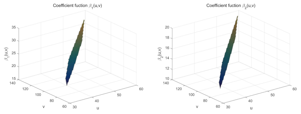
Figure 2.
The estimated surface of (top row) and residuals boxplots (bottom row) with the GCV−based method (left panel), the bandwidth matrix H (middle panel) and the adaptive bandwidth matrix H method (right panel).
Figure 2.
The estimated surface of (top row) and residuals boxplots (bottom row) with the GCV−based method (left panel), the bandwidth matrix H (middle panel) and the adaptive bandwidth matrix H method (right panel).
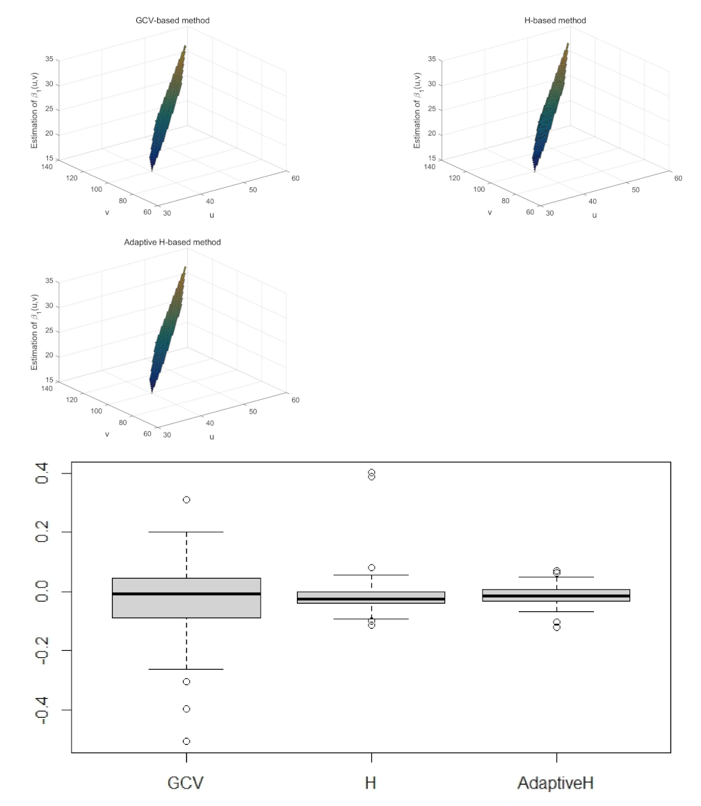
Figure 3.
The estimated surface of (top row) and residuals boxplots (bottom row) with the GCV−based method (left panel), the bandwidth matrix H (middle panel) and the adaptive bandwidth matrix H method (right panel).
Figure 3.
The estimated surface of (top row) and residuals boxplots (bottom row) with the GCV−based method (left panel), the bandwidth matrix H (middle panel) and the adaptive bandwidth matrix H method (right panel).
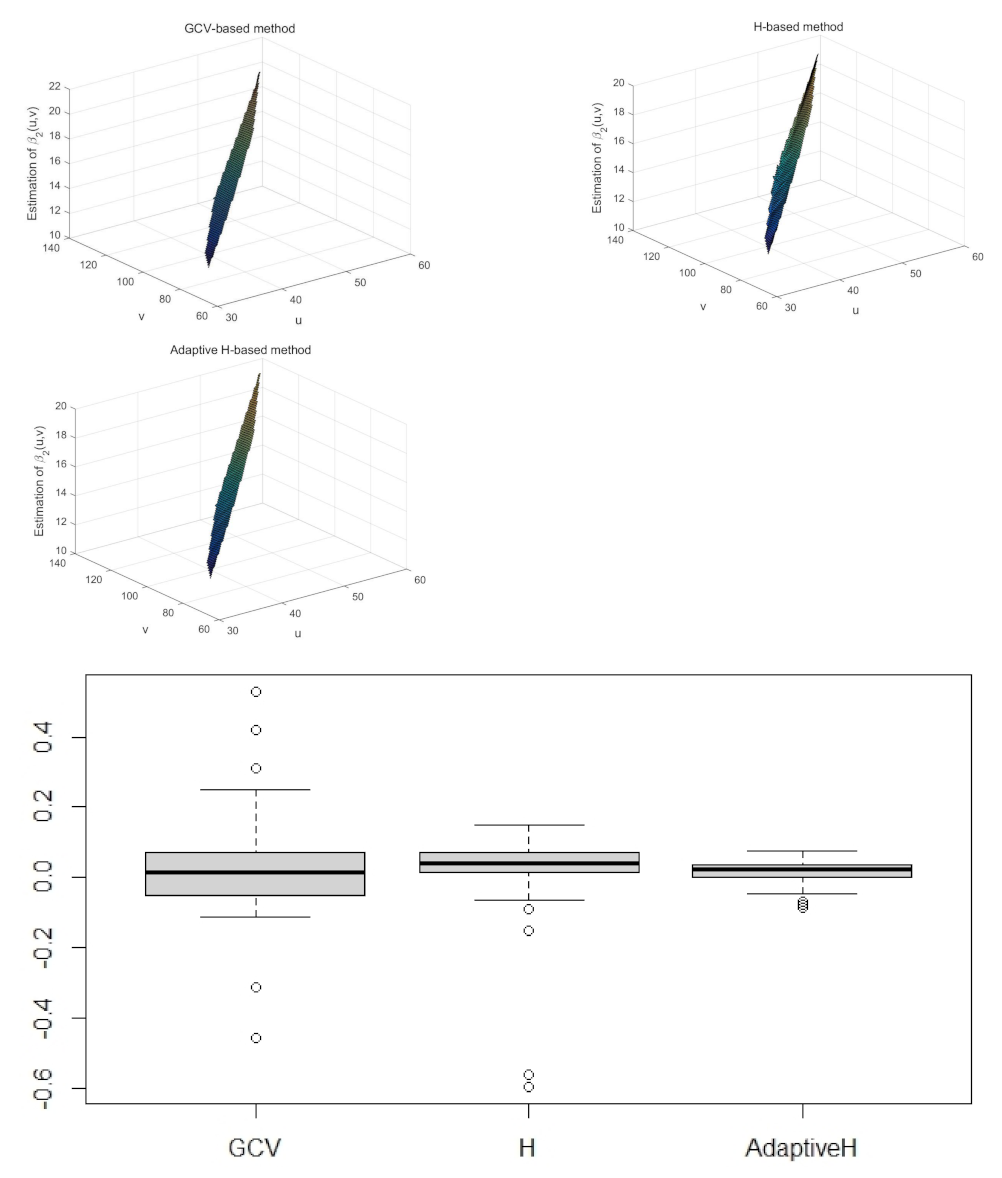
Figure 4.
Contour oftrue FVC in the research area (top row); The estimated contour and the residual of the FVC with bandwidth matrix H (bottom row).
Figure 4.
Contour oftrue FVC in the research area (top row); The estimated contour and the residual of the FVC with bandwidth matrix H (bottom row).
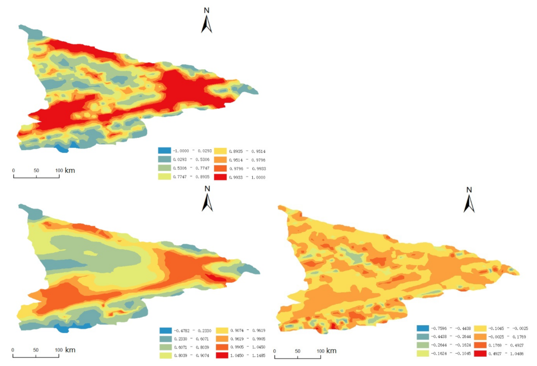
Figure 5.
The estimation of the FVC with the adaptive bandwidth matrix H (left) and the residuals (right).
Figure 5.
The estimation of the FVC with the adaptive bandwidth matrix H (left) and the residuals (right).

Table 1.
MSE results of the GCV-based bandwidth h, the bandwidth matrix H and the adaptive bandwidth matrix for N = 200 replications.
Table 1.
MSE results of the GCV-based bandwidth h, the bandwidth matrix H and the adaptive bandwidth matrix for N = 200 replications.
| Bandwidth Type | GCV-Based | Matrix H-Based | Adaptive Matrix H-Based |
|---|---|---|---|
| MSE(Y) | 3.0298 | 2.3928 | 0.6633 |
| MSE() | 0.0048 | 0.0136 | 0.0011 |
| MSE() | 0.0105 | 0.0137 | 0.0012 |
| Running time | 14.24 s | 2.38 s | 5.67 s |
Table 2.
Selected bandwidth and results of MSE.
| Bandwidth Type | Bandwidth h | Bandwidth Matrix H |
|---|---|---|
| MSE(Y) | 0.074 | 0.039 |
| Running time | 33.69 min | 1.32 min |
Table 3.
Regression coefficients estimation with bandwidth matrix H.
| Regression Coefficients | Minimum | 1/4 Quantile | Median | 3/4 Quantile | Maximum |
|---|---|---|---|---|---|
| −10.5274 | −0.0085 | 0.8041 | 1.3285 | 12.5262 | |
| −0.0349 | −0.0017 | 0.0003 | 0.0021 | 0.0358 | |
| −0.0788 | 0.0013 | 0.0155 | 0.0566 | 0.3834 |
Table 4.
Regression coefficients estimation with the adaptive bandwidth matrix H.
| Regression Coefficients | Minimum | 1/4 Quantile | Median | 3/4 Quantile | Maximum |
|---|---|---|---|---|---|
| −5.3196 | 0.3858 | 0.8049 | 1.1690 | 6.6727 | |
| −0.0207 | −0.0011 | 0.0002 | 0.0013 | 0.0196 | |
| −0.0288 | −0.0008 | 0.0141 | 0.0520 | 0.2599 |
Publisher’s Note: MDPI stays neutral with regard to jurisdictional claims in published maps and institutional affiliations. |
© 2021 by the authors. Licensee MDPI, Basel, Switzerland. This article is an open access article distributed under the terms and conditions of the Creative Commons Attribution (CC BY) license (https://creativecommons.org/licenses/by/4.0/).
Share and Cite
MDPI and ACS Style
Hu, X.; Lu, Y.; Zhang, H.; Jiang, H.; Shi, Q. Selection of the Bandwidth Matrix in Spatial Varying Coefficient Models to Detect Anisotropic Regression Relationships. Mathematics 2021, 9, 2343. https://doi.org/10.3390/math9182343
AMA Style
Hu X, Lu Y, Zhang H, Jiang H, Shi Q. Selection of the Bandwidth Matrix in Spatial Varying Coefficient Models to Detect Anisotropic Regression Relationships. Mathematics. 2021; 9(18):2343. https://doi.org/10.3390/math9182343
Chicago/Turabian StyleHu, Xijian, Yaori Lu, Huiguo Zhang, Haijun Jiang, and Qingdong Shi. 2021. "Selection of the Bandwidth Matrix in Spatial Varying Coefficient Models to Detect Anisotropic Regression Relationships" Mathematics 9, no. 18: 2343. https://doi.org/10.3390/math9182343
Note that from the first issue of 2016, this journal uses article numbers instead of page numbers. See further details here.