
Spatio-Temporal Spread Pattern of COVID-19 in Italy


Dipartimento di Scienze Economiche, Aziendali e Statistiche, Università degli Studi di Palermo, 90128 Palermo, Italy
*
Author to whom correspondence should be addressed.
Mathematics 2021, 9(19), 2454; https://doi.org/10.3390/math9192454
Submission received: 31 August 2021
/
Revised: 20 September 2021
/
Accepted: 26 September 2021
/
Published: 2 October 2021
(This article belongs to the Section Probability and Statistics)
Abstract
:This paper investigates the spatio-temporal spread pattern of COVID-19 in Italy, during the first wave of infections, from February to October 2020. Disease mappings of the virus infections by using the Besag–York–Mollié model and some spatio-temporal extensions are provided. This modeling framework, which includes a temporal component, allows the studying of the time evolution of the spread pattern among the 107 Italian provinces. The focus is on the effect of citizens’ mobility patterns, represented here by the three distinct phases of the Italian virus first wave, identified by the Italian government, also characterized by the lockdown period. Results show the effectiveness of the lockdown action and an inhomogeneous spatial trend that characterizes the virus spread during the first wave. Furthermore, the results suggest that the temporal evolution of each province’s cases is independent of the temporal evolution of the other ones, meaning that the contagions and temporal trend may be caused by some province-specific aspects rather than by the subjects’ spatial movements.
1. Introduction
The coronavirus SARS-CoV-2 (COVID-19) and the triggered disease were unknown before the outbreak began in Wuhan, China, in December 2019, and spread worldwide quickly. COVID-19 was declared a public health emergency of international concern (PHEIC) in January 2020, and Italy was the first and most affected European country during the first wave. Indeed, spatial-temporal information on the spread of the virus is of paramount importance for policy decision-makers.
Recent studies show the relevance of accounting for spatial and temporal patterns to explain and model the evolution of the pandemic with greater accuracy [1,2,3,4,5,6]. Refs. [7,8] deal with the outbreak and spread of the COVID-19 at a national level and global scale, respectively. Both of these papers describe the geographical distribution of the COVID-19 observations. Ref. [9] studies the epidemic spread in Iran through linear spatial models to identify the variables that have significantly impacted the virus infections size. Several authors have resorted to complex epidemiological SIR models. See, for example, Refs. [10,11,12,13], to name a few.
Unfortunately, the poor quality of public data, only available at the area level, limits the description of the spatial-temporal evolution of the virus’s spread. Ref. [14] states that, despite involving many excellent models, best intentions, and highly sophisticated tools, forecasting efforts have largely failed. the authors blame poor data input about critical features of the pandemic, which can heavily bias these estimates, exposing the reliability of any theory-based forecasting effort. Nevertheless, epidemic forecasting is unlikely to be abandoned. As discussed in [15], this paper focuses on the COVID-19 data limitations terms of availability and quality. This key aspect may be limiting for carrying out conclusive studies for this worldwide issue (see also [16] for more details). Moreover, the COVID-19 diffusion in Italy from February to October 2020, is modeled by the Besag–York–Mollié (BYM) model [17] and its spatio-temporal formulation.
This model has been applied also in disease mapping for areal aggregated data [18,19], supplying risk surfaces and spotting high-risk areas or hot-spots. Roughly speaking, spatial models can be distinguished into continuous and discrete domain models. Both classes of models are extensively considered in disease mapping. Indeed, calculating and visualizing disease risk across space is of paramount importance in epidemiology. When point-referenced data are available, Log–Gaussian Cox processes (LGCPs) are often applied as continuous domain models [20]. If point data are not available, models for areal data are the best choice. the Besag–York–Mollié (BYM) model, a discrete domain model, can be used to describe count data per spatial unit.
The BYM model represents a particular case of the LGCP, with piecewise constant relative risk within regions [21]. A methodology for describing aggregated disease incidence data with spatially continuous LGCP is proposed in [22], including an augmentation step sampling from the exact locations’ posterior distribution of an MCMC algorithm.
The BYM model accounts also for the neighborhood structure of the available count data, modeling the number of cases per district (denoting the general spatial unit), identifying the high-risk areas. the spatio-temporal extension of the BYM model, accounting also for the temporal domain, explores whether it is possible to highlight any specific evolution of the risk disease among the different phases of the Italian virus first wave.
The paper is structured as follows. Section 2 contains a discussion on the issues of the Italian COVID-19 data. Section 3 introduces the spatial and spatio-temporal models for areal data. in Section 4, we apply these models to the spread of COVID-19 infections in Italy from February to October 2020. in particular, Section 4.2 focuses on the Northern Italy regions, to assess the efficacy of the lockdown action in March 2020. Then, in Section 4.2 spatio-temporal models are fitted for all the Italian provinces, For assessing the effectiveness of the Italian Government restricting actions, that have characterized the Italian COVID-19 first wave. Finally, Section 5 outlines some future hints.
2. Concerns Related to the Italian COVID-19 Data
The Civil Protection publishes the COVID-19 Italian data as aggregated and reports the infected counts for regions and provinces every day. Unfortunately, these data present several issues that severely affect their quality. Firstly, there is no unique protocol for data transmission, so each regional healthcare organization has a different collection system. This lack of homogeneity may influence the reliability and makes their comparison in time and space difficult or even useless. the data issues can be broadly classified into delays in reporting cases, lack of comparable data, and time-varying under-reporting of COVID-19 cases.
- Delays in reporting cases. These occur because counts are updated on the notification day rather than aligned to a more appropriate date. Deaths may be counted on the day of the reporting instead of on the day of the outcome, and positive status may also be counted when test results are received, with swabs being done from one day to weeks after symptoms’ onset. Moreover, the reporting procedure may differ from area to area, making the data not comparable in space;
- Lack of comparable data. In Italy, up to the end of April 2020, only the total number of daily positive swabs were available, with neither information on swabs or tested individuals. This information would have been essential to use the swabs’ count to model the whole first pandemic wave;
- Time-varying under-reporting of COVID-19 cases. It is well established that people diagnosed with COVID-19 disease are only a tiny fraction of the infected ones. the swabs’ count changes over time since the tracking was highly symptoms’ driven in the first phase of the outbreak, and it continued to change following the different policies adopted. in particular, the swabs’ count has continued to increase significantly due to the increased availability of swabs since they became crucial for determining local government actions.
Following these considerations, our analysis focuses on a limited time interval, which corresponds to the first infection wave, to give an insight into the spatio-temporal spread of the COVID-19 in Italy, without explicitly inferring results. This time interval, which goes from February to October 2020, is divided into three phases identified by the Italian government, and some temporal indicators of the pandemic are aggregated accordingly. Specifically, we focus on the number of daily positives (i.e., people infected), which is an incidence indicator. Although being measured with some errors, these measurements still represent important indicators for monitoring of the pandemic [23]. Finally, we do not consider external covariates in the models, since our aim is not to identify the evolution determinants of the pandemic in Italy. Indeed, this ambitious task would require homogeneity and quality data, which is today still unavailable. In this regard, a COVID-19 dataset containing the number of daily cases registered in the regions of Catalonia (Spain), since the pandemic beginning to the end of August 2020, is analyzed in [24], by statistical models of different levels of complexity. The author shows that the choice of a specific statistical model may have a severe impact on the inferred associations between the covariates and the response variable. However, the author demonstrates that proper spatio-temporal models are helpful for the comprehension of the pandemic evolution both in space and time.
3. Spatial and Spatio-Temporal Models for Disease Mapping
The BYM model extends the intrinsic conditional autoregressive (ICAR) model, obtained by adding spatially unstructured random effects to the spatially structured ones. The latter is a realization of a Gaussian Markov random field (GMRF) with zero mean and a sparse precision matrix capturing strong spatial dependence. The unstructured random effect can be considered as a set of independent random intercepts associated to the areal units. Therefore, a piecewise constant risk surface can be considered, depending on the selected spatial unit, assuming that the risk is uniform across that unit.
Let be a random variable denoting the number of cases in the region , and the expected cases count for the i-th spatial unit, computed externally through population’s information. The number of expected cases can be obtained in several ways. For count data, expected rates for the disease of interest can be based on the age–sex structure of the local population. Refer to [25] or [26] for further proposed estimators of . The BYM model, in its general form, is defined as:
One advantage of the BYM model is the possibility to account for further external potential risk factors introduced as additive covariates. Here is a vector of area-level covariates with coefficients , and is the intercept representing the average areas counts. The random spatial process is obtained as the sum of two effects specific of the area, and . In particular, the former is an independent Gaussian process with variance , and the latter is a GMRF with variance . For each area, the value of the GMRF component depends on the average from the neighboring areas
where are all the area-specific effects except the i-th, denotes that areas i and j are neighbors, and is the number of areas sharing boundaries with the i-th one. Before estimating the model, we have to assign the set of the borough neighbors, considering the graph from a shapefile with information on all the area boundaries. We define neighboring districts if they share a common border, but weighted options are also possible, as the variance-stabilizing coding scheme proposed by [27], and the proposal of [28], dividing the weights by the minimum of the maximum-row-sums and maximum-column-sums. The parameter represents the unstructured residual, modeled as
When the ratio increases, the random spatial dependence rises up as well, providing a smoother surface for the intensity.
However, Ref. [29] note that this specification is not correct without previously scaling the precision matrix of the spatially structured random effect, and that the variance components in the BYM model are not identifiable from the data. See also [30]. Hence, only the sum is identifiable. For dealing with the identifiability issue, Ref. [31] proposed a modification of the BYM model. Ref. [32] addresses both the identifiability and scaling issue of the BYM model. More recently, [33] proposed a new parametrization of the BYM model called BYM2 which makes parameters interpretable and facilitates the assignment of meaningful penalized complexity (PC) priors [34]. The intrinsic Gaussian CAR prior results in a spatially smooth risk surface, which has the advantage of using information from multiple areas to estimate the random effects, but is not ideal if the aim is to identify clusters of high-risk areas [35]. Indeed, a cluster of areas with high risk may have low-risk neighbors, and, therefore, the estimated risk for these areas can be less visible using geographical smoothing [36].
The spatio-temporal disease mapping extension of the BYM model is widely used in disease surveillance studies [18,19]. In practice, the model in (1) is modified for accounting for a temporal component, which is indexed by . For each time t, either a parametric structure [37]
or a non parametric one [38]
can be specified for the log-intensity.
In practice, the term represents the temporally structured effect, added to the spatial effects and . the parameter can be modeled dynamically by a first (or second) order random walk, and it is defined as . Finally, is modeled with a Gaussian exchangeable prior .
The spatio-temporal model can be further extended to allow for interactions between space and time components, to study the evolution of the temporal trend among different areas, by
The parameter vector , containing all the , has a Gaussian distribution with a zero mean and a precision matrix given by where is an unknown scalar, while is a structure matrix, identifying the type of temporal and spatial dependence between the elements of [39].
Ref. [38] introduces four different types of specification for the precision matrix which implies different degree of prior dependence for the interaction parameters, and corresponds to the product of one of the two spatial with one of the two temporal main effects. Let ⊗ denotes the Kronecker product, we summarize the four different interpretations below, following [40].
- Type I assumes that the two unstructured effects and , give rise to the structure matrix , because both u and do not have a spatial or temporal structure. Consequently, we assume no spatial or temporal structure on the interaction either and, therefore, ;
- Type II combines the structured temporal main effect and the unstructured spatial effect . We write the structure matrix as where and is the neighborhood structure specified for instance through a first- or second-order random walk. This leads to the assumption that for the i-th area the parameter vector has an autoregressive structure on the time component, which is independent from the ones of the other areas;
- Type III combines the unstructured temporal effect and the spatially structured main effect . We write the structure matrix as , where and is a neighboring structure defined through the CAR specification. This leads to the assumption that the parameters of the t-th time point have a spatial structure independent from the other time points.
- Finally, Type IV is the most complex type of interaction, assuming that the spatially and temporally structured effects and interact. the structure matrix can be written as , which basically assumes that the temporal dependency structure for each area is not independent from all the other areas anymore, but depends on the temporal pattern of the neighboring areas as well.
Identifiability issues in spatio-temporal CAR model have been recently addressed by [41], recommending to reparameterize the spatio-temporal model using the spectral decomposition of the precision matrices of the random effects before fitting, stating that if integrated nested Laplace approximation (INLA) is used to fit models, appropriate constraints must be identified and used, and this gives correct results without incurring the extra computing time required to fit the reparameterized model.
The computational ease is a key advantage of the intrinsic CAR formulation [42,43]. The BYM models belong to the class of Bayesian hierarchical models, which are crucial tools for describing and explaining complex stochastic structures in spatial or spatio-temporal processes. Generally, dealing with these complex models, posterior distributions expressed in closed-form can not be available, and computationally demanding MCMC algorithms are considered for inference [44]. Alternatively, INLA is computationally efficient algorithm for estimating latent Gaussian models [45]. Indeed, INLA combines analytical approximations and numerical integration, overcoming the convergence issues of the MCMC methods. For further details on the inferential process, we refer to [45,46,47]. INLA solves inferential issues in many case studies with space-time applications. For example, it is applied to global climate data [48], epidemiology [49], disease mapping and spread [50,51], air pollution risk mapping [52], and econometrics [53].
All the analyses of the proposed study are carried out using the R-INLA package of the software R [54], and the codes of the carried out analyses throughout the paper are available on request. We also refer to [55], which developed an application designed to fit an extensive range of fairly complex spatio-temporal models to smooth the very often extremely variable standardized incidence or mortality risks or crude rates. The application is built with the R package shiny and relies on the well founded INLA technique for model fitting and inference.
4. Modeling COVID-19 Infection Spread
This section will study the number of daily positive case numbers of COVID-19 in Italy by conducting: a spatial analysis on the Northern Italian regions before and after the lockdown; a spatio-temporal research of the consecutive phases characterizing the first wave of COVID-19 spread.
4.1. Lockdown Effectiveness in Northern Italy
The dataset analyzed in this section refers to the number of people infected by the COVID-19 in the 47 Northern Italian provinces from 24 February to 26 April 2020. In detail, the analysis focuses on the provinces of the eight Northern Italy regions. Figure 1 shows in red the eight regions (Aosta Valley, Piedmont, Liguria, Lombardy, Emilia-Romagna, Veneto, Friuli-Venezia Giulia, and Trentino-Alto Adige/Südtirol) and, in black, the 47 provinces. We aim to investigate the number of the cases, i.e., the infected people per district in this area, which is also the most affected one in Italy and is considered the probable hot-spot of the spread of COVID-19 in Europe. For this purpose, we split the period (from 24 February to 26 April) into two-time frames. The 22 March was the date identified to divide the period. Note that on 8 March, the Italian Prime Minister announced the lockdown action. This upsetting action led people to a sweeping quarantine and restricted movements for about a quarter of the country’s population to limit contagions at the epicentre of Europe’s outbreak. The effects of the quarantine on a virus diffusion can be expected after at least 14 days, and this temporal lag was the reason for 22 March as the time interval change-point. We refer to the first time frame as the pre-lockdown period and the second one as the post-lockdown period. Indeed, the social distance (which includes closure of educational institutions), the travel restriction measures (that are individual movement restrictions like curfew and national lockdown) and measures of personal protective equipment (PPE) will have varying impacts on [56].
The number of cases divided by the province-specific number of inhabitants and multiplied by 1000 are represented in Figure 1. The darker the color, the higher the total number of cases, corrected by the population size, in a given province. Before the lockdown, most of the observed cases have been recorded in Bergamo, (Lombardy), which is also one of the darkest provinces in the map of the top panel of Figure 1. Indeed, Bergamo is a sad emblem for the COVID-19 Italian spread during the first wave. After the lockdown, the observed cases have overall increased, and most of them are recorded in Cremona (bottom panel of Figure 1), meaning that most of the newly infected people are detected in the provinces closest to Bergamo. Brescia is the second most affected province in Lombardy. Outside Lombardy, high values for the provinces of Aosta Valley and Rovigo are ascribable to the very low density of population in those districts.
For each time frame [24 February–22 March] and [23 March–26 April], two spatial BYM models are fitted with log-linear predictor specified as (see Equation (1)). The model does not include external covariates (i.e., risk factors). Therefore, the mean number of cases per province is modeled for each time frame, including an intercept common to all the districts and two area-specific effects and . For estimating the model, a set of the neighbors for each borough has to be assigned. We define neighbors if a common border is shared, obtaining that each district borders with 4.55 other districts. The random effects ( and ) posterior means can be plotted also by maps [57].
In Figure 2, the posterior means’ map for the detecting cases relative risk specific of the province , in the Northern Italy, is plotted for the pre- and post-lockdown models. A darker area identifies a higher infection risk in the given province. We observe that in the BYM model estimated for the pre-lockdown period, the higher number of cases occurred in the provinces width the highest risks, together with some neighbor provinces, i.e., Milan, Bergamo, and Brescia with a relative risk higher than 8, and Turin, Lodi, Cremona, and Piacenza with a relative risk higher than 5. Moreover, although in the post-lockdown some provinces still have a high relative risk of cases, the overall risk is lower than the risk observed in the pre-lockdown period [15].
In this particular BYM model specification, it is possible to assess the proportion of the variance explained by the structured spatial component. Since and are not directly comparable, we need first to get an estimate of the posterior marginal variance for the structured effect empirically, by:
where is the average of , and where n is a large number (100,000 in our case) representing the values that are extracted from the corresponding marginal posterior distribution of for computing the empirical variance, following the simulation-based approach adopted by [40]. Therefore, the percentage of the variance explained by the structured spatial component is obtained as the ratio between in (4) and , with being the posterior marginal variance of the unstructured effect. For the Northern Italian data, this quantity is 0.42 (pre-lockdown BYM model) and 0.03 (post-lockdown one). Therefore, it seems that, unlike the post-lockdown model, in the pre-lockdown model, the structured spatial component explains a considerable part of the variability. This result can be observed for the overall spatial structure, explaining more variability in the pre-lockdown model than the corresponding one of the post-lockdown BYM model.
These results corroborate the hypothesis that in the post-lockdown period the COVID-19 spread is not mainly influenced by the spatial displacement of the provinces since the number of movements among provinces has massively decreased. Otherwise, the overall increase in the observed cases among the provinces could be rather due to any features specific of the provinces. To account for these characteristics, individual scale information should be considered in different type of models, rather than the aggregated one, as in the BYM model.
4.2. Spatio-Temporal Spread of COVID-19 in the Whole Italian Territory during the First Wave
In this section, the number of people infected by the COVID-19 pandemic, from 24 February to 7 October 2020, in the 107 Italian provinces, is analyzed. On 7 October a new rise of the of the recorded coronavirus cases has been observed, then the Italian government postponed the state of emergency end to 31 January 2021. To limit the spread of the COVID-19, they introduced stricter rules, such as the use of protection mask outdoors and forbidding any activity gathering people. For this reason, the date 7 October is chosen as the end of the first wave of infections in Italy and as the beginning of the second wave (not included in this analysis).
Therefore, a spatio-temporal analysis is carried out, introducing also the temporal domain information and splitting the time frame into three windows. Indeed, the lockdown identifies the start of the Italian COVID-19 history, identified by three phases. The first one, from 9 March to 3 May, frames the time period of the national lockdown action, leading people to a sweeping quarantine and significantly restricting the movements of the country’s population. The second phase frame, from 4 May to 14 June, identifies a reduction in cases and a consequential loosening of restrictions. Freedom of movements was re-established, and other non-essential activities restarted. From 18 May, most businesses have reopened, and free movement has been granted to all the citizens within their region. Furthermore, on 3 June, free movement within the whole national territory and, also to foreign countries, was restored. Finally, the third phase, which has continued since 15 June.
At that time, Italy was undergoing the second wave and, therefore, on 4 November 2020, the Prime Minister announced a new lockdown, dividing the country into three zones depending on the severity of the pandemic. Lombardy, Piedmont, Aosta Valley, and Calabria, known as “Red Zones”, were put under a strict lockdown, similar to the one which was implemented from March to May 2020. A less strict lockdown was implemented in the “Orange Zones” of Apulia and Sicily, while the rest of the country was declared “Yellow Zone”, with a few restrictions. The region-specific severity of the pandemic is continuously monitored and evaluated.
Therefore, we considered the following temporal time frames:
- Phase 1: lockdown (9 March 2020–3 May 2020);
- Phase 2: easing of containment measures (4 May 2020–14 June 2020);
- Phase 3: coexistence with COVID-19 (15 June 2020–7 October 2020).
These phases are represented in Figure 3 together with the overall number of new cases unrecorded in each day of the first wave of the Italian infections.
It is worth to notice that a further splitting of the third phase time frame, considering additional temporal change-points given by some dates that may be crucial for the cases spread increase (e.g., the schools reopening the 14 September), would not change our conclusions and is not reported here for the sake of brevity. In further analysis, we also considered time at finer scale resolutions (but never with a daily resolution, for the same quality-related issues on the data stated in Section 2), leading to similar results.
First, a spatial BYM model without covariates is estimates, with the log-linear predictor specified as in (1), fitting a unique spatial model referring to the whole time period [9 March–7 October]. Then, a spatio-temporal model as in Section 3 is estimated, where the time component is defined by the three phases and different kind of interactions among the random effects are considered [38].
More in detail, we investigate and compare the following models:
Model selection is carried out comparing the DIC values, and reported in Table 1. Next, we focus on the II type model. Note that models with interaction-type I and III have similar DIC values as the II one. However, the model with the interaction of type II provides interesting interpretations of the studied spread pattern phenomenon.
In particular, the II type model suggests that the structured temporal main effect and the unstructured spatial effect interact. Therefore, for each i-th area, the parameter vector describe the temporal component by an autoregressive structure, independent of the ones of the other areas.
The posterior means of the random effects and [57] are also mapped, providing useful information. In Figure 4, we show the map of the posterior means of the province-specific relative risk of detecting cases in Italy among the time frames, for the selected spatio-temporal model (i.e., with temporally structured interaction of type II). These maps are represented conditionally to the three Italian macro-regions (North, Center, and South) for easy reading. The darker is the area, the higher is the risk of infection in the given province.
The color scales are also fixed by macro-region to compare the overall spatial risk of infection better. The overall risk is way higher in the Northern regions and provinces, decreasing from the North to the South of Italy for the given temporal frames.
Conditioning to the macro-region, the temporal evolution of the spread can be analyzed. Indeed, given each macro-region, in the first phase (starting with the imposed Italian government lockdown) the infection risk is overall lower. In the second phase, it increases in each macro-region, and further increases in the third phase. In the central macro-area, the most affected province is Rome, the Italian capital. In the Southern regions, the most affected city is Naples.
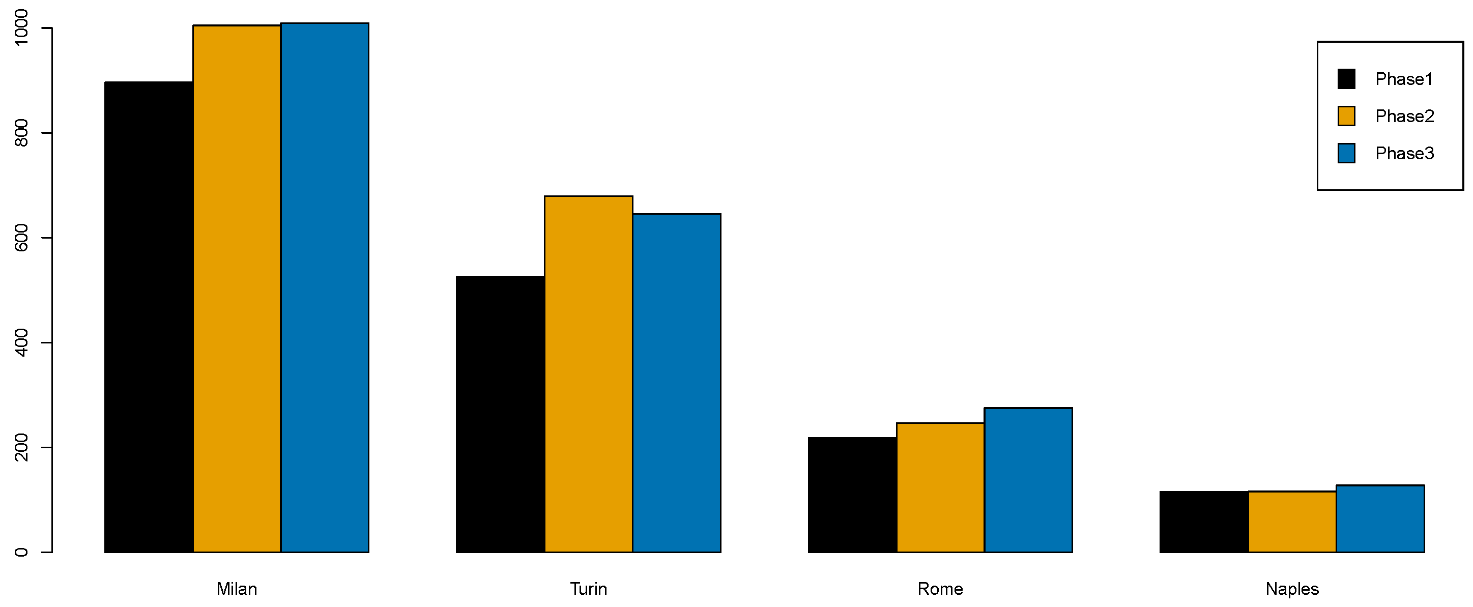
To get a closer look, we report the specific estimated risk of the most affected provinces in the three macro-regions (also the most populated ones) in Figure 5.
The overall risk increases among these provinces, although the strict lockdown action is the most effective restriction in limiting the spatial spread of contagion. Specifically, the provinces that witnessed the higher risk for each macro-region remain the same over time, indicating that some further missing information needs to describe the spatial displacement and the risk spread better.
5. Conclusions
This paper investigated the spread pattern of the COVID-19 in Italy by proposing a spatio-temporal model. We studied and interpreted the evolution of the spread among the 107 Italian provinces. Moreover, the different phases of the COVID-19 history, identified by the Italian government, that are proxies of the citizens’ mobility patterns are considered.
At this aim, we fitted a Besag–York–Mollié model to the disease count data of the COVID-19, spread out the provinces of Italy. Indeed, since the available infection data are counts per spatial unit, the BYM-type model seems appropriate for their description. Furthermore, the BYM model can deal with the description of the spatial neighborhood structure. Since the hierarchical structure of the considered models, the BYM is also computational challenging, using the advantages of the INLA approach for inference. In detail, we first provided the spatial distribution of infections, occurred after the lockdown action in the North of Italy.
Furthermore, by comparing different specifications of the spatio-temporal interaction, we draw some conclusions also about the temporal spread pattern of the disease in the whole Italian territory. Based on the selected spatio-temporal model, both the spatial and temporal random effects are significant. In addition, the interaction between the structured temporal component and the unstructured spatial one is also significant.
Therefore, the results of the proposed analyses are as follows:
- During the pre-lockdown period, the spread of the COVID-19 in the provinces under study could be ascribable to the spatial arrangement of provinces, the same conclusion can not be drawn for the post-lockdown period, since the decreasing number of people moving among provinces;
- The selected spatio-temporal model suggests that the temporal evolution of cases that occurred in each province is independent of the temporal evolution of the other provinces. This means that the number of contagions and their temporal trends may not be caused by the spatial movements of people, but by some aspects that are specific of the considered provinces. That is, for a better comprehension of this spreading phenomenon, point process, even accounting for external information, would be more appropriate;
- The proposed models are our best option for dealing with aggregated data at the district level. Indeed, starting from this low-detailed scale dataset and the absence of geocoded health data, our study still shows the proposed BYM models’ advantages;
- The estimated posterior means of the district-specific relative risk identified the highest-risk areas, confirming that the most at-risk provinces are in Lombardy (i.e., Milan, Bergamo and Brescia) and Piedmont (Turin).
As a general conclusion, our analysis aimed at describing the spread of the infections of COVID-19 cases, and we have not included risk factors or covariates deliberately. However, with the beginning of the so called “second wave” of contagions, it has been established as a known fact that, due to the peculiar infectiousness of this disease, a large portion of the actual infected individuals are asymptomatic. The percentage of asymptomatic individuals can, of course, vary in space and also in time. In any case, these subjects are usually recorded, and, therefore, they are not counted in national databases nor are let alone considered in the available studies. This issue is a further limitation of the known analyses that do not account for the main cases inducing the spread of the COVID-19 disease in space and time. For instance, one could wonder how the population shifting affected the spatial pattern of COVID-19 in Italy. As future work, this could be investigated by means of the inclusion of such information both in the construction of the neighboring scheme, and in the linear predictor as covariates.
Author Contributions
Conceptualization, G.A., A.A. and N.D.; methodology, N.D.; software, N.D.; validation, A.A. and G.A.; formal analysis, G.A., A.A. and N.D.; investigation, N.D.; writing—review and editing, G.A., A.A. and N.D.; supervision, G.A. and A.A. All authors have read and agreed to the published version of the manuscript.
Funding
This research received no external funding.
Data Availability Statement
Italian COVID-19 data supporting reported results can be found at /https://github.com/pcm-dpc/COVID-19 in October 2021. Data are downloaded at the time of writing: October 2020.
Conflicts of Interest
The authors declare no conflict of interest.
References
- Guliyev, H. Determining the spatial effects of COVID-19 using the spatial panel data model. Spat. Stat. 2020, 38, 100443. [Google Scholar] [CrossRef]
- Mollalo, A.; Vahedi, B.; Rivera, K.M. GIS-based spatial modeling of COVID-19 incidence rate in the continental United States. Sci. Total Environ. 2020, 728, 138884. [Google Scholar] [CrossRef] [PubMed]
- Arauzo-Carod, J.M. A first insight about spatial dimension of COVID-19: Analysis at municipality level. J. Public Health 2021, 43, 98–106. [Google Scholar] [CrossRef] [PubMed]
- Cordes, J.; Castro, M.C. Spatial analysis of COVID-19 clusters and contextual factors in New York City. Spat. Spatio-Temporal Epidemiol. 2020, 34, 100355. [Google Scholar] [CrossRef] [PubMed]
- Desjardins, M.; Hohl, A.; Delmelle, E. Rapid surveillance of COVID-19 in the United States using a prospective space-time scan statistic: Detecting and evaluating emerging clusters. Appl. Geogr. 2020, 118, 102202. [Google Scholar] [CrossRef] [PubMed]
- Hohl, A.; Delmelle, E.M.; Desjardins, M.R.; Lan, Y. Daily surveillance of COVID-19 using the prospective space-time scan statistic in the United States. Spat. Spatio-Temporal Epidemiol. 2020, 34, 100354. [Google Scholar] [CrossRef] [PubMed]
- Kang, D.; Choi, H.; Kim, J.H.; Choi, J. Spatial epidemic dynamics of the COVID-19 outbreak in China. Int. J. Infect. Dis. 2020, 94, 96–102. [Google Scholar] [CrossRef] [PubMed]
- Liao, H.; Marley, G.; Si, Y.; Wang, Z.; Xie, Y.; Wang, C.; Tang, W. A Tempo-geographic Analysis of Global COVID-19 Epidemic Outside of China. medRxiv 2020. [Google Scholar] [CrossRef]
- Ramírez-Aldana, R.; Gomez-Verjan, J.C.; Bello-Chavolla, O.Y. Spatial analysis of COVID-19 spread in Iran: Insights into geographical and structural transmission determinants at a province level. PLoS Neglected Trop. Dis. 2020, 14, e0008875. [Google Scholar] [CrossRef]
- Chen, Y.C.; Lu, P.E.; Chang, C.S.; Liu, T.H. A Time-Dependent SIR Model for COVID-19 With Undetectable Infected Persons. IEEE Trans. Netw. Sci. Eng. 2020, 7, 3279–3294. [Google Scholar] [CrossRef]
- Giordano, G.; Blanchini, F.; Bruno, R.; Colaneri, P.; Di Filippo, A.; Di Matteo, A.; Colaneri, M. Modelling the COVID-19 epidemic and implementation of population-wide interventions in Italy. Nat. Med. 2020, 26, 855–860. [Google Scholar] [CrossRef]
- Gatto, M.; Bertuzzo, E.; Mari, L.; Miccoli, S.; Carraro, L.; Casagrandi, R.; Rinaldo, A. Spread and dynamics of the COVID-19 epidemic in Italy: Effects of emergency containment measures. Proc. Natl. Acad. Sci. USA 2020, 117, 10484–10491. [Google Scholar] [CrossRef] [PubMed] [Green Version]
- Dehning, J.; Zierenberg, J.; Spitzner, F.P.; Wibral, M.; Neto, J.P.; Wilczek, M.; Priesemann, V. Inferring change points in the spread of COVID-19 reveals the effectiveness of interventions. Science 2020, 369, eabb9789. [Google Scholar] [CrossRef]
- Ioannidis, J.P.; Cripps, S.; Tanner, M.A. Forecasting for COVID-19 has failed. Int. J. Forecast. 2020. [Google Scholar] [CrossRef] [PubMed]
- D’Angelo, N.; Adelfio, G.; Abbruzzo, A. Spatio-temporal analysis of the Covid-19 spread in Italy by Bayesian hierarchical models. In Book of Short Papers—SIS 2021; Pearson: New York, NY, USA, 2021; pp. 1016–1020. [Google Scholar]
- Wu, X.; Nethery, R.C.; Sabath, M.B.; Braun, D.; Dominici, F. Air pollution and COVID-19 mortality in the United States: Strengths and limitations of an ecological regression analysis. Sci. Adv. 2020, 6, eabd4049. [Google Scholar] [CrossRef] [PubMed]
- Besag, J.; York, J.; Mollié, A. Bayesian image restoration, with two applications in spatial statistics. Ann. Inst. Stat. Math. 1991, 43, 1–20. [Google Scholar] [CrossRef]
- Abellan, J.J.; Richardson, S.; Best, N. Use of space–time models to investigate the stability of patterns of disease. Environ. Health Perspect. 2008, 116, 1111–1119. [Google Scholar] [CrossRef] [PubMed] [Green Version]
- Lawson, A.B. Bayesian Disease Mapping: Hierarchical Modeling in Spatial Epidemiology; CRC Press: Boca Raton, FL, USA, 2013. [Google Scholar]
- Møller, J.; Syversveen, A.R.; Waagepetersen, R.P. Log gaussian cox processes. Scand. J. Stat. 1998, 25, 451–482. [Google Scholar] [CrossRef]
- Konstantinoudis, G.; Schuhmacher, D.; Rue, H.; Spycher, B.D. Discrete versus continuous domain models for disease mapping. Spat. Spatio-Temporal Epidemiol. 2020, 32, 100319. [Google Scholar] [CrossRef] [PubMed]
- Li, Y.; Brown, P.; Gesink, D.C.; Rue, H. Log Gaussian Cox processes and spatially aggregated disease incidence data. Stat. Methods Med. Res. 2012, 21, 479–507. [Google Scholar] [CrossRef]
- Loro, P.A.D.; Divino, F.; Farcomeni, A.; Lasinio, G.J.; Lovison, G.; Maruotti, A.; Mingione, M. Nowcasting COVID-19 incidence indicators during the Italian first outbreak. arXiv 2020, arXiv:2010.12679. [Google Scholar]
- Briz-Redón, Á. The impact of modelling choices on modelling outcomes: A spatio-temporal study of the association between COVID-19 spread and environmental conditions in Catalonia (Spain). Stoch. Environ. Res. Risk Assess. 2021, 1–13. [Google Scholar] [CrossRef]
- Elliot, P.; Wakefield, J.C.; Best, N.G.; Briggs, D.J. Spatial Epidemiology: Methods and Applications; Oxford University Press: Oxford, UK, 2000. [Google Scholar]
- Lesaffre, E.; Lawson, A.B. Bayesian Biostatistics; John Wiley & Sons: Hoboken, NJ, USA, 2012. [Google Scholar]
- Tiefelsdorf, M.; Griffith, D.A.; Boots, B. A variance-stabilizing coding scheme for spatial link matrices. Environ. Plan. A 1999, 31, 165–180. [Google Scholar] [CrossRef]
- Kelejian, H.H.; Prucha, I.R. Specification and estimation of spatial autoregressive models with autoregressive and heteroskedastic disturbances. J. Econom. 2010, 157, 53–67. [Google Scholar] [CrossRef] [PubMed] [Green Version]
- Sørbye, S.H.; Rue, H. Scaling intrinsic Gaussian Markov random field priors in spatial modelling. Spat. Stat. 2014, 8, 39–51. [Google Scholar] [CrossRef]
- MacNab, Y.C. On Gaussian Markov random fields and Bayesian disease mapping. Stat. Methods Med. Res. 2011, 20, 49–68. [Google Scholar] [CrossRef]
- Riebler, A.; Sørbye, S.H.; Simpson, D.; Rue, H. An intuitive Bayesian spatial model for disease mapping that accounts for scaling. Stat. Methods Med. Res. 2016, 25, 1145–1165. [Google Scholar] [CrossRef] [Green Version]
- Dean, C.; Ugarte, M.; Militino, A. Detecting interaction between random region and fixed age effects in disease mapping. Biometrics 2001, 57, 197–202. [Google Scholar] [CrossRef] [PubMed]
- Simpson, D.; Rue, H.; Riebler, A.; Martins, T.G.; Sørbye, S.H. Penalising model component complexity: A principled, practical approach to constructing priors. Stat. Sci. 2017, 32, 1–28. [Google Scholar] [CrossRef]
- Moraga, P. Geospatial Health Data: Modeling and Visualization with R-INLA and Shiny; CRC Press: Boca Raton, FL, USA, 2019. [Google Scholar]
- Best, N.; Richardson, S.; Thomson, A. A comparison of Bayesian spatial models for disease mapping. Stat. Methods Med. Res. 2005, 14, 35–59. [Google Scholar] [CrossRef]
- Anderson, C.; Lee, D.; Dean, N. Bayesian cluster detection via adjacency modelling. Spat. Spatio-Temporal Epidemiol. 2016, 16, 11–20. [Google Scholar] [CrossRef] [Green Version]
- Bernardinelli, L.; Clayton, D.; Pascutto, C.; Montomoli, C.; Ghislandi, M.; Songini, M. Bayesian analysis of space—Time variation in disease risk. Stat. Med. 1995, 14, 2433–2443. [Google Scholar] [CrossRef]
- Knorr-Held, L. Bayesian modelling of inseparable space-time variation in disease risk. Stat. Med. 2000, 19, 2555–2567. [Google Scholar] [CrossRef] [Green Version]
- Clayton, D.G. Generalized linear mixed models. Markov Chain Monte Carlo Pract. 1996, 1, 275–302. [Google Scholar]
- Blangiardo, M.; Cameletti, M. Spatial and Spatio-Temporal Bayesian Models with R-INLA; John Wiley-Sons: Hoboken, NJ, USA, 2015. [Google Scholar]
- Goicoa, T.; Adin, A.; Ugarte, M.; Hodges, J. In spatio-temporal disease mapping models, identifiability constraints affect PQL and INLA results. Stoch. Environ. Res. Risk Assess. 2018, 32, 749–770. [Google Scholar] [CrossRef]
- Gelfand, A.E.; Diggle, P.; Guttorp, P.; Fuentes, M. Handbook of Spatial Statistics; CRC Press: Boca Raton, FL, USA, 2010. [Google Scholar]
- Allard, D. Handbook of Spatial Statistics. Book Review; Gelfand, A.E., Diggle, P.J., Fuentes, M., Peter Guttorp, Eds.; CRC Press: Boca Raton, FL, USA, 2011; Volume 21, pp. 293–294. [Google Scholar]
- Hastings, W.K. Monte Carlo sampling methods using Markov chains and their applications. Biometrika 1970, 57, 97–109. [Google Scholar] [CrossRef]
- Rue, H.; Martino, S.; Chopin, N. Approximate Bayesian inference for latent Gaussian models by using integrated nested Laplace approximations. J. R. Stat. Soc. Ser. B Stat. Methodol. 2009, 71, 319–392. [Google Scholar] [CrossRef]
- Martins, T.G.; Simpson, D.; Lindgren, F.; Rue, H. Bayesian computing with INLA: New features. Comput. Stat. Data Anal. 2013, 67, 68–83. [Google Scholar] [CrossRef] [Green Version]
- Blangiardo, M.; Cameletti, M.; Baio, G.; Rue, H. Spatial and spatio-temporal models with R-INLA. Spat. Spatio-Temporal Epidemiol. 2013, 4, 33–49. [Google Scholar] [CrossRef] [PubMed] [Green Version]
- Lindgren, F.; Rue, H.; Lindström, J. An explicit link between Gaussian fields and Gaussian Markov random fields: The stochastic partial differential equation approach. J. R. Stat. Soc. Ser. B Stat. Methodol. 2011, 73, 423–498. [Google Scholar] [CrossRef] [Green Version]
- Bisanzio, D.; Giacobini, M.; Bertolotti, L.; Mosca, A.; Balbo, L.; Kitron, U.; Vazquez-Prokopec, G.M. Spatio-temporal patterns of distribution of West Nile virus vectors in eastern Piedmont Region, Italy. Parasites Vectors 2011, 4, 230. [Google Scholar] [CrossRef] [PubMed] [Green Version]
- Schrödle, B.; Held, L. Spatio-temporal disease mapping using INLA. Environmetrics 2011, 22, 725–734. [Google Scholar] [CrossRef]
- Schrödle, B.; Held, L.; Rue, H. Assessing the Impact of a Movement Network on the Spatiotemporal Spread of Infectious Diseases. Biometrics 2012, 68, 736–744. [Google Scholar] [CrossRef]
- Cameletti, M.; Lindgren, F.; Simpson, D.; Rue, H. Spatio-temporal modeling of particulate matter concentration through the SPDE approach. AStA Adv. Stat. Anal. 2013, 97, 109–131. [Google Scholar] [CrossRef] [Green Version]
- Gómez-Rubio, V.; Bivand, R.; Rue, H. A New Latent Class to Fit Spatial Econometrics Models with Integrated Nested Laplace Approximations. Procedia Environ. Sci. 2015, 27, 116–118. [Google Scholar] [CrossRef] [Green Version]
- R Core Team. R: A Language and Environment for Statistical Computing; R Foundation for Statistical Computing: Vienna, Austria, 2019. [Google Scholar]
- Adin, A.; Goicoa, T.; Ugarte, M.D. Online relative risks/rates estimation in spatial and spatio-temporal disease mapping. Comput. Methods Programs Biomed. 2019, 172, 103–116. [Google Scholar] [CrossRef] [Green Version]
- Haug, N.; Geyrhofer, L.; Londei, A.; Dervic, E.; Desvars-Larrive, A.; Loreto, V.; Pinior, B.; Thurner, S.; Klimek, P. Ranking the effectiveness of worldwide COVID-19 government interventions. Nat. Hum. Behav. 2020, 4, 1303–1312. [Google Scholar] [CrossRef]
- Richardson, S.; Thomson, A.; Best, N.; Elliott, P. Interpreting posterior relative risk estimates in disease-mapping studies. Environ. Health Perspect. 2004, 112, 1016–1025. [Google Scholar] [CrossRef]
- Meyer, S.; Held, L.; Höhle, M. Spatio-temporal analysis of epidemic phenomena using the R package surveillance. arXiv 2014, arXiv:1411.0416. [Google Scholar] [CrossRef] [Green Version]
- Adelfio, G.; Chiodi, M. Including covariates in a space-time point process with application to seismicity. Stat. Methods Appl. 2021, 30, 947–971. [Google Scholar] [CrossRef]
Figure 1.
Total number of cases recorded per province corrected by 1000 inhabitants. Top panel: Pre-lockdown period. Bottom panel: Post-lockdown period.
Figure 1.
Total number of cases recorded per province corrected by 1000 inhabitants. Top panel: Pre-lockdown period. Bottom panel: Post-lockdown period.

Figure 2.
Detecting cases relative risk specific of the province in the disease mapping models. Left panel: pre-lockdown model. Right panel: post-lockdown model.
Figure 2.
Detecting cases relative risk specific of the province in the disease mapping models. Left panel: pre-lockdown model. Right panel: post-lockdown model.
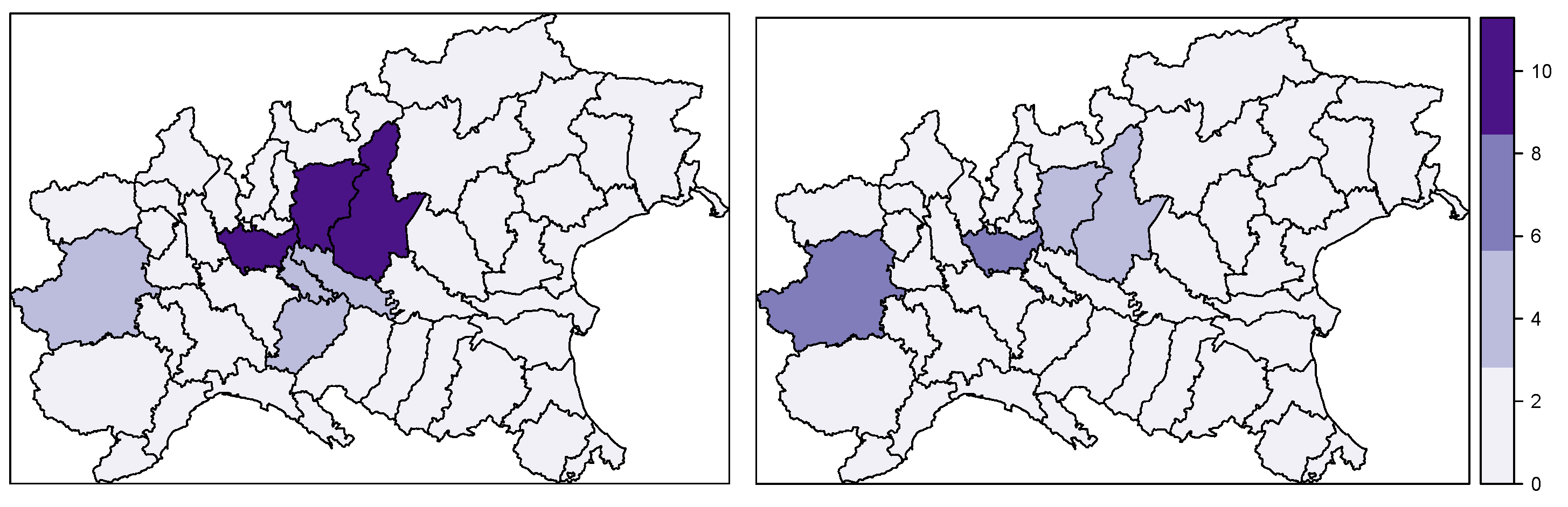
Figure 3.
Daily new cases in Italy during the first wave of infections. The vertical blue straight lines individuate the three phases.
Figure 3.
Daily new cases in Italy during the first wave of infections. The vertical blue straight lines individuate the three phases.
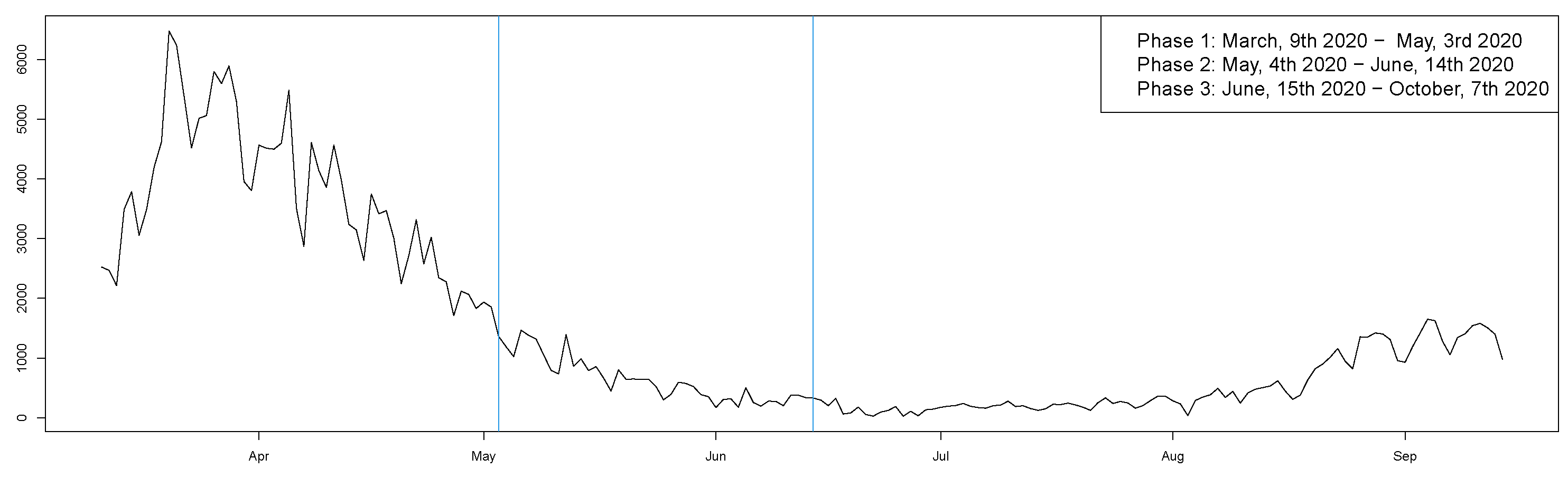
Figure 4.
Province-specific relative risks of COVID-19 cases in Italy under the chosen model (temporally structured interaction) by macro-region for the three phases considered.
Figure 4.
Province-specific relative risks of COVID-19 cases in Italy under the chosen model (temporally structured interaction) by macro-region for the three phases considered.

Figure 5.
Top province-specific estimated risk for the three macro-regions.

Table 1.
DIC values for the spatial and spatio-temporal fitted models.
| Model | Interactions | Spatial Correlation | Temporal Correlation | DIC |
|---|---|---|---|---|
| BYM | – | – | – | 135,642.433 |
| Linear T | – | – | – | 52,002.912 |
| Type I | and | – | – | 4695.569 |
| Type II | and | – | ✓ | 4695.264 |
| Type III | and | ✓ | – | 4695.281 |
| Type IV | and | ✓ | ✓ | 5441.607 |
Publisher’s Note: MDPI stays neutral with regard to jurisdictional claims in published maps and institutional affiliations. |
© 2021 by the authors. Licensee MDPI, Basel, Switzerland. This article is an open access article distributed under the terms and conditions of the Creative Commons Attribution (CC BY) license (https://creativecommons.org/licenses/by/4.0/).
Share and Cite
MDPI and ACS Style
D’Angelo, N.; Abbruzzo, A.; Adelfio, G. Spatio-Temporal Spread Pattern of COVID-19 in Italy. Mathematics 2021, 9, 2454. https://doi.org/10.3390/math9192454
AMA Style
D’Angelo N, Abbruzzo A, Adelfio G. Spatio-Temporal Spread Pattern of COVID-19 in Italy. Mathematics. 2021; 9(19):2454. https://doi.org/10.3390/math9192454
Chicago/Turabian StyleD’Angelo, Nicoletta, Antonino Abbruzzo, and Giada Adelfio. 2021. "Spatio-Temporal Spread Pattern of COVID-19 in Italy" Mathematics 9, no. 19: 2454. https://doi.org/10.3390/math9192454
Note that from the first issue of 2016, this journal uses article numbers instead of page numbers. See further details here.