Distribution Linguistic Fuzzy Group Decision Making Based on Consistency and Consensus Analysis

Abstract

The development of distribution linguistic provides a new research idea for linguistic information group decision-making (GDM) problems, which is more flexible and convenient for experts to express their opinions. However, in the process of using distribution linguistic fuzzy preference relations (DLFPRs) to solve linguistic information GDM problems, there are few studies that pay attention to both internal consistency adjustment and external consensus of experts. Therefore, this study proposes a fresh decision support model based on consistency adjustment algorithm and consensus adjustment algorithm to solve GDM problems with distribution linguistic data. Firstly, we review the concept of DLFPRs to describe the fuzzy linguistic evaluation information, and then we present the multiplicative consistency of DLFPRs and a new consistency measurement method based on the distance, and investigate the consistency adjustment algorithm to ameliorate the consistency level of DLFPRs. Subsequently, the consensus degree measurement is carried out, and a new consensus degree calculation method is put forward. At the same time, the consensus degree adjustment is taken the expert cost into account to make it reach the predetermined level. Finally, a distribution linguistic fuzzy group decision making (DLFGDM) method is designed to integrate the evaluation linguistic elements and obtain the final evaluation information. A case of the evaluation of China’s state-owned enterprise equity incentive model is provided, and the validity and superiority of the proposed method are performed by comparative analysis.

1. Introduction

GDM is an overall process where many people take part in decision-making analysis and make decisions aiming to make the best of the collective wisdom. Decision-making method is also widely used, such as public transportation development decision [1], passenger satisfaction evaluation [2], equity incentive decision-making [3], etc. Particularly, with economic development, equity incentive plays an increasingly important role in the development of enterprises. Wang et al. [3] used rough set theory as research method to study the influencing factors of equity incentive mode decision-making of listed companies. However, there are few researches on equity incentive methods in GDM problems, so we also turn the research and application direction of this paper to this field.

Due to subjective and objective reasons, including the complicacy and fuzziness of decision-making scenes and the limited knowledge of experts, we cannot express evaluation information by clear values. In this case, fuzzy preference relation (FRL) [4] appeared to flexibly express pairwise comparison evaluation. FRL was extended into hesitant fuzzy preference relation [5], Pythagorean fuzzy preference relation [6], which are all preference relations based on numbers. At the same time, because the traditional GDM is not very effective in dealing with the fuzziness of evaluation, the fuzzy group decision making method is also widely used [7]. Wu et al. [7] proposed a fuzzy group decision model, which is on the foundation of a new compatibility measure with multiplicative trapezoidal fuzzy preference relations.

However, the environment is complex and not all problems can be evaluated numerically. Therefore, Zadeh [8] studied the fuzzy linguistic method and derived the linguistic preference relation (LPR). LPR can express the evaluation information by using the linguistic variable in the linguistic term sets [9], which is more consistent with the human thinking inertia. Furthermore, Zhang et al. [10] utilized the linguistic distribution term sets (LDTSs) and put forward the distribution linguistic fuzzy preference relations (DLFPRs) to represent the evaluation information, which can utilize different linguistic vocabulary in different degrees. For example, when experts are invited to evaluate several equity incentive methods, he/she has a tendency of 30% to choose “very good”, a tendency of 60% to choose “good”, a tendency of 10% to choose “medium”. DLFPR is a great development of LPR and plays a great role in decision making. Many researches in this field have made some achievements.

Guo et al. [11] proposed a proportional fuzzy linguistic distribution model to deal with incomplete linguistic evaluation. Huang et al. [12] developed linguistic distribution assessment to represent rick assessment information and combined it with an improved TODIM method for analysis. Based on linguistic distribution and the application of hesitant fuzzy linguistic term sets, Wu et al. [13] proposed a new linguistic decision model and called it maximum support decision model. Liang et al. [14] and Ju et al. [15] conducted an in-depth study on multi-granularity language distribution evaluation and put it into application. Wang et al. [16] explored the unbalanced environment of linguistic distribution evaluation, extended the comparison method, distance measurement and other related contents, and proposed an asymmetric trapezoidal cloud-based linguistic group decision-making model.

From the research results of GDM using DLFPRs, consistency checking and improvement is an important process. Thus, so far, there has been some progress on consistency. Dong et al. [17,18] and Jin et al. [19,20] gave the consistency definition of fuzzy linguistic preference relations and Zhang et al. [10] gave the consistency definition of DLFPRs. Tang et al. [21] studied the personalized linguistic term environment, analyzed the properties of additive consistency and multiplicative consistency of DLFPRs, then constructed a new consistency driven optimization model. Zhao et al. [22] and Wang et al. [23] explored the decision-making situation of incomplete linguistic preference relation, established target model and estimated the missing value of preference relation. In establishing consistency algorithm, Zhao et al. [22] proposed a multi-stage algorithm that considered and adjusted individual consistency and group consistency. Wang et al. [23] defined a weak consistency algorithm to interact with experts, flexibly solicit expert opinions, and then complement with additive consistency. When different experts have different degrees of uncertainty, it is necessary to study the consistency of multi-granularity context. Cai et al. [24] established a consistency index based on the distance of multi-granularity language preference relationship, and used Chi-square statistics as the consistency threshold. Zhao et al. [25] proposed a sufficient condition to describe the multi-granularity aggregation mechanism of consistency and used an attitudinal language approach to improve consistency ranking. With the development of society, consistency recognition and improvement have been put into use in all kinds of fields, such as investment decision-making [26,27], public health emergency decision making [28], stock selection decision-making [29], etc.

However, owing to decision makers (DMs) have different knowledge background and personal preference, there may be differences between them, thus, consensus is also an important part of decision-making. Zhang et al. [30] explored a new consensus-oriented aggregation model for GDM, making use of the maximum consensus to form collective opinion, and then combined the lowest consensus cost model to propose the entire consensus-reaching process. Liu et al. [31] proffered a new maximum consensus model to measure similarity from two dimensions of direction and module, which is more convenient for application. In the research of consensus reaching in multi-attribute group decision making (MAGDM) [32,33,34,35,36], Yao [32] used (MAGDM) represented by linguistic distribution evaluation as the background. It identified experts based on recognition rules and adjusted their preferences according to the optimization model, minimizing the discrepancy between the output value and the initial value, and preserving the initial evaluation information as much as possible, making it completer and more reliable. Yu et al. [36] defined the group consensus degree based on multi-granular hesitant fuzzy linguistic terms, combined with the optimization model of minimum adjustment, designed an iterative algorithm to help DMs reach consensus in MAGDM. Wu et al. [37] proposed a new indicator and consensus evolution networks to measure the consensus degree and reflect the evolution of consensus more clearly.

Combined with the above research results and analysis, we can know that using DLFPRs to solve fuzzy and complex GDM problems has become an effective research direction. Although many achievements have been made in this field, some shortcomings remain to be developed. Therefore, this paper continues to study this aspect and uses DLFPR to express expert evaluation information. At the same time, this paper uses the recognition and adjustment mechanism of consistency level and consensus degree to reach the internal and external consensus of experts, so that we can make the most reasonable and reliable decision-making, which can make up for the deficiencies of the current research. Zhang et al. [10] introduced the concept of DLFPR, studied the operation rules of language distribution estimation, defined the multiplicative consistency and additive consistency of preference relation of distributed language, and gave their ideal properties. In addition, a new consensus model including recognition rules and adjustment rules was proposed. The recognition rules are based on matrix distance and arithmetic average operator, which needs to be improved. On the basis of using different types of numerical scale, Tang et al. [38] related DLFPRs with FRL and multiplicative preference relation, defined the expectation consistency of DLFPRs, proposed some goal programming models, derived personalized numerical scale of language terms, which can fill the research defect of personalized semantics. However, Tang et al. [38] only considered the consistency within the experts and did not consider the differences caused by the different cultural and knowledge backgrounds among the experts, so there was no consensus among the experts.

According to the above analysis, there are still few researches on DLFPRs and some defects. Therefore, it is of great significance to study the consistency adjustment process and consensus reaching process of DLFPRs. This paper mainly uses the empirical research method, using mathematical empirical research and case empirical research, to study and prove the theoretical hypothesis, and then puts forward some algorithms to optimize the process, and finally applies it to the case to verify its feasibility. The key contributions of this article are listed as follows:

• The consistency of DLFPRs is redefined, and only the probability variation is considered, so the calculation is easier to understand.
• A new iterative algorithm for consistency recognition and adjustment is proposed to improve consistency level to acceptable level.
• A new iterative algorithm for recognition and adjustment of group consensus degree is proposed to improve group consensus degree.

The residue part of the article is formulated as follows. Section 2 introduces the basic concept of LDTSs, DLFPRs. Section 3 redeclares the multiplication consistency of DLFPRs and a new consistency recognition and adjustment algorithm is proposed. Section 4 designs a new algorithm for group consensus recognition and adjustment, including the consideration of expert cost. In Section 5, the developed DLFGDM model is established including consistency adjustment process, consensus reaching process, information integration, ideal scheme selection. In Section 6, by giving numerical examples of equity incentive mode selection, the method developed in this paper is in comparison with other methods to analyze and appraise the actual utility and advantages of it. In Section 7, we draw the conclusion of this article and indicate the future research direction.

2. Preliminaries

In this part, we briefly retrospect the LDTSs and outline the concept of DLFPRs.

2.1. Linguistic Distribution Term Sets (LDTSs)

A fuzzy linguistic distribution term set is indicated as $S=\left\{s_{\xi }|\xi =0,1,\dots ,2\tau \right\}$ with odd cardinality, where the number of $s_{\xi }$ is known as the cardinality of $S$ [8,39,40,41,42,43,44,45].

It is necessitated that the fuzzy LDTSs ought to fulfill the characteristics as follows:

• If $s_{\xi }\le s_{\psi }$, then $\xi \le \psi$;
• If $\xi =2\tau -\psi$, then $neg(s_{\xi })=s_{\psi }$, especially $s_{\tau }=neg(s_{\tau })$.

Example 1.

To assess the size of a coffee cup, experts can express their inclinations by utilizing the following LTDS:

$$S=\left\{s_0:very small, s_1:small, s_2:medium, s_3:big, s_4:very big\right\}$$

2.2. Distribution Linguistic Fuzzy Preference Relations (DLFPRs)

When making pairwise comparisons in decision making, it is beneficial to express their preference over elections. In this case, the DMs can utilize assessments of the linguistic term set mentioned above. Thus, the concept of DLFPRs is introduced.

Definition 1.

Supposing that $X=\left\{x_1,x_2,\dots ,x_n\right\}$ is an alternative set, $S=\left\{s_{\xi }|\xi =0,1,\dots ,2\tau \right\}$ is a LDTS, and a DLFPR on $X$ is defined as $H\subset X\times X$, $H={(h_{ij})}_{n\times n}$ with a distribution linguistic fuzzy element (DLFE) $h_{ij}=\left\{(s_{\xi },p_{ij}^{(\xi )})|\xi =0,1,\dots ,2\tau ,0\le p_{ij}^{(\xi )}\le 1,{\displaystyle \sum _{\xi =0}^{2\tau }{p}_{ij}^{(\xi )}=1}\right\}$, which is referred to as a linguistic distribution preference of $S$, where $p_{ij}^{(\xi )}$ represents the corresponding probability of $s_{\xi }$ in the relation between $x_i$ and $x_j$. In addition, the following conditions are satisfied by $(s_{\xi },p_{ij}^{(\xi )})$:

• $p_{ij}^{(\xi )}=p_{jl}^{(2\tau -\xi )},\forall i,j=1,2,\dots ,n,\xi =0,1,\dots ,2\tau$;
• $h_{ii}=\left\{(s_{\tau },1)\right\}$.

3. Consistency-Adjustment Algorithm for DLFPRs

In view of the uncertainty of the item itself and the influence of subjective and objective factors such as the structure of expert knowledge, experts’ evaluation of decision may have strong of personal color, which is hard to supply DLFPRs with perfect consistency. Hence, it is essential to improve DLFPRs.

The section contains three parts. First, characterize the concept of the multiplicative consistency of DLFPRs. Then, construct a consistency index for DLFPRs to quantify the consistency level of DLFPRs. Based on them, we propose a method for developing the consistency level.

3.1. Multiplicative Consistency of DLFPRs

To develop the theory based on the multiplicative consistency of FRL, the multiplicative consistency of DLFPRs is described as below:

Definition 2.

Let $H={(h_{ij})}_{n\times n}$ be a DLFPR, where $h_{ij}=\{(s_{\xi },p_{ij}^{(\xi )})|\xi =0,1,\dots ,2\tau , 0\le p_{ij}^{(\xi )}\le 1, {\displaystyle \sum _{\xi =0}^{2\tau }{p}_{ij}^{(\xi )}=1}\}$. If $H={(h_{ij})}_{n\times n}$ satisfies the following conditions:

$$\forall i,j,l=1,2,\dots ,n, \xi =0,1,\dots ,2\tau , p_{ij}^{(\xi )}{p}_{jl}^{(\xi )}{p}_{li}^{(\xi )}=p_{il}^{(\xi )}{p}_{lj}^{(\xi )}{p}_{ji}^{(\xi )},$$

(1)

then $H={(h_{ij})}_{n\times n}$ is a DLFPR with multiplicative consistency.

Remark 1.

In [21,46], there has been some development in the consistency of DLFPRs, but it still has some drawbacks such as complexity of calculation. Thus, we redefine multiplicative consistency as follows.

Theorem 1.

Given a DLFPR $H={(h_{ij})}_{n\times n}$, where $h_{ij}=\{(s_{\xi },p_{ij}^{(\xi )})|\xi =0,1,\dots ,2\tau ,0\le p_{ij}^{(\xi )}\le 1$, ${\displaystyle \sum _{\xi =0}^{2\tau }{p}_{ij}^{(\xi )}=1}\}$, then $\tilde{H}={({\tilde{h}}_{ij})}_{n\times n}$ is a DLFPR with multiplicative consistency, where ${\tilde{h}}_{ij}=\left\{{(\mathrm{s}}_{\xi },{\tilde{p}}_{ij}^{(\xi )})|\xi =0,1,\dots ,2\tau ,0\le {\tilde{p}}_{ij}^{(\xi )}\le 1,{\displaystyle \sum _{\xi =0}^{2\tau }{\tilde{p}}_{ij}^{(\xi )}=1}\right\}$ and ${\tilde{p}}_{ij}^{(\xi )}=\{\begin{array}{l}{\widehat{p}}_{ij}^{(\xi )}/{\displaystyle \sum _{\xi =0}^{2\tau }{\widehat{p}}_{ij}^{(\xi )}},i<j\\ p_{ij}^{(\xi )},\hspace{1em}\hspace{1em}\hspace{1em} i=j\\ {\tilde{p}}_{ji}^{(2\tau -\xi )},\hspace{1em}\hspace{1em}i>j\end{array}$, where

$${\widehat{p}}_{ij}^{(\xi )}={\left(1+\frac{{\displaystyle \sum _{l=1}^n{p}_{jl}^{(\xi )}}}{{\displaystyle \sum _{l=1}^n{p}_{il}^{(\xi )}}}\right)}^{-1},$$

(2)

satisfies the following:

(1) 

$0\le {\tilde{p}}_{ij}^{(\xi )}\le 1$;

(2) 

$\tilde{H}$ is DLFPR;

(3) 

$p_{ij}^{(\xi )}{p}_{jl}^{(\xi )}{p}_{li}^{(\xi )}=p_{il}^{(\xi )}{p}_{lj}^{(\xi )}{p}_{ji}^{(\xi )}$.

Proof of Theorem 1.

(1)

For $\forall i,j,l=1,2,\dots ,n$, $0\le p_{ij}^{(\xi )}\le 1$, we have: $0\le p_{il}^{(\xi )}\le 1$, $0\le p_{jl}^{(\xi )}\le 1$, then $\frac{{\displaystyle \sum _{l=1}^n{p}_{jl}^{(\xi )}}}{{\displaystyle \sum _{l=1}^n{p}_{il}^{(\xi )}}}>0$. Thus,

$$0\le {\tilde{p}}_{ij}^{(\xi )}={\left(1+\frac{{\displaystyle \sum _{l=1}^n{p}_{jl}^{(\xi )}}}{{\displaystyle \sum _{l=1}^n{p}_{il}^{(\xi )}}}\right)}^{-1}/{\displaystyle \sum _{\xi =0}^{2\tau }{\left(1+\frac{{\displaystyle \sum _{l=1}^n{p}_{jl}^{(\xi )}}}{{\displaystyle \sum _{l=1}^n{p}_{il}^{(\xi )}}}\right)}^{-1}}\le 1.$$

(3)

(2)

For $\forall i,j=1,2,\dots ,n$, when $i=j$, ${\tilde{p}}_{ij}^{(\xi )}=p_{ij}^{(\xi )}$, we can obtain ${\tilde{h}}_{ii}=\{(s_0,0),\dots ,(s_{\tau -1},0),(s_{\tau },1),(s_{\tau +1},0),\dots ,(s_{2\tau },0)\}$.

Thus, $\tilde{H}={({\tilde{h}}_{ij})}_{n\times n}$ is a DLFPR.

(3)

For $\forall i,j,l=1,2,\dots ,n,\xi =0,1,\dots ,2\tau$, ${\widehat{p}}_{ij}^{(\xi )}+{\widehat{p}}_{ji}^{(\xi )}=1$, we can attest:

$$\begin{array}{l}\frac{{\widehat{p}}_{il}^{(\xi )}}{{\widehat{p}}_{li}^{(\xi )}}\cdot \frac{{\widehat{p}}_{lj}^{(\xi )}}{{\widehat{p}}_{jl}^{(\xi )}}=\frac{1}{1-{\widehat{p}}_{il}^{(\xi )}}\cdot \frac{1}{1-{\widehat{p}}_{lj}^{(\xi )}}=\frac{1}{1/{\widehat{p}}_{il}^{(\xi )}-1}\cdot \frac{1}{1/{\widehat{p}}_{lj}^{(\xi )}-1}\\ =\frac{1}{{\displaystyle \sum _{l=1}^n{p}_{ll}^{(\xi )}}/{\displaystyle \sum _{l=1}^n{p}_{il}^{(\xi )}}}\cdot \frac{1}{{\displaystyle \sum _{l=1}^n{p}_{jl}^{(\xi )}}/{\displaystyle \sum _{l=1}^n{p}_{ll}^{(\xi )}}}\\ =\frac{{\displaystyle \sum _{l=1}^n{p}_{il}^{(\xi )}}}{{\displaystyle \sum _{l=1}^n{p}_{jl}^{(\xi )}}}=\frac{1+\frac{{\displaystyle \sum _{l=1}^n{p}_{jl}^{(\xi )}}}{{\displaystyle \sum _{l=1}^n{p}_{il}^{(\xi )}}}}{1+\frac{{\displaystyle \sum _{l=1}^n{p}_{il}^{(\xi )}}}{{\displaystyle \sum _{l=1}^n{p}_{jl}^{(\xi )}}}}=\frac{{\left(1+\frac{{\displaystyle \sum _{l=1}^n{p}_{jl}^{(\xi )}}}{{\displaystyle \sum _{l=1}^n{p}_{il}^{(\xi )}}}\right)}^{-1}}{{\left(1+\frac{{\displaystyle \sum _{l=1}^n{p}_{il}^{(\xi )}}}{{\displaystyle \sum _{l=1}^n{p}_{jl}^{(\xi )}}}\right)}^{-1}}=\frac{{\widehat{p}}_{ij}^{(\xi )}}{{\widehat{p}}_{ji}^{(\xi )}},\end{array}$$

(4)

Then,

$$\begin{array}{l}\frac{{\tilde{p}}_{il}^{(\xi )}}{{\tilde{p}}_{li}^{(\xi )}}\cdot \frac{{\tilde{p}}_{jl}^{(\xi )}}{{\tilde{p}}_{lj}^{(\xi )}}=\frac{{\widehat{p}}_{il}^{(\xi )}}{{\displaystyle \sum {\widehat{p}}_{il}^{(\xi )}}}\cdot \frac{{\displaystyle \sum {\widehat{p}}_{li}^{(\xi )}}}{{\widehat{p}}_{li}^{(\xi )}}\cdot \frac{{\widehat{p}}_{lj}^{(\xi )}}{{\displaystyle \sum {\widehat{p}}_{lj}^{(\xi )}}}\cdot \frac{{\displaystyle \sum {\widehat{p}}_{jl}^{(\xi )}}}{{\widehat{p}}_{jl}^{(\xi )}}\\ =\frac{{\widehat{p}}_{ij}^{(\xi )}}{{\widehat{p}}_{ji}^{(\xi )}}\cdot \frac{{\displaystyle \sum {\widehat{p}}_{ji}^{(\xi )}}}{{\displaystyle \sum {\widehat{p}}_{ij}^{(\xi )}}}=\frac{{\tilde{p}}_{ij}^{(\xi )}}{{\tilde{p}}_{ji}^{(\xi )}},\end{array}$$

(5)

Thus, we can obtain:

$$\mathrm{i}.\mathrm{e}., \forall i,j,l=1,2,\dots ,n,\xi =0,1,\dots ,2\tau ,p_{ij}^{(\xi )}{p}_{jl}^{(\xi )}{p}_{li}^{(\xi )}=p_{il}^{(\xi )}{p}_{lj}^{(\xi )}{p}_{ji}^{(\xi )}$$

(6)

Thus, DLFPR $\tilde{H}={({\tilde{h}}_{ij})}_{n\times n}$ is of multiplicative consistency, which finishes the attestation of Theorem 1. □

On the basis of them, we can propose the following one.

Theorem 2.

Given a DLFPR $H={(h_{ij})}_{n\times n}$ with $h_{ij}=\{(s_{\xi },p_{ij}^{(\xi )})|\xi =0,1,\dots ,2\tau ,0\le p_{ij}^{(\xi )}\le 1,{\displaystyle \sum _{\xi =0}^{2\tau }{p}_{ij}^{(\xi )}=1}\}$, its multiplicative consistent DLFPR $\tilde{H}={({\tilde{h}}_{ij})}_{n\times n}$ is created by Equation (2). Therefore, $H$ is multiplicative consistent when and merely when $H=\tilde{H}$.

3.2. Consistency Index of the DLFPR

In order to judge if acceptable consistency has been achieved, we need to take advantage of the consistency index. Inspired by the consistency index of the LPR [47] and the probability linguistic preference relation [48], an index of the DLFPR is proposed as follows, which is to use for measuring the consistency level of DLFPRs.

Definition 3.

Regard the distance between two DLFPRs $R_1={(r_{ij,1})}_{n\times n}$ and $R_2={(r_{ij,2})}_{n\times n}$ as the followings [47]:

$$d(R_1,R_2)=\frac{1}{n^2}{\displaystyle \sum _{i=1}^n{\displaystyle \sum _{j=1}^n|r_{ij,1}-r_{ij,2}|}}$$

(7)

The distance between two DLFPRs is defined on the foundation of Definition 3.

Definition 4.

Let $H_1={(h_{ij,1})}_{n\times n},H_2={(h_{ij,2})}_{n\times n}$ be two DLFPRs, then the distance between them can be described as:

$$d(H_1,H_2)=\frac{1}{n}\sqrt{\frac{1}{2\tau +1}{\displaystyle \sum _{i=1}^n{\displaystyle \sum _{j=1}^n{\displaystyle \sum _{\xi =0}^{2\tau }{\left(p_{ij,1}^{(\xi )}-p_{ij,2}^{(\xi )}\right)}^2}}}}$$

(8)

Then, we need to prove the axiom properties of distance that $d(H_1,H_2)$ satisfies.

Theorem 3.

Supposing that $H_k={(h_{ij,k})}_{n\times n}(k=1,2,3)$ are three DLFPRs, the distance $d(H_1,H_2)$, described by Equation (8), satisfies some axiomatic properties as follows:

• $d(H_1,H_2)\ge 0$,
• $d(H_1,H_2)=d(H_2,H_1)$
• $d(H_1,H_1)=0$
• $d(H_1,H_3)\le d(H_1,H_2)+d(H_2,H_3).$

Proof of Theorem 3.

The first three axiomatic Properties (1)–(3) are clearly satisfied. Thus, it is important for us to prove the last axiomatic Property (4).

For $\forall i,j,l=1,2,\dots ,n,\xi =0,1,\dots ,2\tau ,$ we can get:

$$\begin{array}{l}{\left(p_{ij,1}^{(\xi )}-p_{ij,3}^{(\xi )}\right)}^2={\left(p_{ij,1}^{(\xi )}-p_{ij,2}^{(\xi )}+p_{ij,2}^{(\xi )}-p_{ij,3}^{(\xi )}\right)}^2\\ \hspace{1em}\hspace{1em}\hspace{1em}\hspace{1em}\hspace{1em} \le {\left(p_{ij,1}^{(\xi )}-p_{ij,2}^{(\xi )}\right)}^2+{\left(p_{ij,2}^{(\xi )}-p_{ij,3}^{(\xi )}\right)}^2\end{array}$$

then,

$$\begin{array}{l}\frac{1}{2\tau +1}{\displaystyle \sum _{i=1}^n{\displaystyle \sum _{j=1}^n{\displaystyle \sum _{\xi =0}^{2\tau }{\left(p_{ij,1}^{(\xi )}-p_{ij,3}^{(\xi )}\right)}^2}}}\le \frac{1}{2\tau +1}{\displaystyle \sum _{i=1}^n{\displaystyle \sum _{j=1}^n{\displaystyle \sum _{\xi =0}^{2\tau }\left({\left(p_{ij,1}^{(\xi )}-p_{ij,2}^{(\xi )}\right)}^2+\left(p_{ij,2}^{(\xi )}-p_{ij,3}^{(\xi )}\right)\right)}}}\\ \hspace{1em}\hspace{1em}\hspace{1em}\hspace{1em}\hspace{1em}\hspace{1em}\hspace{1em}\hspace{1em}\hspace{1em}\hspace{1em}\hspace{1em} =\frac{1}{2\tau +1}{\displaystyle \sum _{i=1}^n{\displaystyle \sum _{j=1}^n{\displaystyle \sum _{\xi =0}^{2\tau }{\left(p_{ij,1}^{(\xi )}-p_{ij,2}^{(\xi )}\right)}^2}}}\\ \hspace{1em}\hspace{1em}\hspace{1em}\hspace{1em}\hspace{1em}\hspace{1em}\hspace{1em}\hspace{1em}\hspace{1em}\hspace{1em}\hspace{1em} +\frac{1}{2\tau +1}{\displaystyle \sum _{i=1}^n{\displaystyle \sum _{j=1}^n{\displaystyle \sum _{\xi =0}^{2\tau }{\left(p_{ij,2}^{(\xi )}-p_{ij,3}^{(\xi )}\right)}^2}}},\end{array}$$

then,

$$\begin{array}{l}\sqrt{\frac{1}{2\tau +1}{\displaystyle \sum _{i=1}^n{\displaystyle \sum _{j=1}^n{\displaystyle \sum _{\xi =0}^{2\tau }{\left(p_{ij,1}^{(\xi )}-p_{ij,3}^{(\xi )}\right)}^2}}}}\le \sqrt{\frac{1}{2\tau +1}{\displaystyle \sum _{i=1}^n{\displaystyle \sum _{j=1}^n{\displaystyle \sum _{\xi =0}^{2\tau }{\left(p_{ij,1}^{(\xi )}-p_{ij,2}^{(\xi )}\right)}^2}}}+\frac{1}{2\tau +1}{\displaystyle \sum _{i=1}^n{\displaystyle \sum _{j=1}^n{\displaystyle \sum _{\xi =0}^{2\tau }{\left(p_{ij,2}^{(\xi )}-p_{ij,3}^{(\xi )}\right)}^2}}}}\\ \hspace{1em}\hspace{1em}\hspace{1em}\hspace{1em}\hspace{1em}\hspace{1em}\hspace{1em}\hspace{1em}\hspace{1em}\hspace{1em}\hspace{1em}\hspace{1em} \le \sqrt{\frac{1}{2\tau +1}{\displaystyle \sum _{i=1}^n{\displaystyle \sum _{j=1}^n{\displaystyle \sum _{\xi =0}^{2\tau }{\left(p_{ij,1}^{(\xi )}-p_{ij,2}^{(\xi )}\right)}^2}}}}+\sqrt{\frac{1}{2\tau +1}{\displaystyle \sum _{i=1}^n{\displaystyle \sum _{j=1}^n{\displaystyle \sum _{\xi =0}^{2\tau }{\left(p_{ij,2}^{(\xi )}-p_{ij,3}^{(\xi )}\right)}^2}}}}\end{array}$$

thus,

$$\begin{array}{l}\frac{1}{n}\sqrt{\frac{1}{2\tau +1}{\displaystyle \sum _{i=1}^n{\displaystyle \sum _{j=1}^n{\displaystyle \sum _{\xi =0}^{2\tau }{\left(p_{ij,1}^{(\xi )}-p_{ij,3}^{(\xi )}\right)}^2}}}}\le \frac{1}{n}\sqrt{\frac{1}{2\tau +1}{\displaystyle \sum _{i=1}^n{\displaystyle \sum _{j=1}^n{\displaystyle \sum _{\xi =0}^{2\tau }{\left(p_{ij,1}^{(\xi )}-p_{ij,2}^{(\xi )}\right)}^2}}}}\\ \hspace{1em}\hspace{1em}\hspace{1em}\hspace{1em}\hspace{1em}\hspace{1em}\hspace{1em}\hspace{1em}\hspace{1em}\hspace{1em}\hspace{1em}\hspace{1em}\hspace{1em}+\sqrt{\frac{1}{2\tau +1}{\displaystyle \sum _{i=1}^n{\displaystyle \sum _{j=1}^n{\displaystyle \sum _{\xi =0}^{2\tau }{\left(p_{ij,2}^{(\xi )}-p_{ij,3}^{(\xi )}\right)}^2}}}}\end{array}$$

i.e., $d(H_1,H_3)\le d(H_1,H_2)+d(H_2,H_3).$

Therefore, the proof of Theorem 3 is accomplished. □

Definition 5.

Supposing that $H={(h_{ij})}_{n\times n}$ is a DLFPR, where $h_{ij}=\{(s_{\xi },p_{ij}^{(\xi )})|$$\xi =0,1,\dots ,2\tau ,0\le p_{ij}^{(\xi )}\le 1,{\displaystyle \sum _{\xi =0}^{2\tau }{p}_{ij}^{(\xi )}=1}\}$, then $\tilde{H}={({\tilde{h}}_{ij})}_{n\times n}$ is a DLFPR of multiplicative consistency, where ${\tilde{h}}_{ij}=\left\{{(\mathrm{s}}_{\xi },{\tilde{p}}_{ij}^{(\xi )})|\xi =0,1,\dots ,2\tau ,0\le {\tilde{p}}_{ij}^{(\xi )}\le 1,{\displaystyle \sum _{\xi =0}^{2\tau }{\tilde{p}}_{ij}^{(\xi )}=1}\right\}$. The consistency index of the DLFPR $H$ is described as

$$CI(H)=d(\tilde{H},H)=\frac{1}{n}\sqrt{\frac{1}{2\tau +1}{\displaystyle \sum _{i=1}^n{\displaystyle \sum _{j=1}^n{\displaystyle \sum _{\xi =0}^{2\tau }{\left({\tilde{p}}_{ij}^{(\xi )}-p_{ij}^{(\xi )}\right)}^2}}}}.$$

(9)

We can clearly obtain the following properties about $CI(H)$:

• $0\le CI(H)\le 1$;
• $H$ is a DLFPR of multiplicative consistency if $CI(H)=0$.

Definition 6.

Define $\overline{CI}$ as the threshold of the consistency index for a DLFPR $H={(h_{ij})}_{n\times n}$ to determine whether it is acceptable for multiplicative consistency. If $CI(H)>\overline{CI}$, then it indicates $H$ has unacceptable consistency. On the contrary, $H$ is of acceptable consistency.

3.3. Consistency-Adjustment Algorithm for DLFPRs

Next, we proffer an algorithm on consistency adjustment to ameliorate the level of consistency. For the initial DLFPR $H={(h_{ij})}_{n\times n}$ given by experts, in order to retain information as much as possible and ensure a certain degree of information restoration, we only adjust the matrix with the most inconsistent element $p_{i^{\prime }{j}^{\prime }(t)}^{({\xi }^{\prime })}$ in each iteration.

Algorithm 1. Consistency-adjustment process for DLFPRs.

Input: The incipient DLFPR $H={(h_{ij})}_{n\times n}$, the threshold of consistency $\overline{CI}$ and the adjusted parameter $\theta (0<\theta <1)$.

Output: The adjusted DLFPR $\overline{H}={({\overline{h}}_{ij})}_{n\times n}$, which is of acceptable multiplicative consistency.

Step 1. Let $t=0$ and $H(t)=H$.

Step 2. According to Theorem 1, let $\tilde{H}={({\tilde{h}}_{ij})}_{n\times n}$ be a DLFPR with multiplicative consistency.

Step 3. Given $$CI(H_{(t)})=d(\tilde{H},H)=\frac{1}{n}\sqrt{\frac{1}{2\tau +1}{\displaystyle \sum _{i=1}^n{\displaystyle \sum _{j=1}^n{\displaystyle \sum _{\xi =0}^{2\tau }{\left({\tilde{p}}_{ij(t)}^{(\xi )}-p_{ij(t)}^{(\xi )}\right)}^2}}}}.$$ (10)

Step 4. Compare the level of consistency with the threshold, if $CI(H_{(t)})\le \overline{CI}$, then jump to step 8. Otherwise, advance to Step 5.

Step 5. Seek the element $p_{i^{\prime }{j}^{\prime }(t)}^{({\xi }^{\prime })}$ with the lowest consistency level, where ${\left({\tilde{p}}_{ij(t)}^{({\xi }^{\prime })}-p_{ij(t)}^{({\xi }^{\prime })}\right)}^2=\underset{0\le \xi \le 2\tau ,i<j}{\max }{\left({\tilde{p}}_{ij(t)}^{(\xi )}-p_{ij(t)}^{(\xi )}\right)}^2$.

Step 6. Generate the new DLFPR $H_{(t+1)}={(h_{ij(t+1)})}_{n\times n}$ with $h_{ij}{}_{(t+1)}=\{(s_{\xi },p_{ij(t+1)}^{(\xi )})|$ $\xi =0,1,\dots ,2\tau ,0\le p_{ij(t+1)}^{(\xi )}\le 1\}$ and $$p_{ij(t+1)}^{(\xi )}=\{\begin{array}{l}(1-\delta )\cdot p_{i^{\prime }{j}^{\prime }(t)}^{({\xi }^{\prime })}+\delta \cdot {\tilde{p}}_{i^{\prime }{j}^{\prime }(t)}^{({\xi }^{\prime })}, i=i^{\prime },j=j^{\prime },\xi ={\xi }^{\prime }\\ p_{ij(t)}^{(\xi )},\hspace{1em}\hspace{1em}\hspace{1em}\hspace{1em}\hspace{1em}\hspace{1em}\hspace{1em}\hspace{1em}otherwise\\ p_{ij(t+1)}^{(2\tau -\xi )},\hspace{1em}\hspace{1em}\hspace{1em}\hspace{1em}\hspace{1em}\hspace{1em}\hspace{1em}i=j^{\prime },j=i^{\prime },2\tau -\xi ={\xi }^{\prime }\end{array}.$$ (11)

Step 7. Let $t=t+1$, then back to Step 2.

Step 8. Let $\overline{H}=H_{(t)}$.

Step 9. End.

In the following, we give the proof about the convergence of Algorithm 1.

Theorem 4.

For a DLFPR $H={(h_{ij})}_{n\times n}$, $\theta (0<\theta <1)$ is regarded as the iteratively adjusting parameter and $CI(H_{(t)})$ is regarded as the consistency index. In addition, $t$ represents the iterative times, we have $CI(H_{(t+1)})\le CI(H_{(t)})$ at each $t$.

Proof of Theorem 4.

Based on Equation (11), we learn that $p_{ij(t+1)}^{(\xi )}=(1-\theta )\cdot p_{i^{\prime }{j}^{\prime }(t)}^{({\xi }^{\prime })}+\theta \cdot {\tilde{p}}_{i^{\prime }{j}^{\prime }(t)}^{({\xi }^{\prime })}$ and $p_{ij(t+1)}^{(\xi )}=p_{ij(t)}^{(\xi )},(i,j,\xi )\ne (i^{\prime },j^{\prime },{\xi }^{\prime }),i,j=1,2,\dots ,n,\xi =0,1,\dots ,2\tau .$ Then, according to Equation (10), we have:

$$\begin{array}{l}CI(H_{(t+1)})=\frac{1}{n}\sqrt{\frac{1}{2\tau +1}{\displaystyle \sum _{i=1}^n{\displaystyle \sum _{j=1}^n{\displaystyle \sum _{\xi =0}^{2\tau }{\left({\tilde{p}}_{ij(t+1)}^{(\xi )}-p_{ij(t+1)}^{(\xi )}\right)}^2}}}}\\ =\frac{1}{n}\sqrt{\frac{1}{2\tau +1}{\left({\tilde{p}}_{i^{\prime }{j}^{\prime }(t+1)}^{({\xi }^{\prime })}-p_{i^{\prime }{j}^{\prime }(t+1)}^{({\xi }^{\prime })}\right)}^2+\frac{1}{2\tau +1}{\displaystyle \sum _{(i.j.\xi )\ne (i^{\prime },j^{\prime },{\xi }^{\prime })}^{}{\left({\tilde{p}}_{ij(t)}^{(\xi )}-p_{ij(t)}^{(\xi )}\right)}^2}}\\ =\frac{1}{n}\sqrt{\frac{1}{2\tau +1}{\left({\tilde{p}}_{i^{\prime }{j}^{\prime }(t+1)}^{({\xi }^{\prime })}-(1-\theta )\cdot p_{i^{\prime }{j}^{\prime }(t)}^{({\xi }^{\prime })}+\theta \cdot {\tilde{p}}_{i^{\prime }{j}^{\prime }(t)}^{({\xi }^{\prime })}\right)}^2+\frac{1}{2\tau +1}{\displaystyle \sum _{(i.j.\xi )\ne (i^{\prime },j^{\prime },{\xi }^{\prime })}^{}{\left({\tilde{p}}_{ij(t)}^{(\xi )}-p_{ij(t)}^{(\xi )}\right)}^2}}\\ =\frac{1}{n}\sqrt{\frac{1}{2\tau +1}{\left((1-\theta )\cdot {\tilde{p}}_{i^{\prime }{j}^{\prime }(t+1)}^{({\xi }^{\prime })}-p_{i^{\prime }{j}^{\prime }(t)}^{({\xi }^{\prime })}\right)}^2+\frac{1}{2\tau +1}{\displaystyle \sum _{(i.j.\xi )\ne (i^{\prime },j^{\prime },{\xi }^{\prime })}{\left({\tilde{p}}_{ij(t)}^{(\xi )}-p_{ij(t)}^{(\xi )}\right)}^2}}\\ =\frac{1}{n}\sqrt{\frac{1}{2\tau +1}{\left((1-\theta )\cdot {\tilde{p}}_{i^{\prime }{j}^{\prime }(t)}^{({\xi }^{\prime })}-p_{i^{\prime }{j}^{\prime }(t)}^{({\xi }^{\prime })}\right)}^2+\frac{1}{2\tau +1}{\displaystyle \sum _{(i.j.\xi )\ne (i^{\prime },j^{\prime },{\xi }^{\prime })}^{}{\left({\tilde{p}}_{ij(t)}^{(\xi )}-p_{ij(t)}^{(\xi )}\right)}^2}}\\ \le \frac{1}{n}\sqrt{\frac{1}{2\tau +1}{\left({\tilde{p}}_{i^{\prime }{j}^{\prime }(t)}^{({\xi }^{\prime })}-p_{i^{\prime }{j}^{\prime }(t)}^{({\xi }^{\prime })}\right)}^2+\frac{1}{2\tau +1}{\displaystyle \sum _{(i.j.\xi )\ne (i^{\prime },j^{\prime },{\xi }^{\prime })}^{}{\left({\tilde{p}}_{ij(t)}^{(\xi )}-p_{ij(t)}^{(\xi )}\right)}^2}}\\ =\frac{1}{n}\sqrt{\frac{1}{2\tau +1}{\displaystyle \sum _{i=1}^n{\displaystyle \sum _{j=1}^n{\displaystyle \sum _{\xi =0}^{2\tau }{\left({\tilde{p}}_{ij(t)}^{(\xi )}-p_{ij(t)}^{(\xi )}\right)}^2}}}}=CI(H_{(t)}),\end{array}$$

thus, we finish the proof of Theorem 4. □

4. Consensus Measures and Consensus Model for DLFPRs

Consensus is the level of consistency formed within DMs, which is important for GDM to be reliable. In this section, we will make consensus assessments and improvements on the original evaluation information provided by DMs, where the group consensus index is to use for measuring the consensus level of all DMs. In GDM problems, $A=\left\{a_1,a_2,\dots ,a_m\right\}$ is regarded as a fixed scheme set and $S=\left\{s_0,s_1,\dots ,s_{2\tau }\right\}$ is a LDTS. Let $E=\left\{{\mathrm{e}}_1,e_2,\dots ,e_l\right\}(l\ge 2)$ be a collection of $l$ experts. Suppose that $C=\left\{c_1,c_2,\dots ,c_n\right\}$ is an attribute set.

Assume that $D_k={(d_{ij}^k)}_{m\times n}(k=1,2,\dots ,l)$ are $l$ linguistic distribution information decision-making matrices provided by DMs, where $d_{ij}^k=\{(s_{\xi },p_{ij(k)}^{(\xi )})|\xi =0,1,\dots ,2\tau ,$ $0\le p_{ij(k)}^{(\xi )}\le 1,{\displaystyle \sum _{\xi =0}^{2\tau }{p}_{ij(k)}^{(\xi )}=1}\}$. With the help of the similarity measure between distribution linguistic fuzzy elements (DLFEs), we construct a similarity matrix $S{M}^{pq}={(s{m}_{ij}^{pq})}_{m\times n},$ $p,q=1,2,\cdots ,l$ for DMs $e_p$ and $e_q$, which can be described as:

$$S{M}^{pq}=\left(\begin{array}{cccc}s{m}_{11}^{pq}& s{m}_{12}^{pq}& \cdots & s{m}_{1n}^{pq}\\ s{m}_{21}^{pq}& s{m}_{22}^{pq}& \cdots & s{m}_{2n}^{pq}\\ ⋮& ⋮& \ddots & ⋮\\ s{m}_{m1}^{pq}& s{m}_{m2}^{pq}& \cdots & s{m}_{mn}^{pq}\end{array}\right),$$

(12)

where $s{m}_{ij}^{pq}=1-{\displaystyle \sum _{\xi =0}^{2\tau }|p_{ij(p)}^{(\xi )}-p_{ij(q)}^{(\xi )}|},i=1,2,\dots ,m,j=1,2,\dots ,n,$ especially $s{m}_{ij}^{qq}=1$.

On the basis of the similarity matrix $S{M}^{pq}={(s{m}_{ij}^{pq})}_{m\times n}$, we have the consensus matrix $B={(b_{pq})}_{l\times l}$ as follows: $B=\left(\begin{array}{cccc}{b}_{11}& b_{12}& \cdots & b_{1q}\\ b_{21}& b_{22}& \cdots & b_{2q}\\ ⋮& ⋮& \ddots & ⋮\\ b_{l1}& b_{l2}& \cdots & b_{ll}\end{array}\right),$ where $b_{pq}=\frac{1}{mn}{\displaystyle \sum _{i=1}^m{\displaystyle \sum _{j=1}^{n}s{m}_{ij}^{pq}}}$ represents the consensus degree between DMs $e_p$ and $e_q$. In addition, consensus matrix $B={(b_{pq})}_{l\times l}$ is a matrix with symmetry [49].

Definition 7.

Assume that $B={(b_{pq})}_{l\times l}$ is a consensus matrix of DMs $E=\left\{e_1,e_2,\dots ,e_l\right\}$, then we define the group consensus degree (GCD) as:

$$GCD=\frac{2}{l(l+1)}{\displaystyle \sum _{p\le q}{b}_{pq}}$$

(13)

In the following, for the sake of development of consensus degree, we propose a consensus adjustment algorithm.

Algorithm 2. Consensus-adjustment process for DLFPRs.

Input: The distribution linguistic information decision-making matrices $D_k={(d_{ij}^k)}_{m\times n}(k=1,2,\dots ,l)$, the threshold of group consensus index $\theta (0<\theta <1)$, the adjustment cost of DMs $c_1,c_2,\dots ,c_n(n=1,2,\cdots ,l).$

Output: The adapted distribution linguistic information decision-making matrices ${\tilde{D}}_k={({\tilde{d}}_{ij}^k)}_{m\times n}(k=1,2,\dots ,l)$, which is of acceptable consistency and consensus degree.

Step 1. Determine the magnitude of $GCI$ with $\theta$. If $GCI\ge \theta$, then jump to Step 5; otherwise, advance to Step 2.

Step 2. Seek out the smallest element $b_{pq}$, which means there is the lowest consensus degree between $e_p$ and $e_q$, then search for the similarity matrices $S{M}^{pq}$.

Step 3. Based on $S{M}^{pq}$, looking for the element with the smallest value $s{m}_{ij}^{pq}$, which shows $e_p$ and $e_q$ differ the most greatly on the evaluation of alternative $A_i$ in regard to attribute $c_j$. Then, $d_{ij}^p$ or $d_{ij}^q$ need be adjusted.

Step 4. Adjust according to the adjustment cost $c_p$ and $c_q$ of DMs $e_p$ and $e_q$.

If $c_p>c_q$, then the LDE $d_{ij}^p$ should be changed into $d_{ij}^q$.

If $c_p<c_q$, then the LDE $d_{ij}^q$ should be changed into $d_{ij}^p$.

Step 5. Output the new distribution linguistic information decision-making matrices ${\tilde{D}}_k={({\tilde{d}}_{ij}^k)}_{m\times n}(k=1,2,\dots ,l)$.

Step 6. End.

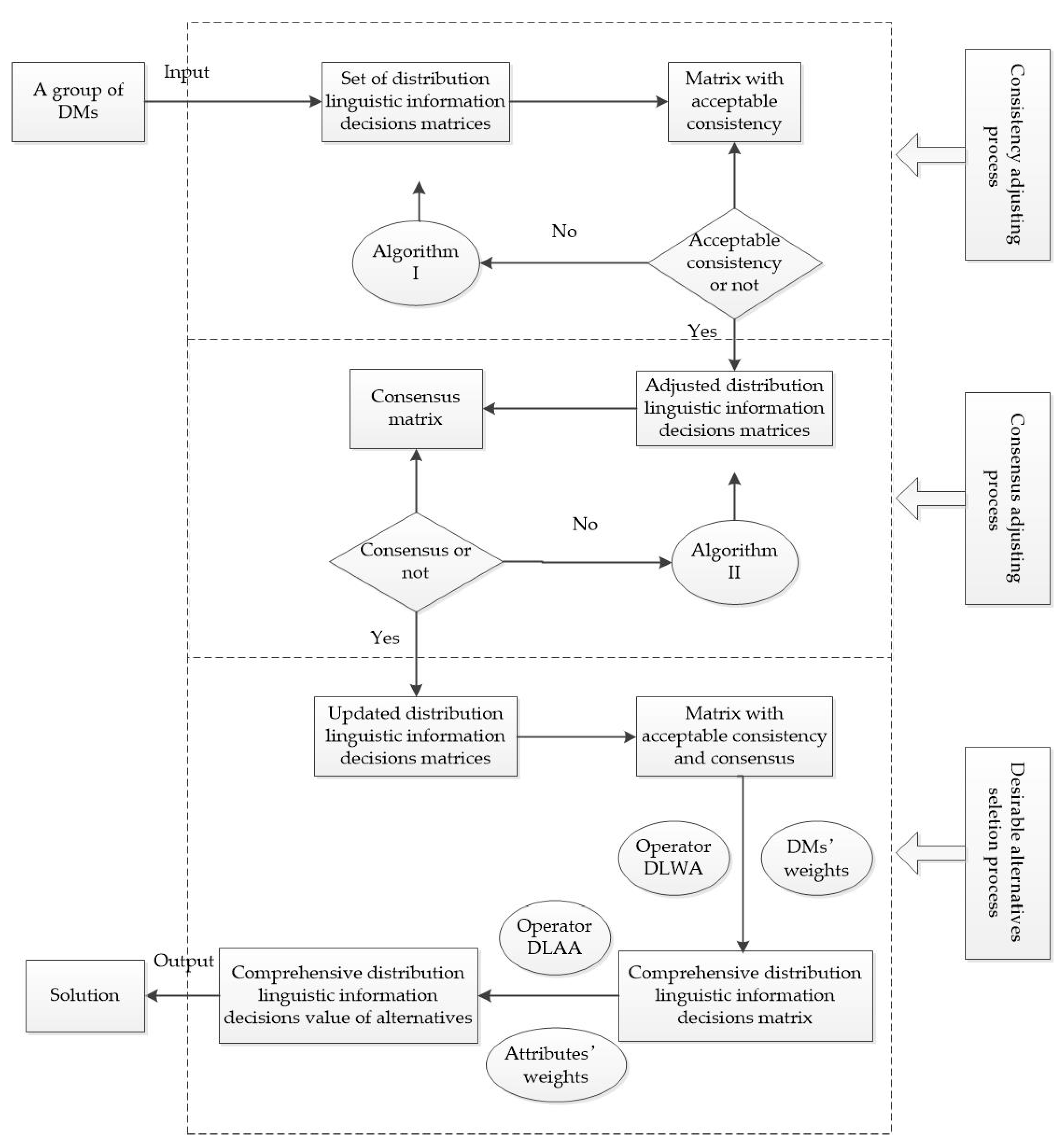
5. Distribution Linguistic Fuzzy GDM (DLFGDM) Method

DLFGDM method is a new decision support model developed by us, which can be divided into three stages as below:

Stage 1.

Improving internal consistency of experts: identify and adjust consistency level within experts, adjust original DLFPRs into new DLFPRs with acceptable consistency.

Stage 2.

Improving external consensus of experts: identify and adjust GCD of external experts, and output the consensus matrices.

Stage 3.

Making optimal selection: combine with known weights, DLFPR of acceptable consistency and consensus is aggregated by operators to form a comprehensive DLFPR and then integrate DLFEs into the final DLFE to sort.

The GDM problem involves the comparison and selection of alternatives. In the past research, [50] has proposed the probability linguistic weighted averaging (PLWA) operator to figure out the total aggregate.

We first aim to obtain the comprehensive DLFPR, thus we apply distribution linguistic weighted averaging (DLWA) operators which is based on PLWA operators [51,52].

If we know an important weight vector of experts, $\omega ={({\omega }_1,{\omega }_2,\dots ,{\omega }_n)}^T$, where ${\omega }_j\ge 0,{\displaystyle {\sum }_{j=1}^n{\omega }_j}=1$, then we use the DLWA operator to integrate DLFPRs ${\tilde{D}}_k={({\tilde{d}}_{ij}^k)}_{m\times n}(k=1,2,\dots ,l)$, where $d_{ij}^k=\left\{(s_{\xi },p_{ij(k)}^{(\xi )})|\xi =0,1,\dots ,2\tau ,0\le p_{ij(k)}^{(\xi )}\le 1,{\displaystyle \sum _{\xi =0}^{2\tau }{p}_{ij(k)}^{(\xi )}=1}\right\},$

$$\begin{array}{l}{d}_{ij}^{\prime } =DLWA({\tilde{d}}_{ij}^{(1)},{\tilde{d}}_{ij}^{(2)},\cdots ,{\tilde{d}}_{ij}^{(l)})\\ \hspace{1em} =w_1{\tilde{d}}_{ij}^{(1)}\oplus w_2{\tilde{d}}_{ij}^{(2)}\oplus \cdots \oplus w_n{\tilde{d}}_{ij}^{(l)}.\end{array}$$

(14)

Thus, we have a comprehensive DLFPR $D_{ij}^{\prime }={(d_{ij}^{\prime })}_{m\times n}$.

In the following, in order to obtain the best alternative from ranking order, an effective alternative sorting method is proposed by [50].

Suppose that an important weight vector, ${\omega }^{\prime }=({\omega }_1^{\prime },{\omega }_2^{\prime },\dots ,{\omega }_n^{\prime }{)}^T$, where ${\omega }_j^{\prime }=\frac{1}{n}$ is given, then we use the distribution linguistic arithmetic averaging (DLAA) operator to integrate the adjusted DLTSs of alternatives $a_i(i=1,2,\dots ,m)$

$$\begin{array}{l}{d}_i^{\prime } =DLAA(d_{i1}^{\prime },d_{i2}^{\prime },\dots ,d_{in}^{\prime })\\ \hspace{1em} =w_1{d}_{i1}^{\prime }\oplus w_2{d}_{i2}^{\prime }\oplus \cdots \oplus w_n{d}_{in}^{\prime }\\ \hspace{1em} =\frac{1}{n}(d_{i1}^{\prime }\oplus d_{i2}^{\prime }\oplus \cdots \oplus d_{in}^{\prime }).\end{array}$$

(15)

Therefore, we obtain the comprehensive DLFEs $\left\{d_1^{\prime },d_2^{\prime },\dots ,d_m^{\prime }\right\}$, then rank all alternatives $a_1,a_2,\dots ,a_m$ and make the most satisfactory choice.

The developed DLFGDM method is graphically shown in Figure 1.

6. Numerical Examples and Comparative Discussion

In this part, we apply the DLFGDM model to deal with the matter of equity incentive mode selection, then we provide a comparative analysis to present its advantages.

6.1. Application to Select the Best Equity Incentive Mode

With the continuous development of mixed ownership economy, the implementation of equity incentive in state-owned enterprises can combine the interests of managers and shareholders of the company, help to improve the internal governance of state-owned enterprises, enhance the competitiveness of state-owned enterprises, and add vitality to the long-run development of state-owned enterprises. Therefore, the choice of incentive mode is particularly important for realizing the goal of equity incentive. According to relevant documents [53], the stock incentive models can be divided into the following types: performance stock $(x_1)$, restricted stock $(x_2)$, virtual stock $(x_3)$. In addition, there are three evaluation attributes of stock incentive models: timeless $(c_1)$, binding force $(c_2)$, market risk $(c_3)$. Therefore, the state-owned enterprise invited three authoritative experts $\left\{e_1,e_2,e_3\right\}$ to compare and evaluate the four equity incentive modes and give their preferences. Let $S=\{s_0:very poor,s_1:poor,s_2:medium,s_3:good,$ $s_4:very good\}$ be a LDTS, where the threshold $\theta$ of group consensus index is 0.85. Besides, the cost of experts is $(g_1,g_2,g_3)=(1,3,4)$ [54,55]. At the same time, because of the complexity of thinking, the evaluation of experts is difficult to be expressed by numerical value, and FLPR is needed to describe it. For instance, DM $e_1$ compares restricted stock $(x_2)$ with virtual stock $(x_3)$ and gives an opinion that he/she is 20% sure that the linguistic preference level of restricted stock $(x_2)$ over virtual stock $(x_3)$ is very poor, 30% sure that restricted stock $(x_2)$ over virtual stock $(x_3)$ is poor, 40% sure that restricted stock $(x_2)$ over virtual stock $(x_3)$ is medium, 10% sure that restricted stock $(x_2)$ over virtual stock $(x_3)$ is good. Thus, the evaluation of experts on restricted stock $(x_2)$ over virtual stock $(x_3)$ can be expressed as a DLFE $h_{23}^1=\{(s_0,2),(s_1,0.3),(s_2,0.4)$$(s_3,0.1),(s_4,0)\}$. Therefore, through interviews with three experts and information acquisition based on the above methods, we obtain three distribution linguistic information decision-making matrices $H_k={(h_{ij}^k)}_{3\times 3}(k=1,2,3)$ as follows:

$$H_1=\left(\begin{array}{l}\begin{array}{ccc}\{(s_0,0),(s_1,0),(s_2,1),(s_3,0),(s_4,0)\}& \{(s_0,0.15),(s_1,0.15),(s_2,0.00),(s_3,0.60),(s_4,0.10)\}& \{(s_0,0.00),(s_1,0.20),(s_2,0.00),(s_3,0.45),(s_4,0.35)\}\end{array}\\ \begin{array}{ccc}\{(s_0,0.10),(s_1,0.60),(s_2,0.00),(s_3,0.15),(s_4,0.15)\}& \{(s_0,0),(s_1,0),(s_2,1),(s_3,0),(s_4,0)\}& \{(s_0,0.2),(s_1,0.3),(s_2,0.4),(s_3,0.1),(s_4,0.0)\}\end{array}\\ \begin{array}{ccc}\{(s_0,0.35),(s_1,0.45),(s_2,0.00),(s_3,0.20),(s_4,0.00)\}& \{(s_0,0.0),(s_1,0.1),(s_2,0.4),(s_3,0.3),(s_4,0.2)\}& \{(s_0,0),(s_1,0),(s_2,1),(s_3,0),(s_4,0)\}\end{array}\end{array}\right)$$

$$H_2=\left(\begin{array}{l}\begin{array}{ccc}\{(s_0,0),(s_1,0),(s_2,1),(s_3,0),(s_4,0)\}& \{(s_0,0.1),(s_1,0.1),(s_2,0.2),(s_3,0.3),(s_4,0.3)\}& \{(s_0,0.2),(s_1,0.5),(s_2,0.1),(s_3,0.1),(s_4,0.1)\}\end{array}\\ \begin{array}{ccc}\{(s_0,0.3),(s_1,0.3),(s_2,0.2),(s_3,0.1),(s_4,0.1)\}& \{(s_0,0),(s_1,0),(s_2,1),(s_3,0),(s_4,0)\}& \{(s_0,0.3),(s_1,0.2),(s_2,0.3),(s_3,0.2),(s_4,0.0)\}\end{array}\\ \begin{array}{ccc}\{(s_0,0.1),(s_1,0.1),(s_2,0.1),(s_3,0.5),(s_4,0.2)\}& \{(s_0,0.0),(s_1,0.2),(s_2,0.3),(s_3,0.2),(s_4,0.3)\}& \{(s_0,0),(s_1,0),(s_2,1),(s_3,0),(s_4,0)\}\end{array}\end{array}\right)$$

$$H_3=\left(\begin{array}{l}\begin{array}{ccc}\{(s_0,0),(s_1,0),(s_2,1),(s_3,0),(s_4,0)\}& \{(s_0,0.1),(s_1,0.1),(s_2,0.1),(s_3,0.6),(s_4,0.1)\}& \{(s_0,0.00),(s_1,0.35),(s_2,0.25),(s_3,0.20),(s_4,0.20)\}\end{array}\\ \begin{array}{ccc}\{(s_0,0.1),(s_1,0.6),(s_2,0.1),(s_3,0.1),(s_4,0.1)\}& \{(s_0,0),(s_1,0),(s_2,1),(s_3,0),(s_4,0)\}& \{(s_0,0.25),(s_1,0.00),(s_2,0.40),(s_3,0.35),(s_4,0.00)\}\end{array}\\ \begin{array}{ccc}\{(s_0,0.20),(s_1,0.20),(s_2,0.25),(s_3,0.35),(s_4,0.00)\}& \{(s_0,0.00),(s_1,0.35),(s_2,0.40),(s_3,0.00),(s_4,0.25)\}& \{(s_0,0),(s_1,0),(s_2,1),(s_3,0),(s_4,0)\}\end{array}\end{array}\right)$$

Part 1: Consistency improvement

Step 1. Based on Theorem 1 and Equation (2), we construct three DLFPRs ${\tilde{H}}_k={({\tilde{h}}_{ij}^k)}_{3\times 3}(k=1,2,3)$ with multiplicative consistency.

Step 2. Check the consistency index $CI$ of three DLFPRs $H_k={(h_{ij}^k)}_{3\times 3}(k=1,2,3)$ with $\overline{CI}=0.1$, $\delta =0.4$. According to Equation (10), we can have $CI(H_1)=0.1157$, $CI(H_2)=0.0741$, $CI(H_3)=0.1237$. Therefore, $CI(H_1)>\overline{CI}$, $CI(H_2)<\overline{CI}$, $CI(H_3)>\overline{CI}$.

Step 3. Generate the DLFPRs $H_1$ and $H_3$ on the basis of Algorithm 1. The updated DLFPRs ${\overline{H}}_1$ and ${\overline{H}}_3$ are shown below:

$${\overline{H}}_1=\left(\begin{array}{l}\begin{array}{ccc}\{(s_0,0),(s_1,0),(s_2,1),(s_3,0),(s_4,0)\}& \{(s_0,0.14),(s_1,0.13),(s_2,0.07),(s_3,0.48),(s_4,0.18)\}& \{(s_0,0.00),(s_1,0.20),(s_2,0.00),(s_3,0.45),(s_4,0.35)\}\end{array}\\ \begin{array}{ccc}\{(s_0,0.18),(s_1,0.48),(s_2,0.07),(s_3,0.13),(s_4,0.14)\}& \{(s_0,0),(s_1,0),(s_2,1),(s_3,0),(s_4,0)\}& \{(s_0,0.2),(s_1,0.3),(s_2,0.4),(s_3,0.1),(s_4,0.0)\}\end{array}\\ \begin{array}{ccc}\{(s_0,0.35),(s_1,0.45),(s_2,0.00),(s_3,0.20),(s_4,0.00)\}& \{(s_0,0.0),(s_1,0.1),(s_2,0.4),(s_3,0.3),(s_4,0.2)\}& \{(s_0,0),(s_1,0),(s_2,1),(s_3,0),(s_4,0)\}\end{array}\end{array}\right)$$

$$H_2=\left(\begin{array}{l}\begin{array}{ccc}\{(s_0,0),(s_1,0),(s_2,1),(s_3,0),(s_4,0)\}& \{(s_0,0.1),(s_1,0.1),(s_2,0.2),(s_3,0.3),(s_4,0.3)\}& \{(s_0,0.2),(s_1,0.5),(s_2,0.1),(s_3,0.1),(s_4,0.1)\}\end{array}\\ \begin{array}{ccc}\{(s_0,0.3),(s_1,0.3),(s_2,0.2),(s_3,0.1),(s_4,0.1)\}& \{(s_0,0),(s_1,0),(s_2,1),(s_3,0),(s_4,0)\}& \{(s_0,0.3),(s_1,0.2),(s_2,0.3),(s_3,0.2),(s_4,0.0)\}\end{array}\\ \begin{array}{ccc}\{(s_0,0.1),(s_1,0.1),(s_2,0.1),(s_3,0.5),(s_4,0.2)\}& \{(s_0,0.0),(s_1,0.2),(s_2,0.3),(s_3,0.2),(s_4,0.3)\}& \{(s_0,0),(s_1,0),(s_2,1),(s_3,0),(s_4,0)\}\end{array}\end{array}\right)$$

$${\overline{H}}_3=\left(\begin{array}{l}\begin{array}{ccc}\{(s_0,0),(s_1,0),(s_2,1),(s_3,0),(s_4,0)\}& \{(s_0,0.10),(s_1,0.13),(s_2,0.13),(s_3,0.46),(s_4,0.18)\}& \{(s_0,0.00),(s_1,0.35),(s_2,0.25),(s_3,0.20),(s_4,0.20)\}\end{array}\\ \begin{array}{ccc}\{(s_0,0.18),(s_1,0.46),(s_2,0.13),(s_3,0.13),(s_4,0.10)\}& \{(s_0,0),(s_1,0),(s_2,1),(s_3,0),(s_4,0)\}& \{(s_0,0.25),(s_1,0.08),(s_2,0.32),(s_3,0.30),(s_4,0.05)\}\end{array}\\ \begin{array}{ccc}\{(s_0,0.20),(s_1,0.20),(s_2,0.25),(s_3,0.35),(s_4,0.00)\}& \{(s_0,0.05),(s_1,0.30),(s_2,0.32),(s_3,0.08),(s_4,0.25)\}& \{(s_0,0),(s_1,0),(s_2,1),(s_3,0),(s_4,0)\}\end{array}\end{array}\right)$$

In addition, $CI({\overline{H}}_1)=0.0949<\overline{CI}$, $CI({\overline{H}}_3)=0.0850<\overline{CI}$.

Step 4. Let $H_1={\overline{H}}_1$, $H_3={\overline{H}}_3$, then $H_1,H_2,H_3$ are three DLFPRs with acceptable consistency.

Part 2: Consensus facilitation

Step 5. Construct the distance matrix $S{M}^{pq}={(s{m}_{ij}^{pq})}_{3\times 3},p,q=1,2,3$ in line accordance with the adjusted DLFPRs $H_1,H_2,H_3$ of acceptable consistency.

Step 6. Calculate GCD of three DLFPRs, then compare it with the group consensus index threshold $\theta =0.85$. Based on Equation (13), we have: $GCD=0.814<\theta$.

Step 7. Apply Algorithm 2 to ameliorate the consensus level. Among elements in $B={(b_{pq})}_{3\times 3}$, the smallest element is $b_{12}$.

Step 8. Chase down the smallest element $s{m}_{13}^{12}$ in $S{M}^{12}$, then we need to make adjustments to $d_{13}^1$ because the adjustment cost of $e_1$ is lower than $e_2$.

Step 9. Output the adjusted DLFPR $H_1^{\prime }$ as follows:

$$H_1^{\prime }=\left(\begin{array}{l}\begin{array}{ccc}\{(s_0,0),(s_1,0),(s_2,1),(s_3,0),(s_4,0)\}& \{(s_0,0.14),(s_1,0.13),(s_2,0.07),(s_3,0.48),(s_4,0.18)\}& \{(s_0,0.10),(s_1,0.40),(s_2,0.05),(s_3,0.25),(s_4,0.20)\}\end{array}\\ \begin{array}{ccc}\{(s_0,0.18),(s_1,0.48),(s_2,0.07),(s_3,0.13),(s_4,0.14)\}& \{(s_0,0),(s_1,0),(s_2,1),(s_3,0),(s_4,0)\}& \{(s_0,0.2),(s_1,0.3),(s_2,0.4),(s_3,0.1),(s_4,0.0)\}\end{array}\\ \begin{array}{ccc}\{(s_0,0.20),(s_1,0.25),(s_2,0.05),(s_3,0.40),(s_4,0.10)\}& \{(s_0,0.0),(s_1,0.1),(s_2,0.4),(s_3,0.3),(s_4,0.2)\}& \{(s_0,0),(s_1,0),(s_2,1),(s_3,0),(s_4,0)\}\end{array}\end{array}\right),$$

with $GC{D}^{\prime }=0.855>\theta$. Let $H_1=H_1^{\prime }$, then $H_1,H_2,H_3$ are three consensus matrices.

Part 3: Stock incentive models selection

Step 10. Utilize DLWA operator to integrate three DLFPRs into the comprehensive DLFPR $H^{\prime }$ with known expert weights $\omega ={(0.33,0.35,0.32)}^T$. $H^{\prime }$ is as shown below:

$$H^{\prime }=\left(\begin{array}{l}\begin{array}{ccc}\{(s_0,0),(s_1,0),(s_2,1),(s_3,0),(s_4,0)\}& \{(s_0,0.12),(s_1,0.12),(s_2,0.13),(s_3,0.41),(s_4,0.22)\}& \{(s_0,0.10),(s_1,0.42),(s_2,0.13),(s_3,0.18),(s_4,0.16)\}\end{array}\\ \begin{array}{ccc}\{(s_0,0.22),(s_1,0.41),(s_2,0.13),(s_3,0.12),(s_4,0.12)\}& \{(s_0,0),(s_1,0),(s_2,1),(s_3,0),(s_4,0)\}& \{(s_0,0.25),(s_1,0.20),(s_2,0.34),(s_3,20),(s_4,0.01)\}\end{array}\\ \begin{array}{ccc}\{(s_0,0.16),(s_1,0.18),(s_2,0.13),(s_3,0.42),(s_4,0.10)\}& \{(s_0,0.01),(s_1,0.20),(s_2,0.34),(s_3,0.20),(s_4,0.25)\}& \{(s_0,0),(s_1,0),(s_2,1),(s_3,0),(s_4,0)\}\end{array}\end{array}\right)$$

Step 11. Use DLAA operator to integrate the adjusted LDTSs of alternatives based on the adjusted DLFPR $H^{\prime }$. Then, we obtain the comprehensive DLFEs of stock incentive models as follows:

$$H^{*}=\left(\begin{array}{l}\{(s_0,0.07),(s_1,0.18),(s_2,0.42),(s_3,0.20),(s_4,0.13)\}\\ \{(s_0,0.16),(s_1,0.20),(s_2,0.49),(s_3,0.11),(s_4,0.04)\}\\ \{(s_0,0.06),(s_1,0.14),(s_2,0.48),(s_3,0.20),(s_4,0.11)\}\end{array}\right)$$

Step 12. Rank three stock incentive models $X=\{x_1,x_2,x_3\}$, we have $x_1\succ x_3\succ x_2$. Therefore, the best equity incentive mode is $x_1$.

6.2. Comparative Discussion

In this subsection, we compare our proposed DLFGDM method with other methods in [10,38].

6.2.1. Application of the Method in Zhang et al.

Zhang et al. [10] utilized the concept of distribution assessments in a LDTS and explored the consistency and consensus measures, then a consensus model is developed to help DMs ameliorate the consensus level among DLFPRs.

Step 1. Check that the group consensus level meets the requirements. Based on $\widetilde{CI}(H_p,H_q)=1-\tilde{d}(H_p,H_q)=1-\frac{1}{2n^2}{\displaystyle \sum _{j=1}^n{\displaystyle \sum _{i=1}^n{\displaystyle \sum _{\xi =0}^{2\tau }|p_{ij(p)}^{(\xi )}-p_{ij(q)}^{(\xi )}|}}}$, we can have $\widetilde{CI}(H_1,H_2)=0.867$, $\widetilde{CI}(H_1,H_3)=0.944, \widetilde{CI}(H_2,H_3)=0.928$. Let the threshold $\tilde{\theta }=0.9$, then $\widetilde{CI}(H_1,H_2)<\tilde{\theta }$, $\widetilde{CI}(H_1,H_3)>\tilde{\theta }, \widetilde{CI}(H_2,H_3)>\tilde{\theta }$, which means the DLFPRs of $e_1$ and $e_2$ need to be adjusted.

Step 2. Calculate identification rules $I{R}_{(1)},I{R}_{(2)}$ according to $I{R}_{(k)}=\frac{1}{z}{\displaystyle \sum _{q=1}^z\widetilde{CI}(H_{(k)},H_{(q)})}$, then we can obtain $I{R}_{(1)}=0.937, I{R}_{(2)}=0.932$ and $I{R}_{(1)}>I{R}_{(2)}$. Therefore, the DLFPR of $e_2$ need to be adjusted.

Step 3. Assume that the adjustment parameter $\beta$ of $e_2$ is $0.4$, then on the basis of $w=\frac{1-\beta }{z-1}$, we have: $w_2={(0.3,0.4,0.3)}^T$. Let ${\overline{\overline{H}}}_2={({\overline{\overline{h}}}_{ij,2})}_{3\times 3}$, where ${\overline{\overline{h}}}_{ij,2}=DAW{A}_{w_2}$$\{{\overline{\overline{h}}}_{ij,1},\dots ,{\overline{\overline{h}}}_{ij,4}\}$. After calculation, the ${\overline{\overline{H}}}_2$ is listed as below:

$${\overline{\overline{H}}}_2=\left(\begin{array}{l}\begin{array}{ccc}\{(s_0,0),(s_1,0),(s_2,1),(s_3,0),(s_4,0)\}& \{(s_0,0.12),(s_1,0.12),(s_2,0.09),(s_3,0.52),(s_4,0.15)\}& \{(s_0,0.05),(s_1,0.33),(s_2,0.12),(s_3,0.27),(s_4,0.23)\}\end{array}\\ \begin{array}{ccc}\{(s_0,0.15),(s_1,0.52),(s_2,0.09),(s_3,0.12),(s_4,0.12)\}& \{(s_0,0),(s_1,0),(s_2,1),(s_3,0),(s_4,0)\}& \{(s_0,0.24),(s_1,0.16),(s_2,0.38),(s_3,0.22),(s_4,0.00)\}\end{array}\\ \begin{array}{ccc}\{(s_0,0.23),(s_1,0.27),(s_2,0.12),(s_3,0.33),(s_4,0.05)\}& \{(s_0,0.00),(s_1,0.22),(s_2,0.38),(s_3,0.16),(s_4,0.24)\}& \{(s_0,0),(s_1,0),(s_2,1),(s_3,0),(s_4,0)\}\end{array}\end{array}\right)$$

In addition, ${\widetilde{CI}}^{\prime }(H_1,H_2)=0.933>\theta$, let $H_2={\overline{\overline{H}}}_2$ then three DLFPRs are consensus matrices.

Step 4. Use DLWA operator with known expert weight $\omega ={(0.33,0.35,0.32)}^T$, we can obtain a new comprehensive DLFPR $\overline{\overline{H}}$:

$$\overline{\overline{H}}=\left(\begin{array}{l}\begin{array}{ccc}\{(s_0,0),(s_1,0),(s_2,1),(s_3,0),(s_4,0)\}& \{(s_0,0.12),(s_1,0.12),(s_2,0.06),(s_3,0.57),(s_4,0.13)\}& \{(s_0,0.02),(s_1,0.29),(s_2,0.12),(s_3,0.31),(s_4,0.26)\}\end{array}\\ \begin{array}{ccc}\{(s_0,0.13),(s_1,0.57),(s_2,0.06),(s_3,0.12),(s_4,0.12)\}& \{(s_0,0),(s_1,0),(s_2,1),(s_3,0),(s_4,0)\}& \{(s_0,0.23),(s_1,0.16),(s_2,0.39),(s_3,0.22),(s_4,0.00)\}\end{array}\\ \begin{array}{ccc}\{(s_0,0.26),(s_1,0.31),(s_2,0.12),(s_3,0.29),(s_4,0.02)\}& \{(s_0,0.00),(s_1,0.22),(s_2,0.39),(s_3,0.16),(s_4,0.23)\}& \{(s_0,0),(s_1,0),(s_2,1),(s_3,0),(s_4,0)\}\end{array}\end{array}\right)$$

Step 5. Use DLAA operator with $\overline{\overline{H}}$ to integrate DLFEs, then we have:

$${\overline{\overline{H}}}^{*}=\left(\begin{array}{l}\{(s_0,0.05),(s_1,0.14),(s_2,0.40),(s_3,0.29),(s_4,0.12)\}\\ \{(s_0,0.12),(s_1,0.24),(s_2,0.49),(s_3,0.11),(s_4,0.04)\}\\ \{(s_0,0.09),(s_1,0.18),(s_2,0.49),(s_3,0.15),(s_4,0.09)\}\end{array}\right)$$

Therefore, we can conclude that $x_1\succ x_3\succ x_2$, and $x_1$ is the best equity incentive mode.

6.2.2. Application of the Method in Tang et al.

Tang et al. [38] used different types of numerical scale to connect DLPRs with FRL and multiplicative preference relation, and then gave the excepted consistency, and based on this, established the goal programming model to deduce the numerical scale of language terms.

Suppose that the scale functions of three DLFPRs $H_1,H_2,H_3$ are multiplicative. The optimization model can be established using the following methods:

For DLFPR $H_1$,

$$Min\hspace{0.17em}{M}^1={\pi }_{12}^{-}+{\pi }_{12}^{+}+{\pi }_{13}^{-}+{\pi }_{13}^{+}+{\pi }_{23}^{-}+{\pi }_{23}^{+}$$

$$\begin{array}{l}s.t.\\ \{\begin{array}{l}{\widehat{w}}_2\cdot (0.15q(l_0)+0.15q(l_1)+0.6q(l_2)+0.1q(l_3))-{\widehat{w}}_1+{\lambda }_{12}^{-}-{\lambda }_{12}^{+}=0\\ {\widehat{w}}_3\cdot (0.20q(l_0)+0.45q(l_3)+0.35q(l_4))-{\widehat{w}}_1+{\lambda }_{13}^{-}-{\lambda }_{13}^{+}=0\\ {\widehat{w}}_3\cdot (0.20q(l_0)+0.30q(l_1)+0.40q(l_2)+0.10q(l_3)-{\widehat{w}}_2+{\lambda }_{23}^{-}-{\lambda }_{23}^{+}=0\\ {\lambda }_{12}^{-},{\lambda }_{12}^{+},{\lambda }_{13}^{-},{\lambda }_{13}^{+},{\lambda }_{23}^{-},{\lambda }_{23}^{+}\ge 0\\ q(l_0)=1/3 and q(l_4)=3\\ q(l_{1-\alpha })\cdot q(l_{\alpha })=1,\alpha =0,1,2,3,4\\ \alpha \le q(l_{\alpha })\le (\alpha +2),\alpha =3,4\\ 1/(2-\alpha )\le q(l_{\alpha })\le 1/(-\alpha ),\alpha =0,1\\ 0<{\widehat{w}}_i\le 1,{\displaystyle {\sum }_{i=1}^3{\widehat{w}}_i}=1,i=1,2,3\end{array}\end{array}$$

By solving it, we can obtain that:

$$\begin{gathered} {\lambda }_{12}^{-}={\lambda }_{12}^{+}={\lambda }_{13}^{-}={\lambda }_{13}^{+}={\lambda }_{23}^{+}=0,{\lambda }_{23}^{-}=0.263,M^1=0.263;{\widehat{w}}^1={({\widehat{w}}_1,{\widehat{w}}_2,{\widehat{w}}_3)}^T={(0.388,0.420,0.192)}^T \\ \mathrm{and} q(l_0)=0.333,q(l_1)=0.5,q(l_2)=1,q(l_3)=2,q(l_4)=3 \end{gathered}$$

For DLFPR $H_2$,

$$M\mathrm{in}\hspace{0.17em}{M}^2={\pi }_{12}^{-}+{\pi }_{12}^{+}+{\pi }_{13}^{-}+{\pi }_{13}^{+}+{\pi }_{23}^{-}+{\pi }_{23}^{+}$$

$$\begin{array}{l}s.t.\\ \{\begin{array}{l}{\widehat{w}}_2\cdot (0.1q(l_0)+0.1q(l_1)+0.2q(l_2)+0.3q(l_3)+0.3q(l_4))-{\widehat{w}}_1+{\lambda }_{12}^{-}-{\lambda }_{12}^{+}=0\\ {\widehat{w}}_3\cdot (0.2q(l_0)+0.5q(l_1)+0.1q(l_2)+0.1q(l_3)+0.1q(l_4))-{\widehat{w}}_1+{\lambda }_{13}^{-}-{\lambda }_{13}^{+}=0\\ {\widehat{w}}_3\cdot (0.3q(l_0)+0.2q(l_1)+0.3q(l_2)+0.2q(l_3)-{\widehat{w}}_2+{\lambda }_{23}^{-}-{\lambda }_{23}^{+}=0\\ {\lambda }_{12}^{-},{\lambda }_{12}^{+},{\lambda }_{13}^{-},{\lambda }_{13}^{+},{\lambda }_{23}^{-},{\lambda }_{23}^{+}\ge 0\\ q(l_0)=1/3 and q(l_4)=3\\ q(l_{1-\alpha })\cdot q(l_{\alpha })=1,\alpha =0,1,2,3,4\\ \alpha \le q(l_{\alpha })\le (\alpha +2),\alpha =3,4\\ 1/(2-\alpha )\le q(l_{\alpha })\le 1/(-\alpha ),\alpha =0,1\\ 0<{\widehat{w}}_i\le 1,{\displaystyle {\sum }_{i=1}^3{\widehat{w}}_i}=1,i=1,2,3\end{array}\end{array}$$

By solving it, we can obtain that:

$$\begin{gathered} {\lambda }_{12}^{+}={\lambda }_{12}^{-}={\lambda }_{13}^{-}={\lambda }_{13}^{+}={\lambda }_{23}^{-}=0,{\lambda }_{23}^{+}=0.158,M^2=0.158;{\widehat{w}}^2={({\widehat{w}}_1,{\widehat{w}}_2,{\widehat{w}}_3)}^T={(0.377,0.212,0.411)}^T \\ \mathrm{and} q(l_0)=0.333,q(l_1)=0.5,q(l_2)=1,q(l_3)=2,q(l_4)=3. \end{gathered}$$

For DLFPR $H_3$,

$$Min\hspace{0.17em}{M}^2={\pi }_{12}^{-}+{\pi }_{12}^{+}+{\pi }_{13}^{-}+{\pi }_{13}^{+}+{\pi }_{23}^{-}+{\pi }_{23}^{+}$$

$$\begin{array}{l}s.t.\\ \{\begin{array}{l}{\widehat{w}}_2\cdot (0.10q(l_0)+0.10q(l_1)+0.10q(l_2)+0.60q(l_3)+0.10q(l_4))-{\widehat{w}}_1+{\lambda }_{12}^{-}-{\lambda }_{12}^{+}=0\\ {\widehat{w}}_3\cdot (0.35q(l_1)+0.25q(l_2)+0.20q(l_3)+0.20q(l_4))-{\widehat{w}}_1+{\lambda }_{13}^{-}-{\lambda }_{13}^{+}=0\\ {\widehat{w}}_3\cdot (0.25q(l_0)+0.40q(l_2)+0.35q(l_3)-{\widehat{w}}_2+{\lambda }_{23}^{-}-{\lambda }_{23}^{+}=0\\ {\lambda }_{12}^{-},{\lambda }_{12}^{+},{\lambda }_{13}^{-},{\lambda }_{13}^{+},{\lambda }_{23}^{-},{\lambda }_{23}^{+}\ge 0\\ q(l_0)=1/3 and q(l_4)=3\\ q(l_{1-\alpha })\cdot q(l_{\alpha })=1,\alpha =0,1,2,3,4\\ \alpha \le q(l_{\alpha })\le (\alpha +2),\alpha =3,4\\ 1/(2-\alpha )\le q(l_{\alpha })\le 1/(-\alpha ),\alpha =0,1\\ 0<{\widehat{w}}_i\le 1,{\displaystyle {\sum }_{i=1}^3{\widehat{w}}_i}=1,i=1,2,3\end{array}\end{array}$$

By solving it with similar methods, we can learn that:

$$\begin{gathered} {\lambda }_{12}^{+}={\lambda }_{12}^{-}={\lambda }_{13}^{+}={\lambda }_{23}^{-}={\lambda }_{23}^{+}=0,{\lambda }_{13}^{-}=0.060,M^3=0.060;{\widehat{w}}^3={({\widehat{w}}_1,{\widehat{w}}_2,{\widehat{w}}_3)}^T={(0.518,0.308,0.174)}^T, \\ \mathrm{and} q(l_0)=0.333,q(l_1)=0.5,q(l_2)=1,q(l_3)=2,q(l_4)=3. \end{gathered}$$

Using the direct evaluation method to determine the expert weights $\omega ={(0.33,0.35,0.32)}^T$, the following ranking matrix is obtained.

$$\begin{array}{l}\hspace{1em}\hspace{1em}\hspace{1em}\hspace{1em}{\widehat{w}}^1\hspace{1em} {\widehat{w}}^2\hspace{1em} {\widehat{w}}^3\hspace{1em}\hspace{1em}\hspace{1em} \omega \hspace{1em}\hspace{1em}\hspace{1em}\hspace{1em}{\widehat{w}}^{\prime }\\ \begin{array}{c}{x}_1\\ x_2\\ x_3\end{array}\begin{array}{c}\to \\ \to \\ \to \end{array}\left[\begin{array}{l}\begin{array}{ccc}0.388& 0.377& 0.518\end{array}\\ \begin{array}{ccc}0.420& 0.212& 0.308\end{array}\\ \begin{array}{ccc}0.192& 0.411& 0.174\end{array}\end{array}\right]\times \left[\begin{array}{l}0.33\\ 0.35\\ 0.32\end{array}\right]=\left[\begin{array}{l}0.423\\ 0.329\\ 0.248\end{array}\right]\end{array}$$

Therefore, we can obtain the final ranking $x_1\succ x_2\succ x_3$, and consider $x_1$ as the best equity incentive mode.

On the basis of the above results, we can obtain that the three methods make the same decision and all choose $x_1$ as the best equity incentive mode. Therefore, the method developed in this paper is effective and has certain practical significance. In the following, we summarize the advantages of this method through comparative discussion:

• It is essential to improve the level of consistency and consensus in GDM. However, Zhang et al. [10] did not check the consistency of the original DLFPRs, but directly carried out the consensus degree test by defining $\widetilde{CI}$, ignoring the consistency adjustment within the experts, and then directly used the weighted average method to update and adjust, which results in insufficient retention of the original language information of the experts and a large range of changes. Therefore, the developed DLFGDM method includes not only the consistency identification but also the consistency improvement method, so the application of it will be more reliable.
• Compared to the method of Tang et al. [38], our scheme has a different ranking. However, Tang et al. [38] only use the goal programming model based on expected consistency for adjustment, without consensus test and consensus improvement. Due to the influence of subjective and objective factors, the evaluation information proposed by experts may differ greatly, and there may be differences between them. Therefore, the direct application of the established expert weight to the final evaluation ranking may lead to the results being not reliable and lack of rationality. Our DLFGDM method measures and adjusts the consensus degree, and uses the weighted average operator to form a comprehensive consensus matrix to comprehensively deal with the experts’ opinions, which is more reasonable, more reliable and has a wider application prospect.

In addition, due to the focus of the paper and the convenience of calculation, this paper only selects the situation where three experts make decisions. When the number of DMs increases, more DLFPRs will be provided. We will conduct the identification adjustment of consistency level and consensus degree, so that the internal and external consensus of experts can be reached, and the final scheme ordering will be formed to make the optimal decision. When decisions are made in large groups, consistency and consensus are greatly improved, and the results are more reasonable and reliable. In the future, we will also take large-scale group decision making as one of the research directions.

7. Conclusions

Nowadays, consistency and consensus decision-making are very important to eliminate internal and external differences among experts and form reliable decision results. In this study, we introduce the concept of DLFPRs, consider the distance between expert evaluation and constructed consistency evaluation, and propose a new consistency recognition and adjustment algorithm. After ensuring the acceptable consistency, the consensus degree can be improved to reach a higher acceptable consensus level. Then DLWA operator is used to obtain the comprehensive evaluation matrix. Finally, DLAA operator is used to obtain fuzzy distributed language elements and order them.

The results of this study are divided into the following aspects:

• Based on the new distance formula, a new consistency index is introduced.
• The definition of multiplicative consistency of DLFPR is presented to include only the variation of distributed language evaluation probability. A new consistency adjustment algorithm is proposed, which preserves the original appraisement information as far as possible and adjusts the lowest consistency element each time.
• A new consensus degree and a consensus promotion algorithm are developed by considering the costs of experts.
• Two operators are used to integrate the distribution linguistic elements to derive alternative sorting.

In general, the DLFGDM method developed by us can transform and analyze the evaluation information provided by experts. In case of internal and external differences between experts, we utilize the identifying and adjusting algorithm to improve the internal consistency and external consensus, including the cost of experts considered. This is so that we can solve GDM problems better and make the most reasonable and reliable decision.

At the same time, this study also has some deficiencies:

• Without considering the limited knowledge and complex problems in real decision making, the evaluation information may be incomplete.
• The predetermined expert weights and attribute weights remain unchanged, which lacks certain rationality.

Therefore, in the future, we should further study the multi-granularity terms of different experts [56], multi-standard decision-making methods [57], large-scale group decision-making [58,59], and consider the psychological characteristics of regret aversion of experts [49], so that we can expand the application scope of decision support model and apply it to more complex and diverse situations.

References

- Zhang, L.L.; Yuan, J.J.; Gao, X.Y.; Jiang, D.W. Public transportation development decision-making under public participation: A large-scale group decision-making method based on fuzzy preference relations. Technol. Forecast Soc. Chang. 2021, 172, 121020. [Google Scholar] [CrossRef]
- Chen, Z.S.; Liu, X.L.; Chin, K.S.; Pedrycz, W.; Tsui, K.L.; Skibniewski, M.J. Online-review analysis based large-scale group decision-making for determining passenger demands and evaluating passenger satisfaction: Case study of high-speed rail system in China. Inf. Fusion. 2021, 69, 22–39. [Google Scholar] [CrossRef]
- Wang, L.J.; Chen, J. Research on Equity incentive decision-making based on Rough set Theory. China Circ. Econ. 2017, 23, 51–52. [Google Scholar]
- Lovsky, S.A. Decision-making with a fuzzy preference relation. Fuzzy Sets Syst. 1978, 1, 155–167. [Google Scholar]
- Liu, C.-H.; Liu, B. Using DANP-mV model to improve the paid training measures for travel agents amid the COVID-19 pandemic. Mathematics 2021, 9, 1924. [Google Scholar] [CrossRef]
- Yager, R.R.; Abbasov, A.M. Pythagorean membership grades, complex numbers, and decision making. Int. J. Intell. Syst. 2013, 28, 436–452. [Google Scholar] [CrossRef]
- Wu, P.; Zhou, L.G.; Zheng, T.; Chen, H.Y. A Fuzzy Group Decision Making and Its Application Based on Compatibility with Multiplicative Trapezoidal Fuzzy Preference Relations. Int. J. Fuzzy Syst. 2017, 19, 683–701. [Google Scholar] [CrossRef]
- Zadeh, L.A. The concept of a linguistic variable and its application to approximate reasoning-I. Inf. Sci. 1975, 8, 199–249. [Google Scholar] [CrossRef]
- Herrera, F.; Martinez, L. A 2-tuple fuzzy linguistic representation model for computing with words. IEEE Trans. Fuzzy Syst. 2000, 8, 746–752. [Google Scholar]
- Zhang, G.Q.; Dong, Y.C.; Xu, Y.F. Consistency and consensus measures for linguistic preference relations based on distribution assessments. Inf. Fus. 2014, 17, 46–55. [Google Scholar] [CrossRef]
- Guo, W.T.; Huynh, V.N.; Sriboonchitta, S. A proportional linguistic distribution based model for multiple attribute decision making under linguistic uncertainty. Ann. Oper. Res. 2017, 256, 305–328. [Google Scholar] [CrossRef]
- Huang, J.; Li, Z.J.; Liu, H.C. New approach for failure mode and effect analysis using linguistic distribution assessments and TODIM method. Reliab. Eng. Syst. Saf. 2017, 167, 302–309. [Google Scholar] [CrossRef]
- Wu, Y.Z.; Li, C.C.; Chen, X.; Dong, Y.C. Group decision making based on linguistic distributions and hesitant assessments: Maximizing the support degree with an accuracy constraint. Inf. Fusion. 2018, 41, 151–160. [Google Scholar] [CrossRef]
- Liang, Y.Y.; Ju, Y.B.; Qin, J.D.; Pedrycz, W. Multi-granular linguistic distribution evidential reasoning method for renewable energy project risk assessment. Inf. Fusion. 2021, 65, 147–164. [Google Scholar] [CrossRef]
- Ju, Y.B.; Liang, Y.Y.; Luis, M.; Gonzalez, E.D.R.S.; Giannakis, M.; Dong, P.W.; Wang, A.H. A new framework for health-care waste disposal alternative selection under multi-granular linguistic distribution assessment environment. Comput. Ind. Eng. 2020, 145, 106489. [Google Scholar] [CrossRef]
- Wang, X.K.; Wang, Y.T.; Zhang, H.Y.; Wang, J.Q.; Li, L.; Goh, M. An asymmetric trapezoidal cloud-based linguistic group decision-making method under unbalanced linguistic distribution assessments. Comput. Ind. Eng. 2021, 160, 107457. [Google Scholar] [CrossRef]
- Dong, Y.; Hong, W.; Xu, Y. Measuring consistency of linguistic preference relations: A 2-tuplelinguistic approach. Soft Comput. 2013, 17, 2117–2130. [Google Scholar] [CrossRef]
- Dong, Y.; Xu, Y.; Li, H. On consistency measures of linguistic preference relations. Eur. J. Oper. Res. 2008, 189, 430–444. [Google Scholar] [CrossRef]
- Jin, F.; Ni, Z.; Chen, H.; Li, Y. Approaches to decision making with linguistic preference relations based on additive consistency. Appl. Soft Comput. 2016, 49, 71–80. [Google Scholar] [CrossRef]
- Jin, F.; Ni, Z.; Pei, L.; Chen, H.; Tao, Z.; Zhu, X.; Ni, L. Approaches to group decision making with linguistic preference relations based on multiplicative consistency. Comput. Ind. Eng. 2017, 114, 69–79. [Google Scholar] [CrossRef]
- Tang, X.A.; Peng, Z.L.; Zhang, Q.; Pedrycz, W.; Yang, S.L. Consistency and consensus-driven models to personalize individual semantics of linguistic terms for supporting group decision making with distribution linguistic preference relations. Knowl. Based. Syst. 2019, 189, 105087. [Google Scholar] [CrossRef]
- Zhao, M.; Ma, X.Y.; Wei, D.W. A method considering and adjusting individual consistency and group consensus for group decision making with incomplete linguistic preference relations. Appl. Soft Comput. 2017, 54, 322–346. [Google Scholar] [CrossRef]
- Wang, H.; Xu, Z.S. Interactive algorithms for improving incomplete linguistic preference relations based on consistency measures. Appl. Soft Comput. 2016, 42, 66–79. [Google Scholar] [CrossRef]
- Cai, M.; Gong, Z.W.; Cao, J. The consistency measures of multi-granularity linguistic group decision making. J. Intell. Fuzzy Syst. 2015, 29, 609–618. [Google Scholar]
- Zhao, S.H.; Dong, Y.C.; Wu, S.Q.; Luis, M. Linguistic scale consistency issues in multi-granularity decision making contexts. Appl. Soft Comput. 2021, 101, 107035. [Google Scholar] [CrossRef]
- Wang, Y.C.; Tsai, H.R.; Chen, T. A selectively fuzzified back propagation network approach for precisely estimating the cycle time range in wafer fabrication. Mathematics 2021, 9, 1430. [Google Scholar] [CrossRef]
- Gong, K.X.; Chen, C.F.; Wei, Y. The consistency improvement of probabilistic linguistic hesitant fuzzy preference relations and their application in venture capital group decision making. J. Intell. Fuzzy Syst. 2019, 37, 2925–2936. [Google Scholar] [CrossRef]
- Gao, J.; Xu, Z.S.; Liang, Z.L.; Liao, H.C. Expected consistency-based emergency decision making with incomplete probabilistic linguistic preference relations. Knowl. Based. Syst. 2019, 176, 15–28. [Google Scholar] [CrossRef]
- Yodmun, S.; Witayakiattilerd, W.; Averbakh, I.L. Stock selection into portfolio by fuzzy quantitative analysis and fuzzy multicriteria decision making. Adv. Oper. Res. 2016. [Google Scholar] [CrossRef] [Green Version]
- Zhang, B.W.; Liang, H.M.; Gao, Y.; Zhang, G.Q. The optimization-based aggregation and consensus with minimum-cost in group decision making under incomplete linguistic distribution context. Knowl. Based. Syst. 2018, 162, 92–102. [Google Scholar] [CrossRef]
- Liu, N.N.; He, Y.; Xu, Z.S. A new approach to deal with consistency and consensus issues for hesitant fuzzy linguistic preference relations. Appl. Soft Comput. 2019, 76, 400–415. [Google Scholar] [CrossRef]
- Yao, S.B. A New Distance-based consensus reaching model for multi-attribute group decision-making with linguistic distribution assessments. Int. J. Comput. Int. Syst. 2018, 12, 395–409. [Google Scholar] [CrossRef] [Green Version]
- Chen, Z.S.; Zhang, X.; Pedrycz, W.; Wang, X.J.; Martinez, L. K-means clustering for the aggregation of HFLTS possibility distributions: N-two-stage algorithmic paradigm. Knowl. Based. Syst. 2021, 227, 107230. [Google Scholar] [CrossRef]
- Gao, Y.; Li, D.S. A consensus model for heterogeneous multi-attribute group decision making with several attribute sets. Expert Syst. Appl. 2019, 125, 69–80. [Google Scholar] [CrossRef]
- Jin, F.F.; Garg, H.; Pei, L.D.; Liu, J.P.; Chen, H.Y. Multiplicative consistency adjustment model and data envelopment analysis-driven decision-making process with probabilistic hesitant fuzzy preference relations. Int. J. Fuzzy Syst. 2020, 22, 2319–2332. [Google Scholar] [CrossRef]
- Yu, W.Y.; Zhang, Z.; Zhong, Q.Y. Consensus reaching for MAGDM with multi-granular hesitant fuzzy linguistic term sets: A minimum adjustment-based approach. Ann. Oper. Res. 2021, 300, 443–466. [Google Scholar] [CrossRef]
- Wu, T.; Liu, X.W.; Qin, J.D.; Herrera, F. Consensus evolution networks: A consensus reaching tool for managing consensus thresholds in group decision making. Inf. Fusion. 2019, 52, 375–388. [Google Scholar] [CrossRef]
- Tang, X.A.; Zhang, Q.; Peng, Z.L.; Yang, S.L.; Pedrycz, W. Derivation of personalized numerical scales from distribution linguistic preference relations: An expected consistency-based goal programming approach. Neural. Comput. Appl. 2019, 31, 8769–8786. [Google Scholar] [CrossRef]
- Li, C.C.; Dong, Y.C.; Herrera, F.; Herrera-Viedma, E.; Martínez, L. Personalized individual semantics in computing with words for supporting linguistic group decision making: An application on consensus reaching. Inf. Fusion. 2017, 33, 29–40. [Google Scholar] [CrossRef] [Green Version]
- Martínez, L.; Herrera, F. Challenges of computing with words in decision making. Inf. Sci. 2014, 258, 218–219. [Google Scholar] [CrossRef]
- Martínez, L.; Ruan, D.; Herrera, F. Computing with words in decision support systems: An overview on models and applications. Int. J. Comput. Int. Syst. 2010, 3, 382–395. [Google Scholar]
- Liu, J.; Martínez, L.; Wang, H.M.; Rodríguez, R.M.; Novozhilov, V. Computing with words in risk assessment. Int. J. Comput. Int. 2010, 3, 396–419. [Google Scholar]
- Rodríguez, R.M.; Martínez, L.; Herrera, F. Hesitant fuzzy linguistic term sets for decision making. IEEE Trans. Fuzzy Syst. 2012, 20, 109–119. [Google Scholar] [CrossRef]
- Labella, Á.; Liu, H.B.; Rodríguez, R.M.; Martínez, L. A cost consensus metric for consensus reaching processes based on a comprehensive minimum cost model. Eur. J. Oper. Res. 2020, 281, 316–331. [Google Scholar] [CrossRef]
- Romero, Á.L.; Rodríguez, R.M.; Martínez, L. Computing with comparative linguistic expressions and symbolic translation for decision making: ELICIT information. IEEE Trans. Fuzzy Syst. 2020, 28, 2510–2522. [Google Scholar] [CrossRef]
- Zhang, Z.M.; Chen, S.M. Group decision making based on acceptable multiplicative consistency and consensus of hesitant fuzzy linguistic preference relations. Inf. Sci. 2020, 541, 531–550. [Google Scholar] [CrossRef]
- Dong, Y.C.; Xu, Y.F. Consistency measures of linguistic preference relations and its properties in group decision making. Int. Conf. Fuzzy Syst. Knowl. Discov. 2006, 4223, 501–511. [Google Scholar]
- Jin, F.F.; Cao, M.; Liu, J.P.; Luis, M.; Chen, H.Y. Consistency and trust relationship-driven social network group decision-making method with probabilistic linguistic information. Appl. Soft Comput. 2021, 103, 107170. [Google Scholar] [CrossRef]
- Jin, F.F.; Liu, J.P.; Zhou, L.G.; Luis, M. Consensus-based linguistic distribution large-scale group decision making using statistical inference and regret theory. Group Decis. Negot. 2021, 30, 813–845. [Google Scholar] [CrossRef] [PubMed]
- Bai, C.Z.; Zhang, R.; Qian, L.X.; Wu, Y.N. Comparisons of probabilistic linguistic term sets for multi-criteria decision making. Knowl. Based. Syst. 2017, 119, 284–291. [Google Scholar] [CrossRef]
- Pang, Q.; Wang, H.; Xu, Z. Probabilistic linguistic term sets in multi-attribute group decision making. Inf. Sci. 2016, 369, 128–143. [Google Scholar] [CrossRef]
- Gou, X.; Xu, Z. Novel basic operational laws for linguistic terms, hesitant fuzzy linguistic term sets and probabilistic linguistic term sets. Inf. Sci. 2016, 372, 407–427. [Google Scholar] [CrossRef]
- Dong, H.J. On the selection of equity incentive mode in mixed reform of state-owned enterprises. Financ. Superv. 2019, 7, 97–102. [Google Scholar]
- Ben-Arieh, D.; Easton, T.; Evans, B. Minimum cost consensus with quadratic cost functions. IEEE Trans. Syst. Man Cybern. 2009, 39, 210–217. [Google Scholar] [CrossRef]
- Gong, Z.W.; Xu, X.X.; Guo, W.W.; Herrera-Viedma, E.; Cabrerizo, F.J. Minimum cost consensus modelling under various linear uncertain-constrained scenarios. Inf. Fusion. 2021, 66, 1–17. [Google Scholar] [CrossRef]
- Morente-Molinera, J.A.; Pérez, I.J.; Urena, M.R.; Herrera-Viedma, E. On multi-granular fuzzy linguistic modeling in group decision making problems: A systematic review. Knowl. Based. Syst. 2015, 74, 49–60. [Google Scholar] [CrossRef]
- Peng, H.G.; Wang, J.Q.; Zhang, H.Y. Multi-criteria outranking method based on probability distribution with probabilistic linguistic information. Comput. Ind. Eng. 2020, 141, 106318. [Google Scholar] [CrossRef]
- Li, S.L.; Wei, C.P. A large-scale group decision making approach in healthcare service based on sub-group weighting model and hesitant fuzzy linguistic information. Comput. Ind. Eng. 2020, 144, 106444. [Google Scholar] [CrossRef]
- Ren, R.X.; Tang, M.; Liao, H.C. Managing minority opinions in micro-grid planning by a social network analysis-based large scale group decision making method with hesitant fuzzy linguistic information. Knowl Based Syst. 2019, 189, 105060. [Google Scholar] [CrossRef]
Figure 1.
The developed DLFGDM method.
Publisher’s Note: MDPI stays neutral with regard to jurisdictional claims in published maps and institutional affiliations. |
© 2021 by the authors. Licensee MDPI, Basel, Switzerland. This article is an open access article distributed under the terms and conditions of the Creative Commons Attribution (CC BY) license (https://creativecommons.org/licenses/by/4.0/).
Share and Cite
MDPI and ACS Style
Jin, F.; Li, C.; Liu, J.; Zhou, L. Distribution Linguistic Fuzzy Group Decision Making Based on Consistency and Consensus Analysis. Mathematics 2021, 9, 2457. https://doi.org/10.3390/math9192457
AMA Style
Jin F, Li C, Liu J, Zhou L. Distribution Linguistic Fuzzy Group Decision Making Based on Consistency and Consensus Analysis. Mathematics. 2021; 9(19):2457. https://doi.org/10.3390/math9192457
Chicago/Turabian StyleJin, Feifei, Chang Li, Jinpei Liu, and Ligang Zhou. 2021. "Distribution Linguistic Fuzzy Group Decision Making Based on Consistency and Consensus Analysis" Mathematics 9, no. 19: 2457. https://doi.org/10.3390/math9192457
Note that from the first issue of 2016, this journal uses article numbers instead of page numbers. See further details here.