Grid Frequency and Amplitude Control Using DFIG Wind Turbines in a Smart Grid


1
Engineering School of Gipuzkoa, University of the Basque Country, Otaola Hirib. 29, 20600 Eibar, Spain
2
Engineering School of Vitoria, University of the Basque Country, Nieves Cano 12, 01006 Vitoria, Spain
3
Engineering School of Gipuzkoa, University of the Basque Country, Europa Plaza 1, 20018 Donostia, Spain
*
Author to whom correspondence should be addressed.
Mathematics 2021, 9(2), 143; https://doi.org/10.3390/math9020143
Submission received: 29 November 2020
/
Revised: 5 January 2021
/
Accepted: 8 January 2021
/
Published: 11 January 2021
(This article belongs to the Special Issue Advanced Modeling and Research in Hybrid Microgrid Control and Optimization)
Abstract
:Wind-generated energy is a fast-growing source of renewable energy use across the world. A dual-feed induction machine (DFIM) employed in wind generators provides active and reactive, dynamic and static energy support. In this document, the droop control system will be applied to adjust the amplitude and frequency of the grid following the guidelines established for the utility’s smart network supervisor. The wind generator will work with a maximum deloaded power curve, and depending on the reserved active power to compensate the frequency drift, the limit of the reactive power or the variation of the voltage amplitude will be explained. The aim of this paper is to show that the system presented theoretically works correctly on a real platform. The real-time experiments are presented on a test bench based on a 7.5 kW DFIG from Leroy Somer’s commercial machine that is typically used in industrial applications. A synchronous machine that emulates the wind profiles moves the shaft of the DFIG. The amplitude of the microgrid voltage at load variations is improved by regulating the reactive power of the DFIG and this is experimentally proven. The contribution of the active power with the characteristic of the droop control to the load variation is made by means of simulations. Previously, the simulations have been tested with the real system to ensure that the simulations performed faithfully reflect the real system. This is done using a platform based on a real-time interface with the DS1103 from dSPACE.
1. Introduction
Wind energy is progressively gaining importance in the world’s electricity production, with important engineering aspects to be addressed for its integration into conventional electricity grids. In fact, it contributes about 7% of total energy production worldwide and onshore and offshore wind energy together would generate more than a third of all electricity needs, becoming the main source of generation by 2050 [1].
Recently, some studies have been developed in order to analyze the installation of small wind turbines in urban areas. Installing wind turbines in all the possible extents can mitigate the rising energy demand. Built-up areas possess high potential for wind energy, including the rooftop of high-rise buildings, railway track, the region between or around multistoried buildings, and city roads. However, harnessing wind energy from these areas is quite challenging due to dynamic environments and turbulence for higher roughness on urban surfaces [2]. Some studies have been done in order to estimate the wind resource in an urban area [3,4]. These studies evaluate the urban wind resource by employing a physically-based empirical model to link wind observations at a conventional meteorological site to those acquired at urban sites. The approach is based on urban climate research that has examined the effects of varying surface roughness on the wind-field between and above buildings. These papers aim to provide guidance for optimizing the placement of small wind turbines in urban areas by developing an improved method of estimating the wind resource across a wide urban area.
There are different types of wind turbines like induction generator [5] or permanent magnet synchronous generators [6,7] based wind turbines, however the synchronous generators are usually used for a small-scale wind turbines.
In addition, the DFIM is the most commonly installed type of generator in wind turbines to date.
DFIG generators provide access to the rotor windings and regulating the rotor voltage, the generator active and reactive powers are fully controllable. Therefore, the design and implementation of a new control scheme for a DFIG based wind turbine system has attracted the attention of several authors in the last years [8,9,10,11,12].
The main reason for using the doubly fed induction generator is that the power converters have to manage only a fraction of the total system power, about 30%.
For this reason, there are fewer losses in the power electronics unit than in a full-power converter topology. The reduction in costs due to the use of a smaller inverter is another significant factor [13].
The regulation of the active and reactive powers in decoupled form with the DFIG is regulated using the field-oriented control (FOC) technique [14,15,16,17,18,19].
A smart grid has among its goals one dedicated to providing a more robust, efficient, and flexible electric power system [20,21]. In the last decade, the model predictive control (MPC) has been applied to microgrid systems to optimally schedule and control the microgrid, owing to the advantages of MPC such as fast response and robustness against parameter uncertainties. In the work presented in [22], a stochastic model predictive control framework to optimally schedule and control the microgrid with large scale renewable energy sources is proposed. This microgrid consists of fuel cell-based, wind turbines, PV generators, battery/thermal energy storage system gas fired boilers, and various types of electrical and thermal loads scheduled according to the demand response policy. In the work presented in [23], the authors propose a MPC for regulating frequency in stand-alone microgrids. This work analyzes the impact of system parameters on the control performance of MPC for frequency regulation, using a typical stand-alone microgrid, which consists of a diesel engine generator, an energy storage system, a wind turbine generator, and a load. A novel sensorless model predictive control (MPC) strategy of a wind-driven doubly fed induction generator (DFIG) connected to a dc microgrid is proposed in [24]. In this work, the MPC strategy has been used as a current controller to overcome the weaknesses of the inner control loop and to consider the discrete-time operation of the voltage source converter that feeds the rotor.
The extensive use of power generation using wind has forced countries to establish a set of rules for the operation and connection to the grid of wind generators. Amongst all the standards, those related to smart networks aim to guarantee a safe supply, and ensure the reliability and quality of the energy generated [25,26]. With the strong growth of grid-connected wind power plants, there is a need for grid-integrated wind farms with the ability to withstand grid voltage and frequency also during perturbations in the network [18].
To withstand the voltage and frequency, the wind generator must be able to change its operating point according to the needs. The most widely used and robust method is the well-known droop control. This control method is based on a concept known from the electrical networks and is based on the reduction of the frequency of the generator when its active power consumption increases [27].
This control strategy can be applied to different generators such as wind turbines in order to increase the reliability of the system.
In wind turbines, when control is carried out by means of the power drivers, as is the case of the DFIM, the speed is adjusted according to the wind speed in order to optimize energy production. This allows the regulation of the generator at the point of maximum power in a wide range of power. When using the droop technique, the generator must be running at a different speed than the maximum power speed. Consequently, when droop control is demanded, the control system will adjust the active and reactive powers to balance out deviations in frequency and amplitude of the grid voltage respectfully.
In the work presented in [11] the authors propose a Power Delta Control for a wind turbine in order to participate in the primary and secondary frequency regulation. This work presents a readily industrializable set of algorithms for torque and pitch control. However, the proposed control scheme are only validated by means of simulation using the NREL’s FAST software.
The motivation of the present work is to validate the simulated algorithms in a real system based on wind generators to contribute to the compensation of the frequency and amplitude variations of the voltage of the microgrids.
This control scheme was initially proposed and simulated in the 2018 IEEE International Conference on Industrial Electronics for Sustainable Energy Systems [28]. However, in this previous work, the proposed control approach was only validated by means of some simulation results using a simple wind turbine model. This new work goes further, providing more simulations using a more detailed model, which accurately represents the dynamics of the real system. This will allow simulations to be made when real tests cannot be performed. Moreover, some real time experiments are presented over a test bench based on a commercial machine, typically used in industrial applications. Thus, the wind generator is a 7.5 kW Leroy Somer DFIM driven by a synchronous machine that emulates the desired wind profiles. Different experiments were developed using this test bench, designed and built ad hoc, and these real experiments validated the results previously obtained in the simulations. Thus, these experimental results can be used to demonstrate the applicability of this control scheme in industrial applications. It should be noted that the experimental validation of the new control schemes is a considerable research advance, since it facilitates its implementation in real industrial applications. This article deals with the process of controlling the DFIG in the contribution of active and reactive power for frequency and voltage regulation. The technique used is the well-known droop control.
The work is organized as follows; Section 2 and Section 3 present the equations for the control of the DFIG. Section 4, Section 5, and Section 6 cover the droop control, the deloading process for frequency control and explain the voltage compensation and the calculation of the maximum reactive power based on the active working power. Section 7 introduces the laboratory results and the simulations. Lastly, the conclusions are presented.
2. DFIG Control Equations and Reference System
Figure 1 shows the stationary stator reference system, the rotor reference system and the dq reference system linked to the doubly fed induction machine stator flux vector.
The doubly fed induction generator is controlled in the revolving reference frame aligned with the stator flux as shown in Figure 1. The next equations explain the operation of the DFIG in the dq frame [29,30].
where , , and are the stator voltage, current and flux vectors in the synchronous dq reference system. , , and are the rotor voltage, current, and flux vectors in the synchronous dq reference system. As can be seen in Figure 1, the stator flux q component is zero, and when operating with Equation (3) the next two equations are obtained,
Equations (8) and (9) shown that the stator current is controllable with the rotor current. With the omission of the stator resistance because it is so small, the stator flux can be assumed to be constant and its value is,
The stator voltage d component is almost zero because the reference system is oriented along the stator flux, so it can be obtained that,
Equations (11) and (12) show that the stator active power is controlled with the q component of the rotor current and the stator reactive power with the rotor current d component.
Figure 2 shows the block diagram for the control of the DFIG from the rotor side using the rotor side converter (RSC). The current references and are calculated with (11) and (12) and with the required active and reactive power references. These current references are then compared with the real currents and the differences are the inputs signals of two PI regulators, obtaining in their outputs the references of the rotor voltage and . Lastly, the DC/AC inverter pulses SA, SB, and SC are produced using the seven segments space vector pulse width modulation (SVPWM).
3. Grid Side Converter Control Equations
For the control of the grid side converter (GSC), the revolving reference frame is aligned with the grid voltage vector as illustrated in Figure 3.
The following equations describe the behavior of the grid side converter connected to the grid trough a line filter and in the mentioned rotating reference system,
where , , and are the GSC output voltage, the GSC current and grid voltage vectors. and are the active and reactive powers regulated by the GSC.
Thus, the grid voltage q component is zero and the active power is regulated with the grid current d component and the reactive power is regulated with the grid current q component [31,32].
Figure 4 illustrates a block diagram of the implemented grid side power converter control structure.
The actual DC bus voltage is compared with the reference of the DC bus voltage and the difference will be the input of a PI regulator to obtain at its output the reference of the active current component . Then, is compared with the real current component to obtain at the output of the controller . The controller is obtained from the reactive power controller section. Lastly, the DC/AC inverter pulses SA, SB, and SC are obtained using the seven segments space vector pulse width modulation (SVPWM).
4. Droop Control
One DFIM could be pictured as a voltage source that is connected to the principal or local network, through an impedance line Z as illustrated in Figure 5 [33,34].
In a system working in a sinusoidal steady state, the apparent power, S, which flows between the DFIG and the grid of Figure 5, could be defined as,
whereas, and respectively are the voltage module of the DFIG and the main grid voltage vectors, is the angle between the stator voltage of the DFIG and the grid voltage, also known as the power angle, Z and are the magnitude and phase of the line impedance and is the conjugated complex vector of the stator current. The active and reactive power of Equation (16) can be decomposed as,
Supposing that the impedance of the line is mostly inductive, and θ = 90°, and that δ is near to zero, sin(δ) ≈ δ and cos(δ) ≈ 1, therefore (17) can be simplified to,
Equations (18) and (19) show that regulating the active power the angle δ or the frequency of the network can be adjusted and the voltage difference is regulated by the reactive power. It should be stressed, that this is just true when the line impedance is mainly inductive, which is often the case. The aim of droop regulation is to adapt the frequency and amplitude of the grid voltage independently by regulating the active and reactive power.
The frequency and voltage droop characteristics are shown in Figure 6.
Where,
and, is the rated frequency given to the power and is the rated voltage amplitude given to the reactive power . is the maximum active power that the wind turbine can obtain from the wind speed and is the maximum reactive power of the stator. and are the frequency and voltage droop coefficients, respectively. and are the admitted minimum grid frequency and amplitude for the possible and respectively.
5. Getting Additional Active Power of the Wind Generator
In order to make a frequency regulation when the frequency of the system falls, some extra energy must be extracted from the wind turbine. Therefore, DFIG wind turbines must run with a deloaded power curve when the plant is running under regular frequency requirements [35,36]. The power transferred to the shaft of a wind generator is stated as
where , is the mass density of the air, R is the radius of the propeller, is the power performance coefficient, is the wind speed, β is the pitch angle and λ is the blade tip speed ratio and is defined as,
Taking into account Equation (22), the wind turbine is deloaded by influencing the performance of the power coefficient. Cp depends on the tip speed ratio and pitch angle; thus, by adjusting one or both factors, the wind turbine could be deloaded.
The term applied to the Cp factor is described in Equation (24),
where, n1 = 0.645, n2 = 116, n3 = 0.4, n4 = 5, n5 = 21, n6 = 9.12 × 10⁻³, n7 = 0.08 and n8 = 0.035 [37].
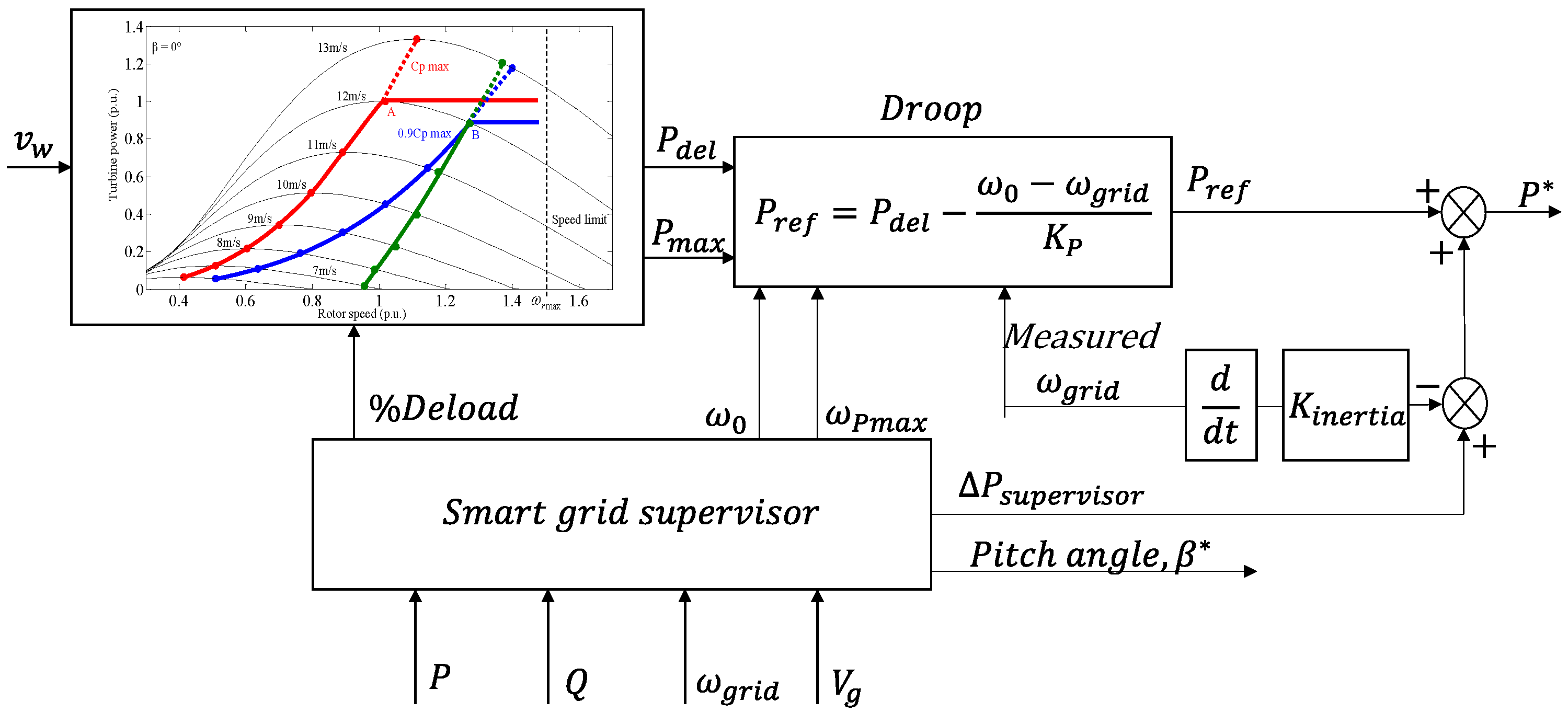
The power of the turbine produced with the Cp coefficient, for a zero pitch angle and for various wind speeds in relation to the speed of the DFIG rotor is illustrated in Figure 7.
With Equations (24) and (22), various turbine power characteristics are determined as illustrated in Figure 7. The red one belongs to the maximum achievable power, in which the power coefficient is the highest available. The blue and green curves are the deloaded power curves. The blue curve represents a 10% deloaded power curve at each given wind speed, being able to extract when necessary a 10% of the maximum power for that wind speed. However, the green curve allows 10% of the maximum power to be extracted at any wind speed. The deload procedure decreases the efficiency of a wind turbine by raising the tip speed ratio. Thus, the deload curves shift to the right of the maximum power curve. Because of the increase in speed, kinetic energy is stored in the inertia of the wind turbine and is expressed as
where is the wind turbine inertia, is the turbine deloaded speed and is the maximum power speed or optimum speed as illustrated in Figure 7. This energy could be employed for short-term frequency control [38]. The additional active power that can be achieved for the deloading operation can be derived from Equation (22) and is dependent on the wind speed and the deloading percentage used as
is the power reserve, is the increase in the power coefficient when the turbine moves from the deloaded working point to a greater power line. This power increase is utilized for long-term frequency adjustment [30].
The reference calculation of the downloaded DFIG speed for every wind speed starts with the specification of the optimal tip speed relation. Thereafter, with the extra active power demanded by the smart grid supervisor, the new tip speed ratio is computed based on Equations (23) and (24).
Observing Figure 7, for 12 m/s of wind speed, the wind turbine can run 10% deloaded as in point B. When the grid frequency decreases, due to a sudden increase in the load, the DFIG must boost the set point of the desired active power. Consequently, the operating power coefficient of the wind turbine moves from the point B of the deloaded curve to the point A of the higher power curve.
In this way, the increase in active power supports the control of the grid frequency. If the highest deloaded power is achieved, (point B) due to increased wind speed, the pitch controller will be required to maintain the required power reserve, which is the difference between the red and blue horizontal lines.
The pitch controller can be used also to avoid overstress or to limit the speed of the wind turbine while regulating the frequency [20].
The major issue of the wind generator is the uncontrollability of the wind as its speed variations affect the amount of energy stored. The manner of saving the desired amount of power, regardless of the wind speed, is to deload the wind turbine for a specified power value as shown in Figure 7. For instance, the green curve shows that the reserved power is 10% of the maximum power for all speeds.
However, working in this way wastes a large amount of wind energy at low speeds. In Figure 8, a diagram is shown for the generation of the active power reference to be introduced in the P* input of the DFIG control scheme presented in Figure 2. Figure 8 also includes droop control, inertial energy, and the pitch controller. The pitch controller will act when the active power surpasses the maximum deloaded power, the peak mechanical power or when the wind turbine speed is greater than the higher limit [39]. The control command is applied by the network supervisor for other control strategies such as automatic control of generation and energy flow or to limit the energy level to a specified level [20,40].
6. Reactive Power and Voltage Amplitude Control
The amplitude of the stator voltage is regulated by adjusting the reactive power as described in the Section 4.
The reactive energy is controlled by the GSC and by the RSC [17]. Both converters are dimensioned to handle about 30% of the nominal power of the generator. Converters are principally utilized to supply the active energy from the rotor to the stator or vice versa. The GSC can be employed to supply reactive energy together with the stator to the grid.
It should be noted that the maximum grid-side converter current cannot be exceeded and therefore the amount of reactive power that can be injected by the grid-side converter will depend on the amount of active power flowing through the rotor. Thus, when the speed of the rotor is synchronous, the active power through the rotor is approximately zero and therefore the reactive power could be maximum. However, as the power through the rotor increases due to an increase in slip, the reactive power must be reduced.
As shown in Equation (12), the reactive power through the stator is regulated by the rotor current d-component. When the load increases suddenly, not only does the frequency decrease, but also the amplitude of the grid voltage tends to be reduced. Because of that, the active and reactive power increases trying to correct the frequency and the amplitude of the grid voltage.
The rotor current must be limited to its maximum value taking into account the active and reactive power values. Equation (27), derived from Equations (11) and (12), provides the maximum active and reactive powers permitted considering the rotor maximum current,
A graphical representation of Equation (27) in Figure 9, illustrates the full range of generation in steady state. If is greater than zero, the DFIG absorbs reactive energy due to its inductive feature [41], however, values lower than zero correspond to the reactive power that the DFIG is able to supply to the grid.
Figure 10 illustrates the red curve of maximum mechanical power that can be obtained for the specified wind speeds. The blue and green curves show the reactive power that the DFIG can provide to the grid when the generator is operating at rated rotor current.
The blue line corresponds to a 1.2 MW DFIG and the green line to a 7.5 kW DFIG. When the DFIG is taking the maximum power of the wind, all the rotor current is formed by the q component and the value of the d component will be zero. This implies that the reactive power is absorbed from the grid and its value will be defined by Equation (12). As shown in the figure, the lower the mechanical power, the more reactive power the DFIG can provide to the grid to compensate for the voltage drop in the grid.
The selection of the maximum active power in the grid frequency compensation does not provide any choice to assist in the correction of the grid amplitude from the stator, but the GSC could be used if their current limit is maintained. This is why certain criteria must be detailed by the smart grid controller in the distribution of the maximum active and reactive powers while respecting the current limits of the stator, rotor and the GSC. Figure 11 provides a diagram for generating the reactive power references of the stator and the GSC converter. The value of depends on the capacity of the DFIG to supply reactive power and this value changes as the active power varies as shown in Figure 10. The control signal is employed by the grid controller for additional regulation strategies, like for example power factor compensation.
7. Experimental Results
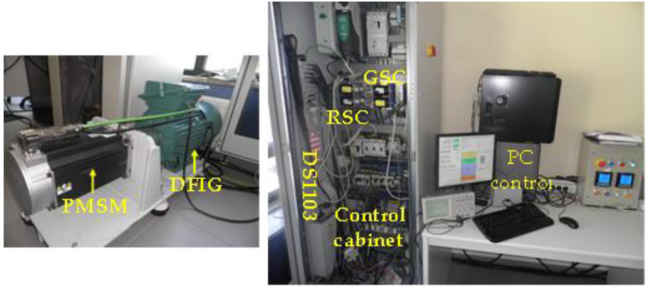
Figure 12 shows the picture of the real test bench for testing the suggested controlling solutions. The system consists of a 7.5 kW DFIM and a 10 kW synchronous machine (PMSM) that performs the tasks of a household wind turbine [42,43,44,45]. The probes for monitoring all the currents and voltages of the system are matched and wired to a DS1103 dSPACE [44] control system.
The gate signals of the RSC and GSC IGBTs are generated by the DS1103 and the rotor position and speed are determined by a 4096 encoder wired to the DS1103. The main characteristics of the double feed induction machine are given in Table 1. The RSC and GSC are two NFS-200 converters with Mitsubishi IGBTs fabricated by Dutt [46]. Three 2 mH @ 15A inductors form the line filter between the GSC and the grid.
Before connecting the DFIM to the grid, the DC bus formed by the RSC and GSC capacitors in a back-to-back configuration must be charged. Once the DC Bus is charged and if the output voltage vector of the GSC is aligned with the grid voltage vector, the GSC connects to the grid and starts the regulation of the DC Bus voltage to a set value of 580 V.
When the wind (emulated by the PMSM) reaches the minimum speed of 5 m/s, the double fed induction machine starts the process of hooking up to the grid. This is done in two stages. In the first stage, the encoder offset with respect to the stator flux must be obtained. In the second stage, the voltage vector generated by the stator must be aligned with the grid voltage vector. When the last process is complete, the DFIM’s stator is connected to the grid and the actual regulation process begins.
Figure 13 shows the regulation of the DFIG when the wind speed changes from 7 to 12 and then to 15 m/s. This means a rotor speed from 900 (sub-synchronous speed) to 1500 (synchronous speed) and then to 1900 rpm (super-synchronous speed) respectively.
In the DFIG the energy from the stator always flows into the grid. The flow of energy via the rotor changes sense depending on the speed of the DFIG. Thus, when the speed of the DFIG is lower than the synchronous speed, the energy of the rotor is absorbed from the grid and goes from the rotor to the stator, in the figure the interval from 0.5 to 1.5 s at 7 m/s of wind speed. Because of this, the total power is inferior to the power of the stator. When the DFIG speed is higher than the synchronous speed, the rotor energy changes sense and goes from the rotor to the grid.
As soon as the total power exceeds the nominal power (7.5 kW) and the wind speed increases, the pitch regulator forces a modification of the pitch angle to ensure that the generator does not exceed the nominal power. As it can be observed in the figure, since no changes are made to the reactive power reference, the d component of the rotor current is constant. However, due to changes in wind speed and therefore in mechanical power, the q component of the rotor changes as does the power of the stator.
Figure 14 shows the implementation made on the real platform to experimentally check the contribution of the DFIG on the voltage amplitude when the load is connected to the grid.
To observe the voltage variation at the PCC (point of common coupling), an inductive load is set where and . The wind speed is fixed to 6 m/s and Figure 15 shows the grid phase voltage amplitude reduction when the load is connected at t = 0.5 s. Due to the inductive characteristic of the line and the inductive load, there is a 5 V reduction in the PCC. At 0.75 s the voltage compensation is activated, supplying the DFIG through the stator with a capacitive reactive power of 7 KVAR (maximum rotor current). This results in a voltage increase on the PCC of 1.5 V. Since the GSC (grid side converter) is able to provide reactive power, 14 KVAR of capacitive reactive power is injected at 1.25 s ordered by the grid supervisor, which causes an additional 3 V increase bringing the PCC voltage closer to the grid voltage.
Due to the impossibility of varying the frequency on the real platform, a simulation is performed to observe the frequency variation on the PCC. The grid is configured so that its frequency varies as a function of the active power consumed, as occurs in a generator. Thus, the grid decreases by 1 Hz when there is an active power consumption of 10 kW. Therefore, in our test the frequency value drops from 50 Hz when there is no consumption to 49 Hz when the consumption in the grid is 10 kW.
If the power is negative (the grid absorbs energy), the frequency increases in the same ratio. The active power is consumed when the load is connected in the line of Figure 14 with a resistive load where and , that is 5.5 kW are consumed for the load.
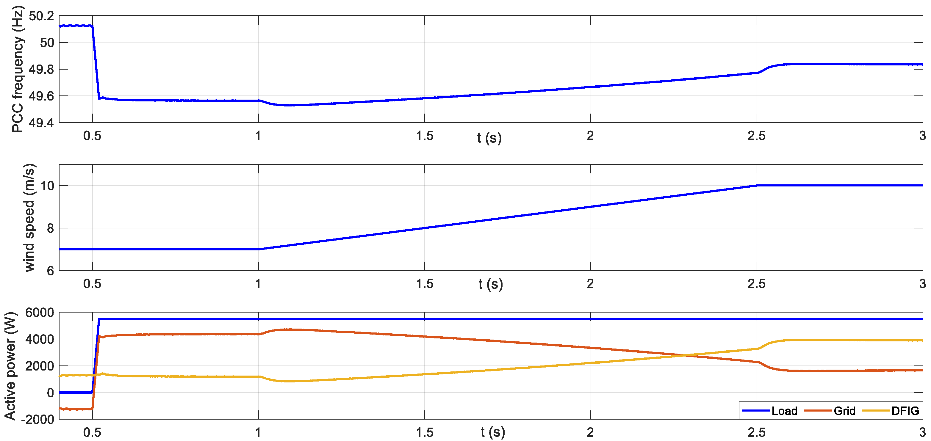
Figure 16 illustrates the behavior of the system by showing the frequency of the PCC, the wind speed and the active powers of the load, the grid and the DFIG. The wind speed has been set at 7 m/s up to 1 s. With this wind the power that the DFIG delivers is 1.5 kW. Up to 0.5 s the grid absorbs this power and the grid frequency at the PCC point is 50.15 Hz. At 0.5 s, the load that absorbs 5.5 kW is connected producing a decrease in frequency of 0.55 Hz, until it reaches 49.6 Hz. From 1 s, the wind speed increases as shown in the figure until it reaches 10 m/s, producing an increase in the contribution of active power to the grid, up to 3.9 kW and reducing the contribution to be made by the grid to 1.6 kW.
This reduction of the active power contribution by the grid means a recovery of the frequency in the grid at 49.83 Hz.
Figure 17 presents the behavior of the system by showing the frequency of the PCC, the power coefficient CP, the DFIG mechanical speed and the active powers of the load, the grid and the DFIG. The wind speed has been set at 12 m/s for all the time. From the beginning the DIFG is running to 2300 rpm, this speed is higher than the optimum speed, thus the DFIG is working 35% deloaded generating 3.5 kW when the obtainable maximum power is 5.4 kW. The load is connected at 0.75 s, which means a drop in frequency from 50.16 to 49.6 Hz. In the instant of 1 s, the energy is extracted from the wind, going from the deloaded working speed to the maximum power speed. This speed deceleration (from 2300 to 1780 rpm) provides extra kinetic energy which produces an increase in frequency until it stabilizes at 49.8 Hz when the maximum possible power is extracted from the wind. Obviously, if it is not possible to extract more energy from the wind it is not possible to reduce the frequency deviation further. The important currents that reflect the process shown in Figure 17, can be seen in Figure 18. In this figure, the grid current, the current consumed by the load, the stator current of the DFIG, the current of the grid side converter and finally the current through the rotor of the DFIG can be seen.
Until 0.75 s the load is disconnected and the DFIG works in deloaded mode. The generator works in super-synchronous speed and the power is delivered to the grid by the stator and the rotor or GSC converter. The generated power of 3.5 kW produces a stator peak current of 4.4 A and a GSC peak current of 1.7 A with the imposed reactive power of 0 VAR. When the load is connected at 0.75 s the power consumption is 5.54 kW and the load peak current is 11.2 A. Since the power delivered by the DFIG is less than the power absorbed by the load, the grid must supply the difference and therefore the grid current peak becomes 5.1 A. In the instant 1 s it passes from the state of deloaded to the point of maximum power. As the deceleration from 2300 to 1780 rpm occurs, the power delivered by the DFIG increases as the CP of the turbine increases and also recovers kinetic energy in deceleration. For this reason, the stator and grid side converter currents increase while the grid current decreases. Finally, when the DFIG reaches full power speed, the current through the stator is 8.4 A and through the GSC is 1.3 A. The rest of the current, until reach the 11.2 A that the load absorbs, is provided by the grid. The amplitude variation of the rotor current is small since the d component of the current predominates to impose a reactive power of 0 VAR. The Ird value is 16.5 A and the amplitude variations are due to the variation of the Irq component to manage the active power. The frequency reduction of the current is observed as it approaches the synchronism speed.
8. Conclusions
This article proposes the use of the double feed induction generator in wind power systems to control the frequency and the amplitude of the point of common coupling voltage. It has been demonstrated that the DFIG must be deloaded to extract the active power from the wind that is required to compensate for the frequency of the grid, and the smart grid controller must establish the quantity deloaded. In addition, the smart grid controller has to choose the required maximum reactive power, taking into account the electrical limits of the double fed induction generator, to balance out the amplitude of the grid voltage. The capacity given to a smart grid to handle frequency and voltage amplitude enhances the reliability of the installation.
The efficiency of the wind turbine is reduced when it is desired to reserve the wind energy in a wind turbine to compensate for the frequency. Since the maximum current value of the DFIG limits the active and reactive power set, by using the converter on the grid side, the reactive power injection can be increased to compensate the grid voltage. Frequency compensation has been tested by performing simulations creating a weak grid. However, the voltage compensation has been implemented in a real platform with a commercial DFIG that has successfully validated the algorithms presented, allowing the commercial implementation of such a system.
Author Contributions
Methodology, J.A.C. and O.B.; Software, O.B., P.A. and J.C.; Hardware and tests, J.A.C., P.A. and J.C. Writing—original draft, J.A.C.; Writing—review editing, O.B., P.A. and J.C. All authors have read and agreed to the published version of the manuscript.
Funding
This research was funded by the Basque Government through the project SMAR3NAK (ELKARTEK KK-2019/00051), the Diputación Foral de Álava (DFA) through the project CONAVAUTIN 2 and the University of the Basque Country (UPV/EHU) through (PPGA20/06).
Institutional Review Board Statement
Not applicable.
Informed Consent Statement
Not applicable.
Data Availability Statement
Not applicable.
Conflicts of Interest
The authors declare no conflict of interest.
Nomenclature
| Rotor side converter | |
| Grid side converter | |
| Direct and quadrature axes expressed in the stationary reference frame | |
| Rotor direct and quadrature axes expressed in the rotor reference frame | |
| Direct and quadrature axes expressed in the synchronous rotating reference frame | |
| Stator voltage vector | |
| Stator current vector | |
| Stator flux vector | |
| Lm | DFIG mutual inductance |
| Ls | DFIG stator inductance |
| Lr | DFIG rotor inductance |
| Lls | DFIG stator leakage inductance |
| Llr | DFIG rotor leakage inductance |
| Rs | DFIG stator resistance |
| Rr | DFIG rotor resistance |
| ωe | Synchronous speed |
| ωr | Rotor electrical speed |
| ωm | Rotor mechanical speed |
| Te | DFIG electromagnetic torque |
| TL | DFIG load torque |
| J | DFIG inertia |
| B | DFIG friction coefficient |
| RL | Load resistance |
| LL | Load inductance |
| Ps | DFIG stator active power |
| Qs | DFIG stator reactive power |
| Pp | Pair of poles |
| Grid voltage vector | |
| Grid current vector | |
| Rg | Grid filter resistance |
| Lg | Grid filter inductance |
| ωg | Grid frequency |
| Grid side converter output voltage vector | |
| Pg | Grid side converter active power |
| Qg | Grid side converter reactive power |
| P | DFIG total active power |
| Q | DFIG total reactive power |
| S | DFIG total apparent power |
| Z | Line impedance |
| KP | Voltage droop coefficient |
| KQ | Frequency droop coefficient |
| Vs | |
| Vg | |
| Angle between the DFIG stator voltage and the grid voltage | |
| Propeller speed | |
| Deloading propeller speed | |
| Propeller optimum speed | |
| Line inductance | |
| IGBT | Insulated gate bipolar transistor |
References and Note
- Future of Wind: Deployment, Investment, Technology, Grid Integration and Socio-Economic Aspects; A Global Energy Transformation Paper; International Renewable Energy Agency (IRENA): Abu Dhabi, UAE, 2019.
- Tasneem, Z.; Al Noman, A.; Das, S.K.; Saha, D.K.; Islam, R.; Ali, F.; Badal, F.R.; Ahamed, H.; Moyeen, S.I.; Alam, F. An analytical review on the evaluation of wind resource and wind turbine for urban application: Prospect and challenges. Dev. Built Environ. 2020, 4, 100033. [Google Scholar] [CrossRef]
- Sunderland, K.M.; Mills, G.; Conlon, M.F. Estimating the wind resource in an urban area: A case study of micro-wind generation potential in Dublin, Ireland. J. Wind Eng. Ind. Aerodyn. 2013, 118, 44–53. [Google Scholar] [CrossRef] [Green Version]
- Drew, D.R.; Barlow, J.F.; Cockerill, T.T. Estimating the potential yield of small wind turbines in urban areas: A case study for Greater London, UK. J. Wind Eng. Ind. Aerodyn. 2013, 115, 104–111. [Google Scholar] [CrossRef] [Green Version]
- Tanvir, A.A.; Merabet, A. Artificial Neural Network and Kalman Filter for Estimation and Control in Standalone Induction Generator Wind Energy DC Microgrid. Energies 2020, 13, 1743. [Google Scholar] [CrossRef] [Green Version]
- Guerrero, J.M.; Lumbreras, C.; Reigosa, D.; Garcia, P.; Briz, F. Control and emulation of small wind turbines using torque estimators. IEEE Trans. Industy Appl. 2011, 53, 4863–4876. [Google Scholar] [CrossRef] [Green Version]
- Calabrese, D.; Tricarico, G.; Brescia, E.; Cascella, G.L.; Monopoli, V.G.; Cupertino, F. Variable Structure Control of a Small Ducted Wind Turbine in the Whole Wind Speed Range Using a Luenberger Observer. Energies 2020, 13, 4647. [Google Scholar] [CrossRef]
- Liu, T.; Gong, A.; Song, C.; Wang, Y. Sliding Mode Control of Active Trailing-Edge Flap Based on Adaptive Reaching Law and Minimum Parameter Learning of Neural Networks. Energies 2020, 13, 1029. [Google Scholar] [CrossRef] [Green Version]
- Bashetty, S.; Guillamon, J.I.; Mutnuri, S.S.; Ozcelik, S. Design of a Robust Adaptive Controller for the Pitch and Torque Control of Wind Turbines. Energies 2020, 13, 1195. [Google Scholar] [CrossRef] [Green Version]
- Kong, X.; Ma, L.; Liu, X.; Abdelbaky, M.A.; Wu, Q. Wind Turbine Control Using Nonlinear Economic Model Predictive Control over All Operating Regions. Energies 2020, 13, 184. [Google Scholar] [CrossRef] [Green Version]
- Elorza, I.; Calleja, C.; Pujana-Arrese, A. On Wind Turbine Power Delta Control. Energies 2019, 12, 2344. [Google Scholar] [CrossRef] [Green Version]
- Barambones, O.; Cortajarena, J.A.; Calvo, I.; Gonzalez de Durana, J.M.; Alkorta, P.; Karami, A. Variable speed wind turbine control scheme using a robust wind torque estimation. Renew. Energy 2018, 133, 354–366. [Google Scholar] [CrossRef]
- Hansen, A.D.; Iov, F.; Blaabjerg, F.; Hansen, L.H. Review of contemporary wind turbine concepts and their market penetration. J. Wind Eng. 2004, 28, 247–263. [Google Scholar] [CrossRef]
- Ananth, D.V.N.; Nagesh Kumar, G.V. Tip Speed Ratio Based MPPT Algorithm and Improved Field Oriented Control for Extracting Optimal Real Power and Independent Reactive Power Control for Grid Connected Doubly Fed Induction Generator. Int. J. Electr. Comput. Eng. 2016, 6, 1319–1331. [Google Scholar]
- Amrane, F.; Chaiba, A.; Francois, B.; Babes, B. Experimental design of stand-alone field oriented control for WECS in variable speed DFIG-based on hysteresis current controller. In Proceedings of the 2017 15th International Conference on Electrical Machines, Drives and Power Systems, Sofia, Bulgaria, 1–3 June 2017; pp. 1–5. [Google Scholar]
- Djilali, L.; Sanchez, E.N.; Belkheir, M. Real-time implementation of sliding-mode field-oriented control for a DFIG-based wind turbine. Int. Trans. Electr. Energy Syst. 2018, 28, e2539. [Google Scholar] [CrossRef]
- Kaloi, G.S.; Wang, J.; Baloch, M.H. Active and reactive power control of the doubly fed induction generator based on wind energy conversion system. Energy Rep. 2016, 2, 194–200. [Google Scholar] [CrossRef] [Green Version]
- Soued, S.; Ramadan, H.S.; Becherif, M. Dynamic Behavior Analysis for Optimally Tuned On-Grid DFIG Systems. Special Issue on Emerging and Renewable Energy: Generation and Automation. ScienceDirect. Energy Procedia 2019, 162, 339–348. [Google Scholar] [CrossRef]
- Shenglong, Y.; Kianoush, E.; Tyrone, F.; Herbert, H.C.J.; Kit, P.W. State Estimation of Doubly Fed Induction Generator Wind Turbine in Complex Power Systems. IEEE Trans. Power Syst. 2016, 31, 4935–4944. [Google Scholar]
- Palensky, P.; Dietrich, D. Demand side management: Demand response, intelligent energy systems and smart loads. IEEE Trans. Ind. Inform. 2011, 7, 381–389. [Google Scholar] [CrossRef] [Green Version]
- Güngör, V.C.; Sahin, D.; Kocak, T.; Ergüt, S.; Buccella, C.; Cecati, C.; Hancke, G.P. Smart grid technologies: Communication technologies and standards. IEEE Trans. Ind. Inform. 2011, 7, 529–539. [Google Scholar] [CrossRef] [Green Version]
- Zhang, Y.; Meng, F.; Wang, R.; Kazemtabrizi, B.; Shi, J. Uncertainty-resistant stochastic MPC approach for optimal operation of CHP microgrid. Energy 2019, 179, 1265–1278. [Google Scholar] [CrossRef]
- Nguyen, T.T.; Yoo, H.J.; Kim, H.M. Analyzing the Impacts of System Parameters on MPC-Based Frequency Control for a Stand-Alone Microgrid. Energies 2017, 10, 417. [Google Scholar] [CrossRef] [Green Version]
- Bayhan, H.A.; Ellabban, O. Sensorless model predictive control scheme of wind-driven doubly fed induction generator in dc microgrid. IET Renew. Power Gener. 2016, 10, 514–521. [Google Scholar] [CrossRef]
- Valencia-Rivera, G.H.; Merchan-Villalba, L.R.; Tapia-Tinoco, G.; Lozano-Garcia, J.M.; Avina-Cervantes MA, I.M.; Gabriel, J. Hybrid LQR-PI Control for Microgrids under Unbalanced Linear and Nonlinear Loads. Mathematics 2020, 8, 1096. [Google Scholar] [CrossRef]
- Thounthong, P.; Mungporn, P.; Pierfederici, S.; Guilbert, D.; Bizon, N. Adaptive Control of Fuel Cell Converter Based on a New Hamiltonian Energy Function for Stabilizing the DC Bus in DC Microgrid Applications. Mathematics 2020, 8, 2035. [Google Scholar] [CrossRef]
- Qiao, W.; Harley, R.G. Grid Connection Requirements and Solutions for DFIG Wind Turbines; IEEE: Piscataway, NJ, USA, 2008. [Google Scholar]
- Cortajarena, J.A.; De Marcos, J.; Alkorta, P.; Barambones, O.; Cortajarena, J. DFIG wind turbine grid connected for frequency and amplitude control in a smart grid. In Proceedings of the 2018 IEEE International Conference on Industrial Electronics for Sustainable Energy Systems (IESES), Hamilton, New Zealand, 31 January–2 February 2018. [Google Scholar]
- Li, S.; Challoo, R.; Nemmers, M.J. Comparative Study of DFIG Power Control Using Stator Voltage and Stator-Flux Oriented Frames. In Proceedings of the 2009 IEEE Power & Energy Society General Meeting, Calgary, AB, Canada, 26–30 July 2009; pp. 1–8. [Google Scholar]
- Ghosh, S.; Isbeih, Y.J.; Bhattarai, R.; El Moursi, M.S.; El-Saadany, E.F. A Dynamic Coordination Control Architecture for Reactive Power Capability Enhancement of the DFIG-Based Wind Power Generation. IEEE Trans. Power Syst. 2020, 35, 3051–3064. [Google Scholar] [CrossRef]
- Cortajarena, J.A.; Barambones, O.; Alkorta, P.; De Marcos, J. Sliding mode control of grid-tied single-phase inverter in a photovoltaic MPPT application. Solar Energy 2017, 155, 793–804. [Google Scholar] [CrossRef]
- Kazmierkowski, M.P.; Jasinski, M.; Wrona, G. DSP-Based control of grid-connected power converters operating under grid distortions. IEEE Trans. Ind. Inform. 2011, 7, 204–211. [Google Scholar] [CrossRef]
- Guerrero, J.M.; Matas, J.; Vicuña, L.G.; Castilla, M.; Miret, J. Decentralized control for parallel operation of distributed generation inverters using resistive output impedance. IEEE Trans. Ind. Electron. 2007, 54, 994–1004. [Google Scholar] [CrossRef]
- Guerrero, J.M.; Vicuña, L.G.; Matas, J.; Castilla, M.; Miret, J. A wireless controller to enhance dynamic performance of parallel inverters in distributed generation systems. IEEE Trans. Power Electron. 2004, 19, 1205–1213. [Google Scholar] [CrossRef]
- Mun-Kyeom, K. Optimal Control and Operation Strategy for Wind Turbines Contributing to Grid Primary Frequency Regulation. Appl. Sci. 2017, 7, 1–23. [Google Scholar]
- Aho, J.; Buckspan, A.; Laks, J.; Fleming, P.; Jeong, Y.; Dunne, F.; Churchfield, M.; Pao, L.; Johnson, K. Tutorial of Wind Turbine Control for Supporting Grid Frequency through Active Power Control. In Proceedings of the 2012 American Control Conference (ACC), Montréal, QC, Canada, 27–29 June 2012; pp. 1–12. [Google Scholar]
- Matlab/Simulink. Wind turbine model. 2009.
- Ramtharan, G.; Ekanayake, J.B.; Jenkins, N. Frequency support from doubly fed induction generator wind turbines. IET Renew. Power Gener. 2007, 1, 3–9. [Google Scholar] [CrossRef]
- Saenz-Aguirre, A.; Zulueta, E.; Fernandez-Gamiz, U.; Teso-Fz-Betoño, D.; Olarte, J. Kharitonov Theorem Based Robust Stability Analysis of a Wind Turbine Pitch Control System. Mathematics 2020, 8, 964. [Google Scholar] [CrossRef]
- North American Electric Reliability Corporation. Accommodating High Levels of Variable Generation; North American Electric Reliability Corporation: Princeton, NJ, USA, 2009. [Google Scholar]
- Kayikc, M.; Milanovic, J.V. Reactive power control strategies for DFIG-based plants. IEEE Trans. Energy Convers. 2007, 22, 389–396. [Google Scholar]
- Gallardo, S.; Carrasco, J.M.; Galván, E.; Franquelo, L.G. DSP-based doubly fed induction generator test bench using a back-to-back PWM converter. In Proceedings of the 2004 30th Annual Conference of the IEEE Industrial Electronics Society, Busan, Korea, 2–6 November 2004. [Google Scholar]
- dSPACE. Real–Time Interface. In Implementation Guide. Experiment Guide; For Realese 5.0.; GmbH: Paderborn, Germany, 2005. [Google Scholar]
- Cortajarena, J.A.; De Marcos, J.; Alvarez, P.; Vicandi, F.J.; Alkorta, P. Start up and control of a DFIG wind turbine test rig. In Proceedings of the 2011 37th Annual Conference of the IEEE Industrial Electronics Society, Melbourne, VIC, Australia, 7–10 November 2011. [Google Scholar]
- Junseon, P.; Seungjin, L.; Joong Yull, P. Effects of the Angled Blades of Extremely Small Wind Turbines on Energy Harvesting Performance. Mathematics 2020, 8, 1295. [Google Scholar]
- Dutt. Power Electronics & Control. Available online: http://www.duttelectronics.com (accessed on 2 October 2020).
Figure 1.
DFIG reference systems.

Figure 2.
DFIG control structure.

Figure 3.
Grid voltage reference system.

Figure 4.
Grid side converter control structure.

Figure 5.
DFIG generator connected to the main grid trough line impedance.

Figure 6.
Droop characteristics. Left frequency, right voltage.

Figure 7.
Turbine deloaded and maximum power curves.

Figure 8.
DFIG reference generation of active power. Droop and smart grid supervisor defined control.
Figure 8.
DFIG reference generation of active power. Droop and smart grid supervisor defined control.

Figure 9.
Stator boundaries for rated current of the rotor.

Figure 10.
Maximum mechanical power and reactive powers obtainable for maximum rotor current. DFIG 7.5 kW, green curve. DFIG 1.2 MW, blue curve.
Figure 10.
Maximum mechanical power and reactive powers obtainable for maximum rotor current. DFIG 7.5 kW, green curve. DFIG 1.2 MW, blue curve.

Figure 11.
Diagram for generating the reactive power references of the stator and the GSC converter.
Figure 11.
Diagram for generating the reactive power references of the stator and the GSC converter.

Figure 12.
DFIG platform used to test the proposed control strategies.

Figure 13.
DFIG signals for a wind speed from 7 to 15 m/s. Upper graph, wind speed reference. Second graph, stator, rotor, turbine and total electrical power. Third graph, pitch angle. Fourth graph, references and actual values of rotor current d and q components.
Figure 13.
DFIG signals for a wind speed from 7 to 15 m/s. Upper graph, wind speed reference. Second graph, stator, rotor, turbine and total electrical power. Third graph, pitch angle. Fourth graph, references and actual values of rotor current d and q components.

Figure 14.
Single line diagram of the system implemented and used for testing.

Figure 15.
Load voltage for inductive load and voltage compensation with the controlled DFIG reactive power for Figure 14 structure.
Figure 15.
Load voltage for inductive load and voltage compensation with the controlled DFIG reactive power for Figure 14 structure.

Figure 16.
PCC frequency, wind speed and active power. Frequency drop compensation for the resistive load in the scheme of Figure 14.
Figure 16.
PCC frequency, wind speed and active power. Frequency drop compensation for the resistive load in the scheme of Figure 14.

Figure 17.
PCC frequency, CP coefficient, DFIG speed, and active power. Frequency drop compensation for the resistive load in the scheme in Figure 14 with the DFIG working deloaded.
Figure 17.
PCC frequency, CP coefficient, DFIG speed, and active power. Frequency drop compensation for the resistive load in the scheme in Figure 14 with the DFIG working deloaded.

Figure 18.
Grid, load, stator, grid side converter, and rotor currents for the process shown in Figure 17.
Figure 18.
Grid, load, stator, grid side converter, and rotor currents for the process shown in Figure 17.


Table 1.
Leroy Somer DFIM main parameters
| Parameter | Value |
|---|---|
| Stator voltage | 380 V |
| Rotor voltage | 190 V |
| Rated stator current | 18 A |
| Rated rotor current | 24 A |
| Rated speed | 1447 rpm @ 50 Hz |
| Rated torque | 50 Nm |
| Stator resistance | 0.325 Ω |
| Rotor resistance | 0.275 Ω |
| Magnetizing inductance | 0.0664 H |
| Stator leakage inductance | 0.00264 H |
| Rotor leakage inductance | 0.00372 H |
| Inertia moment | 0.07 Kg*m2 |
Publisher’s Note: MDPI stays neutral with regard to jurisdictional claims in published maps and institutional affiliations. |
© 2021 by the authors. Licensee MDPI, Basel, Switzerland. This article is an open access article distributed under the terms and conditions of the Creative Commons Attribution (CC BY) license (http://creativecommons.org/licenses/by/4.0/).
Share and Cite
MDPI and ACS Style
Cortajarena, J.A.; Barambones, O.; Alkorta, P.; Cortajarena, J. Grid Frequency and Amplitude Control Using DFIG Wind Turbines in a Smart Grid. Mathematics 2021, 9, 143. https://doi.org/10.3390/math9020143
AMA Style
Cortajarena JA, Barambones O, Alkorta P, Cortajarena J. Grid Frequency and Amplitude Control Using DFIG Wind Turbines in a Smart Grid. Mathematics. 2021; 9(2):143. https://doi.org/10.3390/math9020143
Chicago/Turabian StyleCortajarena, José Antonio, Oscar Barambones, Patxi Alkorta, and Jon Cortajarena. 2021. "Grid Frequency and Amplitude Control Using DFIG Wind Turbines in a Smart Grid" Mathematics 9, no. 2: 143. https://doi.org/10.3390/math9020143
Note that from the first issue of 2016, this journal uses article numbers instead of page numbers. See further details here.