
A Block Coordinate Descent-Based Projected Gradient Algorithm for Orthogonal Non-Negative Matrix Factorization


1
Institute for Data Science, School of Engineering, University of Applied Sciences and Arts Northwestern Switzerland, 5210 Windisch, Switzerland
2
Faculty of Mechanical Engineering, University of Ljubljana, Aškerčeva ulica 6, SI-1000 Ljubljana, Slovenia
3
Institute of Mathematics, Physics and Mechanics, Jadranska 19, SI-1000 Ljubljana, Slovenia
*
Author to whom correspondence should be addressed.
Mathematics 2021, 9(5), 540; https://doi.org/10.3390/math9050540
Submission received: 8 December 2020
/
Revised: 15 February 2021
/
Accepted: 24 February 2021
/
Published: 4 March 2021
(This article belongs to the Section Mathematics and Computer Science)
Abstract
:This article uses the projected gradient method (PG) for a non-negative matrix factorization problem (NMF), where one or both matrix factors must have orthonormal columns or rows. We penalize the orthonormality constraints and apply the PG method via a block coordinate descent approach. This means that at a certain time one matrix factor is fixed and the other is updated by moving along the steepest descent direction computed from the penalized objective function and projecting onto the space of non-negative matrices. Our method is tested on two sets of synthetic data for various values of penalty parameters. The performance is compared to the well-known multiplicative update (MU) method from Ding (2006), and with a modified global convergent variant of the MU algorithm recently proposed by Mirzal (2014). We provide extensive numerical results coupled with appropriate visualizations, which demonstrate that our method is very competitive and usually outperforms the other two methods.
1. Introduction
1.1. Motivation
Many machine learning applications require processing large and high dimensional data. The data could be images, videos, kernel matrices, spectral graphs, etc., represented as an matrix R. The data size and the amount of redundancy increase rapidly when m and n grow. To make the analysis and the interpretation easier, it is favorable to obtain compact and concise low rank approximation of the original data R. This low-rank approximation is known to be very efficient in a wide range of applications, such as: text mining [1,2,3], document classification [4], clustering [5,6], spectral data analysis [1,7], face recognition [8], and many more.
There exist many different low rank approximation methods. For instance, two well-known strategies, broadly used for data analysis, are singular value decomposition (SVD) [9] and principle component analysis (PCA) [10]. Much of real-world data are non-negative, and the related hidden parts express physical features only when the non-negativity holds. The factorizing matrices in SVD or PCA can have negative entries, making it hard or impossible to put a physical interpretation on them. Non-negative matrix factorization was introduced as an attempt to overcome this drawback, i.e., to provide the desired low rank non-negative matrix factors.
1.2. Problem Formulation
A non-negative matrix factorization problem (NMF) is a problem of factorizing the input non-negative matrix R into the product of two lower rank non-negative matrices G and H:
where usually corresponds to the data matrix, represents the basis matrix, and is the coefficient matrix. With p we denote the number of factors for which it is desired that . If we consider each of the n columns of R being a sample of m-dimensional vector data, the factorization represents each instance (column) as a non-negative linear combination of the columns of G, where the coefficients correspond to the columns of H. The columns of G can be therefore interpreted as the p pieces that constitute the data R. To compute G and H, condition (1) is usually rewritten as a minimization problem using the Frobenius norm:
It is demonstrated in certain applications that the performance of the standard NMF in (NMF) can often be improved by adding auxiliary constraints which could be sparseness, smoothness, and orthogonality. Orthogonal NMF (ONMF) was introduced by Ding et al. [11]. To improve the clustering capability of the standard NMF, they imposed orthogonality constraints on columns of G or on rows of H. Considering the orthogonality on columns of G, it is formulated as follows:
If we enforce orthogonality on the columns of G and on rows of H, we obtain the bi-orthogonal ONMF (bi-ONMF), which is formulated as
where I denotes the identity matrix.
While the classic non-negative matrix factorization problem (NMF) has achieved a great attention in the recent decade, see also the recent book [12], and several methods have been devised to compute approximate optimal solutions, the problems with the orthogonality constraints (ONMF)–(bi-ONMF) were much less studied and the list of available methods is much shorter. Most of them are related to the fixed point method and to some variant of update rules. Especially meeting both orthogonality constraints in (bi-ONMF), which is relevant for co-clustering of the data, is still challenging and very limited research has been done in this direction, especially with methods that are not related to the fixed point method approach.
1.3. Related Work
The NMF was firstly studied by Paatero et al. [13,14] and was made popular by Lee and Seung [15,16]. There are several different existing methods to solve (NMF). The most used approach to minimize (NMF) is a simple MU method proposed by Lee and Seung [15,16]. In Chu et al. [17], several gradient-type approaches have been mentioned. Chu et al., reformulated (NMF) as an unconstrained optimization problem, and then applied the standard gradient descent method. Considering both G and H as variables in (NMF), it is obvious that is a non-convex function. However, considering G and H separately, we can find two convex sub-problems. Accordingly, a block-coordinate descent (BCD) approach [16] is applied to obtain values for G and H that correspond to a local minimum of . Generally, the scheme adopted by BCD algorithms is to recurrently update blocks of variables only, while the remaining variables are fixed. NMF methods which adopt this optimization technique are, e.g., the MU rule [15], the active-set-like method [18], or the PG method for NMF [19]. In [19], two PG methods were proposed for the standard NMF. The first one is an alternating least squares (ALS) method using projected gradients. This way, H is fixed first and a new G is obtained by PG. Then, with the fixed G at the new value, the PG method looks for a new H. The objective function in each least squares problem is quadratic. This enabled the author to use Taylor’s extension of the objective function to obtain an equivalent condition with the Armijo rule, while checking the sufficient decrease of the objective function as a termination criterion in a step-size selection procedure. The other method proposed in [19] is a direct application of the PG method to (NMF). There is also a hierarchical ALS method for NMF which was originally proposed in [20,21] as an improvement to the ALS method. It consists of a BCD method with single component vectors as coordinate blocks.
As the original ONMF algorithms in [5,6] and their variants [22,23,24] are all based on the MU rule, there has been no convergence guarantee for these algorithms. For example, Ding et al. [11] only prove that the successive updates of the orthogonal factors will converge to a local minimum of the problem. Because the orthogonality constraints cannot be rewritten into a non-negatively constrained ALS framework, convergent algorithms for the standard NMF (e.g., see [19,25,26,27]) cannot be used for solving the ONMF problems. Thus, no convergent algorithm was available for ONMF until recently. Mirzal [28] developed a convergent algorithm for ONMF. The proposed algorithm was designed by generalizing the work of Lin [29] in which a convergent algorithm was provided for the standard NMF based on a modified version of the additive update (AU) technique of Lee [16]. Mirzal [28] provides the global convergence for his algorithm solving the ONMF problem. In fact, he first proves the non-increasing property of the objective function evaluated by the sequence of the iterates. Secondly, he shows that every limit point of the generated sequence is a stationary point, and finally he proves that the sequence of the iterates possesses a limit point. In more recent literature, NMF is used in very applicative areas. In [30], a procedure for mining biologically meaningful biomarkers from microarray datasets of different tumor histotypes is illustrated. The proposed methodology allows automatically identifying a subset of potentially informative genes from microarray data matrices, which differs either in the number of rows (genes) and columns (patients). The methodology integrates NMF to allow the analysis of omics input data with different row size. In [31], the authors propose the correntropy-based orthogonal nonnegative matrix tri-factorization algorithm, which is robust to noisy data contaminated by non-Gaussian noise and outliers. In contrast to previous NMF algorithms, this algorithm firstly applies correntropy, which is defined as a measure of similarity between two random variables, to non-negative matrix tri-factorization problem to measure the similarity, and preserves double orthogonality conditions and dual graph regularization. Then, they adapt the half-quadratic technique which is based on conjugate function theory to solve the resulting optimization problem, and derive the multiplicative update rules. In [32], the blind audio source separation problem which consists of isolating and extracting each of the sources is studied. To perform this task, the authors use NMF based on the Kullback-Leibler and Itakura-Saito -divergences as a standard technique that itself uses the time-frequency representation of the signal. The new NMF model is based on the minimization of -divergences along with a penalty term that promotes the columns of the dictionary matrix to have a small volume. In [33], the authors use NMF to analyze microarray data which are a kind of numerical non-negative data used to collect gene expression profiles. Since the number of genes in DNA is huge, they are usually high dimensional, therefore they require dimensionality reduction and clustering techniques to extract useful information. The authors use NMF for dimensionality reduction to simplify the data and the relations in the data. To improve the sparseness of the base matrix in incremental NMF, the authors of [34] present a new method, orthogonal incremental NMF algorithm, which combines the orthogonality constraint with incremental learning. This approach adopts batch update in the process of incremental learning.
1.4. Our Contribution
In this paper, we consider the penalty reformulation of (bi-ONMF), i.e., we add the orthogonality constraints multiplied with penalty parameters to the objective function to obtain reformulated problems (ONMF) and (bi-ONMF). The main contributions are:
- We develop an algorithm for (ONMF) and (bi-ONMF), which is essentially a BCD algorithm, in the literature also known as alternating minimization, coordinate relaxation, the Gauss-Seidel method, subspace correction, domain decomposition, etc., see e.g., [35,36]. For each block optimization, we use a PG method and Armijo rule to find a suitable step-size.
- We construct synthetic data sets of instances for (ONMF) and (bi-ONMF), for which we know the optimum value by construction.
- The implemented algorithms are compared on the constructed synthetic data-sets in terms of: (i) the accuracy of the reconstruction, and (ii) the deviation of the factors from the orthonormality. This deviation is a measure the feasibility of the obtained solution and has not been analyzed in the work Of Ding [11] and Mirzal [28]. Accuracy is measured by the so-called root-square error (RSE), defined asPlease note that we added 1 to the denominator in the formula above to prevent numerical difficulties when the data matrix R has a very small Frobenius norm.Deviations from the orthonormality are computed using Formulas (17) and (18) from Section 4. Our numerical results show that our algorithm is very competitive and almost always outperforms the MU based algorithms.
1.5. Notations
Some notations used throughout our work are described here. We denote scalars and indices by lower-case Latin letters, vectors by lowercase boldface Latin letters, and matrices by capital Latin letters. denotes the set of m by n real matrices, and I symbolizes the identity matrix. We use the notation ∇ to show the gradient of a real-valued function. We define and as the positive and (unsigned) negative parts of ∇, respectively, i.e., . ⊙ and ⊘ denote the element-wise multiplication and the element-wise division, respectively.
1.6. Structure of the Paper
The rest of our work is organized as follows. In Section 2, we review the well-known MU method and the rules being used for updating the factors per iteration in our computations. We also outline the global convergent MU version of Mirzal [28]. We then present our PG method and discuss the stopping criteria for it. Section 4 presents the synthetic data and the result of implementation of the three decomposition methods presented in Section 3. This implementation is done for both the problem (ONMF), as well as (bi-ONMF). Some concluding results are presented in Section 5.
2. Existing Methods to Solve (NMF)
2.1. The Method of Ding
Several popular approaches to solve (NMF) are based on so-called MU algorithms, which are simple to implement and often yield good results. The MU algorithms originate from the work of Lee and Seung [16]. Various MU variants were later proposed by several researchers, for an overview see [38]. At each iteration of these methods, the elements of G and H are multiplied by certain updating factors.
As already mentioned, (ONMF) was proposed by Ding et al. [11] as a tool to improve the clustering capability of the associated optimization approaches. To adapt the MU algorithm for this problem, they employed standard Lagrangian techniques: they introduced the Lagrangian multiplier (a symmetric matrix of size ) for the orthogonality constraint, and minimized the Lagrangian function where the orthogonality constraint is moved to the objective function as the penalty term . The complementarity conditions from the related KKT conditions can be rewritten as a fixed point relation, which finally can lead to the following MU rule for (ONMF):
They extended this approach to non-negative three factor factorization with demand that two factors satisfy orthogonality conditions, which is a generalization of (bi-ONMF). The MU rules (28)–(30) from [11], adapted to (bi-ONMF), are the main ingredients of Algorithm 1, which we will call Ding’s algorithm.
| Algorithm 1: Ding’s MU algorithm for (bi-ONMF). |
| INPUT: , |
| 1. Initialize: generate as an random matrix and as a random matrix. |
| 2. Repeat |
| 3. Until convergence or a maximum number of iterations or maximum time is reached. |
| OUTPUT:. |
Algorithm 1 converges in the sense that the solution pairs G and H generated by this algorithm yield a sequence of decreasing RSEs, see [11], Theorems 5 and 7.
If R has zero vector as columns or rows, a division by zero may occur. In contrast, denominators close to zero may still cause numerical problems. To escape this situation, we follow [39] and add a small positive number to the denominators of the MU terms (4). Pleas note that Algorithm 1 can be easily adapted to solve (ONMF) by replacing the second MU rule from (4) with the second MU rule of (3).
2.2. The Method of Mirzal
In [28], Mirzal proposed an algorithm for (ONMF) which is designed by generalizing the work of Lin [29]. Mirzal used the so-called modified additive update rule (the MAU rule), where the updated term is added to the current value for each of the factors. This additive rule has been used by Lin in [29] in the context of a standard NMF. He also provided in his paper a convergence proof, stating that the iterates generated by his algorithm converge in the sense that RSE is decreasing and the limit point is a stationary point. In [28], Mirzal discussed the orthogonality constraint on the rows of H, while in [40] the same results are developed for the case of (bi-ONMF).
Here we review the Mirzal’s algorithm for (bi-ONMF), presented in the unpublished paper [40]. This algorithm actually solves the equivalent problem (pen-ONMF) where the orthogonality constraints are moved into the objective function (the so-called penalty approach), and the importance of the orthogonality constraints are controlled by the penalty parameters :
The gradients of the objective function with respect to G and H are:
For the objective function in (pen-ONMF), Mirzal proposed the MAU rules along with the use of and , instead of G and H, to avoid the zero locking phenomenon [28], Section 2:
where is a small positive number.
Please note that the algorithms working with the MU rules for (pen-ONMF) must be initialized with positive matrices to avoid zero locking from the start, but non-negative matrices can be used to initialize the algorithm working with the MAU rules (see [40]).
Mirzal [40] used the MAU rules with some modifications by considering and in order to guarantee the non-increasing property, with a constant step to make and grow in order to satisfy the property. Here, and are the values added within the MAU terms to the denominator of update terms for G and H, respectively. The proposed algorithm by Mirzal [40] is summarised as Algorithm 2 below.
| Algorithm 2: Mirzal’s algorithm for bi-ONMF [40] |
| INPUT: inner dimension p, maximum number of iterations: maxit; small positive , small positive to increase . |
| 1. Compute initial and . |
| 2. For |
| ; |
| Repeat |
| ; |
| ; |
| Until |
| ; |
| Repeat |
| ; |
| ; |
| Until |
| ; |
| OUTPUT: . |
3. PG Method for (ONMF) and (bi-ONMF)
3.1. Main Steps of PG Method
In this subsection we adapt the PG method proposed by Lin [19] to solve both (ONMF) as well as (bi-ONMF). Lin applied PG to (NMF) in two ways. The first approach is actually a BCD method. This method consecutively fixes one block of variables (G or H) and minimizes the simplified problem in the other variable. The second approach by Lin directly minimizes (NMF). Lin’s main focus was on the first approach and we follow it. We again try to solve the penalized version of the problem (pen-ONMF) by the block coordinate descent method, which is summarised in Algorithm 3.
| Algorithm 3: BCD method for (pen-ONMF) |
| INPUT: inner dimension p, initial matrices . |
| 1. Set . |
| 2. Repeat |
| Fix and compute new G as follows: |
| Fix and compute new H as follows: |
| 3. Until some stopping criteria is satisfied |
| OUTPUT: . |
The objective function in (pen-ONMF) is not quadratic any more, so we lose the nice properties about Armijo’s rule that represent advantages for Lin. We managed to use the Armijo rule directly and still obtained good numerical results, see Section 4. Armijo [41] was the first to establish convergence to stationary points of smooth functions using an inexact line search with a simple “sufficient decrease” condition. The Armijo condition ensures that the line search step is not too large.
We refer to (8) or (9) as sub-problems. Obviously, solving these sub-problems in every iteration could be more costly than Algorithms 1 and 2. Therefore, we must find effective methods for solving these sub-problems. Similarly to Lin, we apply the PG method to solve the sub-problems (8) and (9). Algorithm 4 contains the main steps of the PG method for solving the latter and can be straightforwardly adapted for the former.
For the sake of simplicity, we denote by the function that we optimize in (8), which is actually a simplified version (pure H terms removed) of the objective function from (pen-ONMF) for H fixed:
Similarly, for G is fixed, the objective function from (9) will be denoted by:
In Algorithm 4, P is the projection operator which projects the new point (matrix) on the cone of non-negative matrices (we simply put negative entries to 0).
Inequality (10) shows the Armijo rule to find a suitable step-size guaranteeing a sufficient decrease. Searching for is a time-consuming operation, therefore we strive to do only a small number of trials for new in Step 3.1.
Similarly to Lin [19], we allow for any positive value. More precisely, we start with and if the Armijo rule (10) is satisfied, we increase the value of by dividing it with . We repeat this until (10) is no longer satisfied or the same matrix as in the previous iteration is obtained. If the starting does not yield which would satisfy the Armijo rule (10), then we decrease it by a factor and repeat this until (10) is satisfied. The numerical results obtained using different values of parameters (updating factor for ) and (parameter to check (10)) are reported in the following subsections.
| Algorithm 4: PG method using Armijo rule to solve sub-problem (9) |
| INPUT: , and initial . |
| 1. Set |
| 2. Repeat |
| Find a (using updating factor ) such that for |
| we have |
| Set |
| Set ; |
| 3. Until some stopping criteria is satisfied. |
| OUTPUT: . |
3.2. Stopping Criteria for Algorithms 3 and 4
As practiced in the literature (e.g., see [42]), in a constrained optimization problem with the non-negativity constraint on the variable x, a common condition to check whether a point is close to a stationary point is
where f is the differentiable function that we try to optimize and is the projected gradient defined as
and is a small positive tolerance. For Algorithm 3, (11) becomes
We impose a time limit in seconds and a maximum number of iterations for Algorithm 4 as well. Following [19], we also define stopping conditions for the sub-problems. The matrices and returned by Algorithm 4, respectively, must satisfy
where
and is the same tolerance used in (13). If the PG method for solving the sub-problem (8) or (9) stops after the first iteration, then we decrease the stopping tolerance as follows:
where is a constant smaller then 1.
4. Numerical Results
In this section we demonstrate, how the PG method described in Section 3, performs compared to the MU-based algorithms of Ding and Mirzal, which were described in Section 2.1 and Section 2.2, respectively.
4.1. Artificial Data
We created three sets of synthetic data using MATLAB [37]. The first set we call bi-orthonormal set (BION). It consists of instances of matrix , which were created as products of G and H, where has orthonormal columns while has orthonormal rows. We created five instances of R, for each pair and from Table 1.
Matrices G were created in two phases: firstly, we randomly (uniform distribution) selected a position in each row; secondly, we selected a random number from (uniform distribution) for the selected position in each row. Finally, if it happens that after this procedure some column of G is zero or has a norm below , we find the first non-zero element in the largest column of G (according to Euclidean norm) and move it into the zero column. Then we normalized the columns of G. We created H similarly.
Each triple was saved as a triple of txt files. For example, NMF_BIOG_data_R_n=200_k=80_id=5.txt contains matrix R obtained by multiplying matrices and , which were generated as explained above. With id=5, we denote that this is a 5th matrix corresponding to this pair .
The second set contains similar data to BION, but only one factor (G) is orthonormal, while the other (H) is non-negative but not necessarily orthonormal. We call this dataset uni-orthonormal (UNION).
The third data set is a nosy variant of the first data set. For each triple from the BION data, we computed a new nosy , where E is a random matrix of the same size as R, with entries uniformly distributed on . Parameter is defined such that the expected value of RSE satisfies:
where is parameter chosen by us and was set to . By using basic properties of the uniform distribution, we can easily derive that , where n is the order of square matrix R. We indeed used the right hand side term of this inequality to generate the noise matrices E.
All computations are done using MATLAB [37] and a high performance computer available at Faculty of Mechanical Engineering of University of Ljubljana. This is Intel Xeon X5670 (1536 hyper-cores) HPC cluster and an E5-2680 V3 (1008 hyper-cores) DP cluster, with an IB QDR interconnection, 164 TB of LUSTRE storage, 4.6 TB RAM and with 24 TFlop/s performance.
4.2. Numerical Results for UNION
In this subsection, we present numerical results, obtained by Ding’s, Mirzal’s, and our algorithm for a uni-orthogonal problem (ONMF), using the UNION data, introduced in the previous subsection. We adapted the last two algorithms (Algorithms 2 and 3) for UNION data by setting in the problem formulation (bi-ONMF) and in all formulas underlying these two algorithms.
The maximum number of outer iterations for all three algorithms was set to 1000. In practices, we stop Algorithms 1 and 3 only when the maximum number of iterations is reached, while for Algorithm 2, the stopping condition involved also checking the progress of RSE. If this is too small (below ) we also stop.
Recall that for UNION data we have for each pair from Table 1 five symmetric matrices R for which we try to solve (ONMF) by Algorithms 1–3. Please note that all these algorithms demand as input the internal dimension k, i.e., the number of columns of factor G, which is in general not known in advance. Even though, we know this dimension by construction for UNION data, we tested the algorithms using internal dimensions p equal to of k. For , we know the optimum of the problem, which is 0, so for this case we can also estimate how good are the tested algorithms in terms of finding the global optimum.
The first question we had to answer was which value of to use in Mirzal’s and PG algorithms. It is obvious that larger values of moves the focus from optimizing the RSE to guaranteeing the orthonormality, i.e., feasibility for the original problem. We decided not to fix the value of but to run both algorithms for and report the results.
For each solution pair returned by all algorithms, the non-negativity constraints are held by the construction of algorithms, so we only need to consider deviation of G from orthonormality, which we call infeasibility and define it as
The computational results that follow in the rest of this subsection were obtained by setting the tolerance in the stopping criterion to , the maximum number of iterations to 1000 in Algorithm 3 and to 20 in Algorithm 4.
We also set a time limit to 3600 seconds. Additionally, for and (updating parameter for in Algorithm 4) we choose and , respectively. Finally, for from (16) we set a value of .
In general, Algorithm 3 converges to a solution in early iterations and the norm of the projected gradient falls below the tolerance shortly after running the algorithm.
Results in Table 2 and Table 3 and their visualizations in Figure 1 and Figure 2 confirm expectations. More precisely, we can see that the smaller the value of , the better RSE. Likewise, the larger the value of , the smaller the infeasibility . In practice, we want to reach both criteria: small RSE and small infeasibility, so some compromise should be made. If RSE is more important than infeasibility, we choose the smaller value of and vice versa. We can also observe that regarding RSE the three compared algorithms do not differ a lot. However, when the input dimension p approaches the real inner dimension k, Algorithm 3 comes closest to the global optimum . The situation with infeasibility is a bit different. While Algorithm 1 performs very well in all instances, Algorithm 2 reaches better feasibility for smaller values of n. Algorithm 3 outperforms the others for .
4.3. Numerical Results for Bi-Orthonormal Data (BION)
In this subsection, we provide the same type of results as in the previous subsection, but for the BION dataset. We used almost the same setting as for UNION dataset: , maxit , and time limit = 3600 s. Parameters were slightly changed (based on experimental observations): and . Additionally, we decided to take the same values for in Algorithms 2 and 3, since the matrices R in BION dataset are symmetric and both orthogonality constraints are equally important. We computed the results for values of from . In Table 4 and Table 5 we report average RSE and average infeasibility, respectively, of the solutions obtained by Algorithms 1–3. Since for this dataset we need to monitor how orthonormal are both matrices G and H, we adapt the measure for infeasibility as follows:
Figure 3 and Figure 4 depict RSE and infeasibility reached by the three compared algorithms, for . We can see that all three algorithms behave well; however, Algorithm 3 is more stable and less dependent on the choice of . It is interesting to see that does not have a big impact on RSE and infeasibility for Algorithm 3, a significant difference can be observed only when the internal dimension is equal to the real internal dimension, i.e., when . Based on these numerical results, we can conclude that smaller achieve better RSE and almost the same infeasibility, so it would make sense to use .
For Algorithm 2 these differences are bigger and it is less obvious which is appropriate. Again, if RSE is more important then smaller values of should be taken, otherwise larger values.
4.4. Numerical Results on the Noisy BION Dataset
In this subsection, we report RSE and infeasibility computed on the noisy BION dataset with dimension . We decided to skip the other dimension since this n is already well representative for the whole noisy dataset and implies a large new Table 6 and six new plots in Figure 5. For Algorithms 2 and 3, we included results only for , according to conclusions from Section 4.3. We can see that with increasing noise, the computed RSE also increase. However, we can see that all three algorithms are robust to noise, i.e., the resulting RSE for the noisy and the original BION data are very close. The same holds for the infeasibility, depicted in Figure 5.
On the noisy dataset, we also demonstrate what happens if the internal dimension is larger than the true internal dimension (this is demonstrated by . Algorithm 1 finds solution that is slightly closer to the optimum compared to the non-noisy data. Algorithm 2 does not improve RSE, actually RSE slightly increases with p. Algorithm 3 has best performance. It comes with RSE very close to 0 and stays there with increasing p.
Regarding infeasibility, the situation from Figure 4 can be observed also on the noisy dataset. Figure 5 shows that with the infeasibility increases. This is not surprising, the higher the internal dimension, the more difficult is to achieve orthonormality. However, resulting vales of are still surprisingly small.
We also analyzed how close are the matrices and , computed by all three algorithms, to the matrices G and H that were used to generate the data matrices R. This comparison is possible only when the inner dimension is equal to the real inner dimension (). We figured out that the Frobenious norms between these pairs of matrices, i.e., and are quite large (of order ), which means that on a first glance, the solutions are quite different. However, since for every pair and every permutation matrix , we have , the differences between the computed pairs matrices are mainly due to the fact that they have permuted columns (G) or rows (H).
4.5. Time Complexity of All Algorithms
Based on the previous subsections, we can observe that Algorithm 3 is best performing regarding RSE and infeasibility. In this section we perform time complexity analysis of all three algorithms. Following their descriptions we can see that Algorithms 1 has the most simple descriptions and also its implementation is rather simple, only few lines of code. Algorithms 2 and 3 are more involved regarding their theoretical description and implementation, since both involve computations of gradients.
In practices, we stop all three algorithms after 1000 iterations of (outer) loop. For Algorithms 1 and 3, this is the only stopping criteria, while for Algorithm 2, the stopping condition involves also checking the progress of RSE. If this is too small (below ) we also stop.
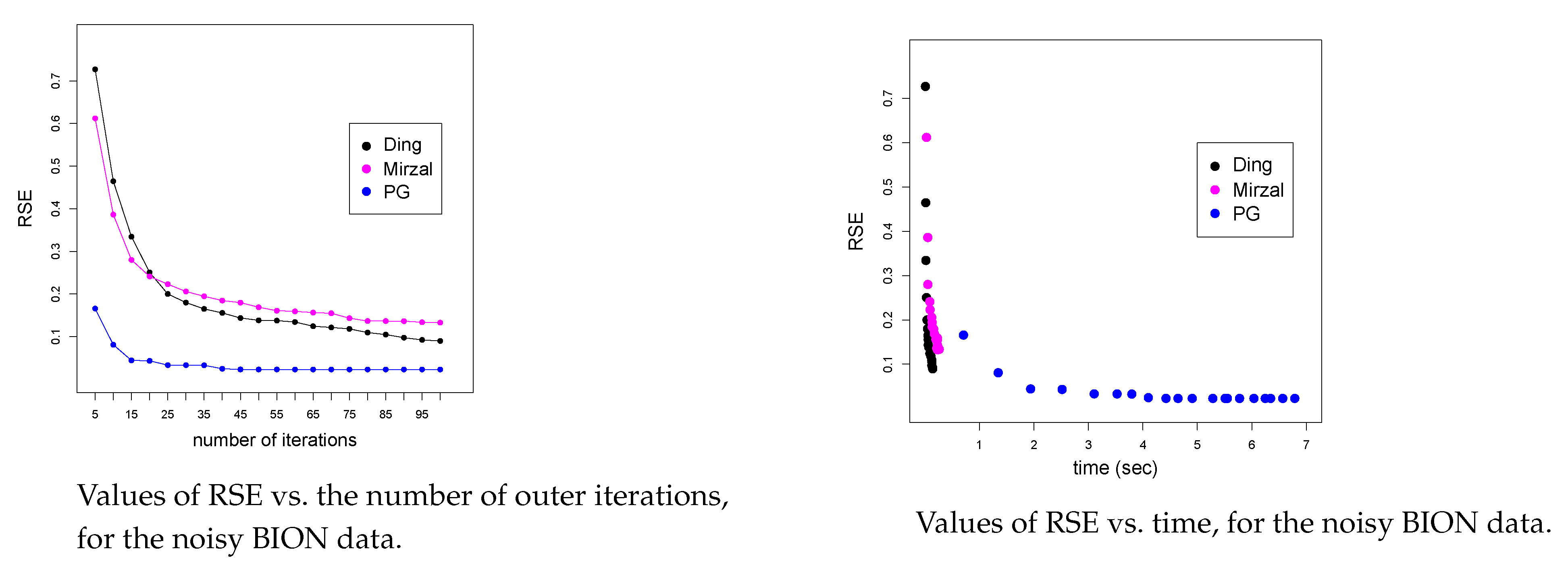
We first demonstrate how RSE decreases with iterations. The left plot in Figure 6 depicts that Algorithm 3 has the fastest decrease with the number of iterations and needs only a few dozens of iterations to reach optimum RSE. The other two algorithms need much more iterations. However, in each iteration, Algorithm 3 involves solving two sub-problems (9). This results in much higher times needed for one iteration. The right plot of Figure 6 depicts how RSE is decreasing with time. We can see that Algorithms 1 and 2 are much faster. We could decrease this difference by involving more advanced stopping criteria for Algorithm 3, which will be addressed during our future research.
5. Discussion and Conclusions
We presented a projected gradient method to solve the orthogonal non-negative matrix factorization problem. We penalized the deviation from orthonormality with some positive parameters and added the resulted terms to the objective function of the standard non-negative matrix factorization problem. Then, we considered minimizing the resulted objective function under the non-negativity conditions only, in a block coordinate decent approach. The method was tested on three sets of synthetic data: the first containing the uni-orthonormal matrices, the second containing the bi-orthonormal matrices and the third containing the noisy variants of the bi-orthonormal matrices. Different values for penalising parameters were applied in the implementation to determine recommendations which values shall be used in practise.
The performance of our algorithm was compared with two algorithms based on multiplicative updates rules. Algorithms were compared regarding the quality of factorization (RSE) and how much the resulting factors deviate from orthonormality. We provided an extensive list of numerical results which demonstrate that our method is very competitive and outperforms the others in terms of quality of the solution, measured by RSE, and feasibility of the solution, measured by or . If we take into account also the computing time, the Ding’s Algorithm 1 is also very competitive, since it computes solutions with slightly worse RSE and , but in much shorter time.
We expect that the difference in time complexity between Algorithms 1 and 3 can be reduced if we implement more advanced stopping criteria for the latter algorithm. This will be addressed in our future research.
Author Contributions
Methodology, S.A.; resources, J.P.; software, S.A. and J.P.; supervision, J.P. All authors have read and agreed to the published version of the manuscript.
Funding
The work of the first author is supported by the Swiss Government Excellence Scholarships grant number ESKAS-2019.0147. The work of the second author was partially funded by Slovenian Research Agency under research program P2-0162 and research projects J1-2453, N1-0071, J5-2552, J2-2512 and J1-1691.
Institutional Review Board Statement
Not applicable.
Informed Consent Statement
Not applicable.
Data Availability Statement
Data is available on git portal: https://github.com/Soodi1/ONMFdata (accessed on 8 November 2020).
Acknowledgments
The work of the first author is supported by the Swiss Government Excellence Scholarships grant number ESKAS-2019.0147. This author also thanks the University of Applied Sciences and Arts, Northwestern Switzerland for supporting the work. The work of the second author was partially funded by Slovenian Research Agency under research program P2-0162 and research projects J1-2453, N1-0071, J5-2552, J2-2512 and J1-1691. The authors would also like to thank to Andri Mirzal (Faculty of Computing, Universiti Teknologi Malaysia) for providing the code for his algorithm (Algorithm 2) to solve (ONMF). This code was also adapted by the authors to solve (bi-ONMF).
Conflicts of Interest
The authors declare no conflict of interest.
References
- Berry, M.W.; Browne, M.; Langville, A.N.; Pauca, V.P.; Plemmons, R.J. Algorithms and applications for approximate nonnegative matrix factorization. Comput. Stat. Data Anal. 2007, 52, 155–173. [Google Scholar] [CrossRef] [Green Version]
- Pauca, V.P.; Shahnaz, F.; Berry, M.W.; Plemmons, R.J. Text mining using non-negative matrix factorizations. In Proceedings of the 2004 SIAM International Conference on Data Mining, Lake Buena Vista, FL, USA, 22–24 April 2004; pp. 452–456. [Google Scholar]
- Shahnaz, F.; Berry, M.W.; Pauca, V.P.; Plemmons, R.J. Document clustering using nonnegative matrix factorization. Inf. Process. Manag. 2006, 42, 373–386. [Google Scholar] [CrossRef]
- Berry, M.W.; Gillis, N.; Glineur, F. Document classification using nonnegative matrix factorization and underapproximation. In Proceedings of the 2009 IEEE International Symposium on Circuits and Systems, Taipei, Taiwan, 24–27 May 2009; pp. 2782–2785. [Google Scholar]
- Li, T.; Ding, C. The relationships among various nonnegative matrix factorization methods for clustering. In Proceedings of the IEEE Sixth International Conference on Data Mining (ICDM’06), Hong Kong, China, 18–22 December 2006; pp. 362–371. [Google Scholar]
- Xu, W.; Liu, X.; Gong, Y. Document clustering based on non-negative matrix factorization. In Proceedings of the 26th Annual International ACM SIGIR Conference on Research and Development in Informaion Retrieval, Toronto, ON, Canada, 28 July–1 August 2003; pp. 267–273. [Google Scholar]
- Kaarna, A. Non-negative matrix factorization features from spectral signatures of AVIRIS images. In Proceedings of the 2006 IEEE International Symposium on Geoscience and Remote Sensing, Denver, CO, USA, 31 July–4 August 2006; pp. 549–552. [Google Scholar]
- Zafeiriou, S.; Tefas, A.; Buciu, I.; Pitas, I. Exploiting discriminant information in nonnegative matrix factorization with application to frontal face verification. IEEE Trans. Neural Netw. 2006, 17, 683–695. [Google Scholar] [CrossRef] [Green Version]
- Golub, G.H.; Reinsch, C. Singular value decomposition and least squares solutions. In Linear Algebra; Springer: Berlin, Germany, 1971; pp. 134–151. [Google Scholar]
- Jolliffe, I. Principal Component Analysis; Wiley Online Library: Hoboken, NJ, USA, 2005. [Google Scholar]
- Ding, C.; Li, T.; Peng, W.; Park, H. Orthogonal nonnegative matrix t-factorizations for clustering. In Proceedings of the 12th ACM SIGKDD International Conference on Knowledge Discovery and Data Mining, Philadelphia, PA, USA, 20–23 August 2006; pp. 126–135. [Google Scholar]
- Gillis, N. Nonnegative Matrix Factorization; Society for Industrial and Applied Mathematics: Philadelphia, PA, USA, 2020. [Google Scholar]
- Paatero, P.; Tapper, U. Positive matrix factorization: A non-negative factor model with optimal utilization of error estimates of data values. Environmetrics 1994, 5, 111–126. [Google Scholar] [CrossRef]
- Anttila, P.; Paatero, P.; Tapper, U.; Järvinen, O. Source identification of bulk wet deposition in Finland by positive matrix factorization. Atmos. Environ. 1995, 29, 1705–1718. [Google Scholar] [CrossRef]
- Lee, D.D.; Seung, H.S. Learning the parts of objects by non-negative matrix factorization. Nature 1999, 401, 788. [Google Scholar] [CrossRef] [PubMed]
- Lee, D.D.; Seung, H.S. Algorithms for non-negative matrix factorization. In Proceedings of the Advances in Neural Information Processing Systems, Denver, CO, USA, 27 November–2 December 2000; pp. 556–562. [Google Scholar]
- Chu, M.; Diele, F.; Plemmons, R.; Ragni, S. Optimality, computation, and interpretation of nonnegative matrix factorizations. SIAM J. Matrix Anal. 2004, 4, 8030. [Google Scholar]
- Kim, H.; Park, H. Nonnegative matrix factorization based on alternating nonnegativity constrained least squares and active set method. SIAM J. Matrix Anal. Appl. 2008, 30, 713–730. [Google Scholar] [CrossRef]
- Lin, C. Projected gradient methods for nonnegative matrix factorization. Neural Comput. 2007, 19, 2756–2779. [Google Scholar] [CrossRef] [PubMed] [Green Version]
- Cichocki, A.; Zdunek, R.; Amari, S.i. Hierarchical ALS algorithms for nonnegative matrix and 3D tensor factorization. In International Conference on Independent Component Analysis and Signal Separation; Springer: Berlin, Germany, 2007; pp. 169–176. [Google Scholar]
- Halko, N.; Martinsson, P.G.; Tropp, J.A. Finding structure with randomness: Probabilistic algorithms for constructing approximate matrix decompositions. SIAM Rev. 2011, 53, 217–288. [Google Scholar] [CrossRef]
- Yoo, J.; Choi, S. Orthogonal nonnegative matrix factorization: Multiplicative updates on Stiefel manifolds. In International Conference on Intelligent Data Engineering and Automated Learning; Springer: Berlin, Germany, 2008; pp. 140–147. [Google Scholar]
- Yoo, J.; Choi, S. Orthogonal nonnegative matrix tri-factorization for co-clustering: Multiplicative updates on stiefel manifolds. Inf. Process. Manag. 2010, 46, 559–570. [Google Scholar] [CrossRef]
- Choi, S. Algorithms for orthogonal nonnegative matrix factorization. In Proceedings of the 2008 IEEE International Joint Conference on Neural Networks (IEEE World Congress on Computational Intelligence), Hong Kong, China, 1–8 June 2008; pp. 1828–1832. [Google Scholar]
- Kim, D.; Sra, S.; Dhillon, I.S. Fast Projection-Based Methods for the Least Squares Nonnegative Matrix Approximation Problem. Stat. Anal. Data Mining 2008, 1, 38–51. [Google Scholar] [CrossRef] [Green Version]
- Kim, D.; Sra, S.; Dhillon, I.S. Fast Newton-type methods for the least squares nonnegative matrix approximation problem. In Proceedings of the 2007 SIAM International Conference on Data Mining, Minneapolis, MN, USA, 26–28 April 2007; pp. 343–354. [Google Scholar]
- Kim, J.; Park, H. Toward faster nonnegative matrix factorization: A new algorithm and comparisons. In Proceedings of the 2008 Eighth IEEE International Conference on Data Mining, Pisa, Italy, 15–19 December 2008; pp. 353–362. [Google Scholar]
- Mirzal, A. A convergent algorithm for orthogonal nonnegative matrix factorization. J. Comput. Appl. Math. 2014, 260, 149–166. [Google Scholar] [CrossRef]
- Lin, C.J. On the convergence of multiplicative update algorithms for nonnegative matrix factorization. IEEE Trans. Neural Netw. 2007, 18, 1589–1596. [Google Scholar]
- Esposito, F.; Boccarelli, A.; Del Buono, N. An NMF-Based methodology for selecting biomarkers in the landscape of genes of heterogeneous cancer-associated fibroblast Populations. Bioinform. Biol. Insights 2020, 14, 1–13. [Google Scholar] [CrossRef] [PubMed]
- Peng, S.; Ser, W.; Chen, B.; Lin, Z. Robust orthogonal nonnegative matrix tri-factorization for data representation. Knowl.-Based Syst. 2020, 201, 106054. [Google Scholar] [CrossRef]
- Leplat, N.V.; Gillis, A.A. Blind audio source separation with minimum-volume beta-divergence NMF. IEEE Trans. Signal Process. 2020, 68, 3400–3410. [Google Scholar] [CrossRef]
- Casalino, G.; Coluccia, M.; Pati, M.L.; Pannunzio, A.; Vacca, A.; Scilimati, A.; Perrone, M.G. Intelligent microarray data analysis through non-negative matrix factorization to study human multiple myeloma cell lines. Appl. Sci. 2019, 9, 5552. [Google Scholar] [CrossRef] [Green Version]
- Ge, S.; Luo, L.; Li, H. Orthogonal incremental non-negative matrix factorization algorithm and its application in image classification. Comput. Appl. Math. 2020, 39, 1–16. [Google Scholar] [CrossRef]
- Bertsekas, D. Nonlinear Programming; Athena Scientific optimization and Computation Series; Athena Scientific: Nashua, NH, USA, 2016. [Google Scholar]
- Richtárik, P.; Takác, M. Iteration complexity of randomized block-coordinate descent methods for minimizing a composite function. Math. Program. 2014, 144, 1–38. [Google Scholar] [CrossRef] [Green Version]
- The MathWorks. MATLAB Version R2019a; The MathWorks: Natick, MA, USA, 2019. [Google Scholar]
- Cichocki, A.; Zdunek, R.; Phan, A.H.; Amari, S.i. Nonnegative Matrix and Tensor Factorizations: Applications to Exploratory Multi-Way Data Analysis and Blind Source Separation; John Wiley & Sons: Hoboken, NJ, USA, 2009. [Google Scholar]
- Piper, J.; Pauca, V.P.; Plemmons, R.J.; Giffin, M. Object Characterization from Spectral Data Using Nonnegative Factorization and Information theory. In Proceedings of the AMOS Technical Conference; 2004. Available online: http://users.wfu.edu/plemmons/papers/Amos2004_2.pdf (accessed on 8 November 2020).
- Mirzal, A. A Convergent Algorithm for Bi-orthogonal Nonnegative Matrix Tri-Factorization. arXiv 2017, arXiv:1710.11478. [Google Scholar]
- Armijo, L. Minimization of functions having Lipschitz continuous first partial derivatives. Pac. J. Math. 1966, 16, 1–3. [Google Scholar] [CrossRef] [Green Version]
- Lin, C.J.; Moré, J.J. Newton’s method for large bound-constrained optimization problems. SIAM J. Optim. 1999, 9, 1100–1127. [Google Scholar] [CrossRef] [Green Version]
Figure 1.
This figure depicts data from Table 2. It contains six plots which illustrate the quality of Algorithms 1–3 regarding RSE on UNION instances with n = 100, 500, 1000, for β ∊ {1, 10, 100, 1000}. We can see that regarding RSE the performance of these algorithms on this dataset does not differ a lot. As expected, larger values of β yield larger values of RSE, but the differences are rather small. However, when p approached 100% of k, Algorithm 3 comes closest to the global optimum RSE = 0.

Figure 2.
This figure depicts data from Table 3. It contains six plots which illustrate the quality of Algorithms 1–3 regarding infeasibility on UNION instances with n = 100, 500, 1000, for β ∊ {1, 10, 100, 1000}. We can see that regarding infeasibility the performance of these algorithms on this dataset does not differ a lot. As expected, larger values of β yield smaller values of infeasG, but the differences are rather small.

Figure 3.
This figure contains six plots which illustrate the quality of Algorithms 1–3 regarding RSE on BION instances with n = 100, 500, 1000 and k = 0.2n, 0.4n, for β ∊ {1, 10, 100, 1000}. We can observe that Algorithm 3 is more stable, less dependent to the choice of β and is computing better values of RSE.

Figure 4.
This figure contains six plots which illustrate the quality of Algorithms 1–3 regarding the infeasibility on BION instances with n = 100, 500, 1000 and k = 0.2n, 0.4n, for β ∊ {1, 10, 100, 1000}. We can observe that Algorithm 3 computes solutions with infeasibility (18) slightly smaller compared to solutions computed by Algorithm 2.

Figure 5.
On the left, we depict how RSE is changing with increasing the inner dimension p from 20% of real inner dimension k to 140% of k. For each algorithm, we depict RSE on the original BION data and on the noisy BION data with µ ∊ {10−2, 10−4, 10−6}. On the right plots, we demonstrate how (in)feasible are the optimum solutions obtained by each algorithm, for different relative inner dimensions p, for the original and the noisy BION data.

Figure 6.
This figure depicts how RSE is changing with the number of outer iterations (left) and with time (right), for all three algorithms. Computations are done on the noisy BION data set with µ = 10−2, for n = 200 and the inner dimension was equal to the true inner dimension (p = 100 %).
Figure 6.
This figure depicts how RSE is changing with the number of outer iterations (left) and with time (right), for all three algorithms. Computations are done on the noisy BION data set with µ = 10−2, for n = 200 and the inner dimension was equal to the true inner dimension (p = 100 %).


Table 1.
Paris for which we created UNION and BION datasets.
| n | 50 | 100 | 200 | 500 | 1000 |
|---|---|---|---|---|---|
| k | 10 | 20 | 40 | 100 | 200 |
| k | 20 | 40 | 80 | 200 | 400 |
Table 2.
In this table we demonstrate how good RSE is achieved by Algorithms 1–3 on UNION dataset. For each we take all 10 matrices R (five of them corresponding to and five to ). We run all three algorithms on these matrices with inner dimensions with all possible values of . Each row represents the average (arithmetic mean value) RSE obtained on instances corresponding to given n. For example, the last row shows the average value of RSE in 10 instances of dimension 1000 (five of them corresponding to and five to ) obtained by all three algorithms for all four values of , which were run with the input dimension . The bold number is the smallest one in each line.
| n | p | RSE of | RSE of Algorithm 2 | RSE of Algorithm 3 | ||||||
|---|---|---|---|---|---|---|---|---|---|---|
| (% of k) | Algorithm 1 | |||||||||
| 50 | 40 | 0.3143 | 0.2965 | 0.3070 | 0.3329 | 0.3898 | 0.2963 | 0.3081 | 0.3425 | 0.3508 |
| 50 | 60 | 0.2348 | 0.2227 | 0.2356 | 0.2676 | 0.3459 | 0.2201 | 0.2382 | 0.2733 | 0.2765 |
| 50 | 80 | 0.1738 | 0.1492 | 0.1634 | 0.1894 | 0.3277 | 0.1468 | 0.1620 | 0.1953 | 0.2053 |
| 50 | 100 | 0.0002 | 0.0133 | 0.0004 | 0.0932 | 0.2973 | 0.0000 | 0.0000 | 0.0000 | 0.0000 |
| 100 | 20 | 0.4063 | 0.3914 | 0.3955 | 0.4063 | 0.4254 | 0.3906 | 0.3959 | 0.4083 | 0.4210 |
| 100 | 40 | 0.3384 | 0.3139 | 0.3210 | 0.3415 | 0.3677 | 0.3116 | 0.3210 | 0.3488 | 0.3625 |
| 100 | 60 | 0.2674 | 0.2462 | 0.2541 | 0.2730 | 0.2978 | 0.2403 | 0.2528 | 0.2801 | 0.2974 |
| 100 | 80 | 0.1847 | 0.1737 | 0.1581 | 0.1909 | 0.2263 | 0.1629 | 0.1744 | 0.1959 | 0.2090 |
| 100 | 100 | 0.0126 | 0.0532 | 0.0427 | 0.0089 | 0.1515 | 0.0000 | 0.0000 | 0.0000 | 0.0075 |
| 200 | 20 | 0.4213 | 0.4024 | 0.4077 | 0.4080 | 0.4257 | 0.4005 | 0.4032 | 0.4162 | 0.4337 |
| 200 | 40 | 0.3562 | 0.3315 | 0.3398 | 0.3401 | 0.3647 | 0.3270 | 0.3313 | 0.3497 | 0.3738 |
| 200 | 60 | 0.2845 | 0.2675 | 0.2746 | 0.2748 | 0.2955 | 0.2573 | 0.2617 | 0.2812 | 0.3061 |
| 200 | 80 | 0.1959 | 0.1958 | 0.2013 | 0.1996 | 0.2085 | 0.1773 | 0.1819 | 0.1960 | 0.2133 |
| 200 | 100 | 0.0191 | 0.0753 | 0.0632 | 0.0622 | 0.0415 | 0.0000 | 0.0000 | 0.0069 | 0.0181 |
| 500 | 20 | 0.4332 | 0.4120 | 0.4119 | 0.4120 | 0.4121 | 0.4092 | 0.4096 | 0.4197 | 0.4346 |
| 500 | 40 | 0.3711 | 0.3506 | 0.3509 | 0.3507 | 0.3505 | 0.3430 | 0.3440 | 0.3537 | 0.3753 |
| 500 | 60 | 0.3003 | 0.2919 | 0.2923 | 0.2916 | 0.2909 | 0.2756 | 0.2766 | 0.2845 | 0.3031 |
| 500 | 80 | 0.2098 | 0.2186 | 0.2192 | 0.2207 | 0.2151 | 0.1931 | 0.1941 | 0.1999 | 0.2122 |
| 500 | 100 | 0.0273 | 0.0822 | 0.0864 | 0.0853 | 0.0713 | 0.0002 | 0.0003 | 0.0002 | 0.0097 |
| 1000 | 20 | 0.4386 | 0.4195 | 0.4194 | 0.4193 | 0.4195 | 0.4156 | 0.4160 | 0.4216 | 0.4324 |
| 1000 | 40 | 0.3777 | 0.3641 | 0.3640 | 0.3638 | 0.3637 | 0.3545 | 0.3548 | 0.3588 | 0.3707 |
| 1000 | 60 | 0.3070 | 0.3047 | 0.3055 | 0.3051 | 0.3036 | 0.2881 | 0.2880 | 0.2906 | 0.3006 |
| 1000 | 80 | 0.2164 | 0.2265 | 0.2248 | 0.2254 | 0.2236 | 0.2024 | 0.2029 | 0.2050 | 0.2106 |
| 1000 | 100 | 0.0329 | 0.0725 | 0.0772 | 0.0761 | 0.0709 | 0.0173 | 0.0030 | 0.0035 | 0.0035 |
Table 3.
In this table we demonstrate how feasible (orthonormal) the solutions are G computed by Algorithms 1–3 on UNION data set, i.e., in this table we report the average infeasibility of the solutions underlying Table 2. The bold number is the smallest one in each line.
Table 3.
In this table we demonstrate how feasible (orthonormal) the solutions are G computed by Algorithms 1–3 on UNION data set, i.e., in this table we report the average infeasibility of the solutions underlying Table 2. The bold number is the smallest one in each line.
| n | p | Infeas. of | Infeas. of Algorithm 2 | Infeas. of Algorithm 3 | ||||||
|---|---|---|---|---|---|---|---|---|---|---|
| (% of k) | Algorithm 1 | |||||||||
| 50 | 20 | 0.0964 | 0.2490 | 0.0924 | 0.0155 | 0.0038 | 0.2298 | 0.0909 | 0.0154 | 0.0022 |
| 50 | 40 | 0.0740 | 0.1886 | 0.0676 | 0.0131 | 0.0040 | 0.1845 | 0.0670 | 0.0135 | 0.0023 |
| 50 | 60 | 0.0553 | 0.1324 | 0.0465 | 0.0068 | 0.0040 | 0.1245 | 0.0440 | 0.0091 | 0.0015 |
| 50 | 80 | 0.0324 | 0.0964 | 0.0241 | 0.0053 | 0.0034 | 0.0789 | 0.0250 | 0.0069 | 0.0020 |
| 50 | 100 | 0.0023 | 0.0257 | 0.0022 | 0.0023 | 0.0039 | 0.0000 | 0.0000 | 0.0000 | 0.0000 |
| 100 | 20 | 0.0774 | 0.2624 | 0.1441 | 0.0258 | 0.0064 | 0.2588 | 0.1308 | 0.0258 | 0.0036 |
| 100 | 40 | 0.0539 | 0.1754 | 0.0928 | 0.0168 | 0.0036 | 0.1654 | 0.0819 | 0.0182 | 0.0035 |
| 100 | 60 | 0.0400 | 0.1205 | 0.0545 | 0.0102 | 0.0024 | 0.1109 | 0.0487 | 0.0138 | 0.0033 |
| 100 | 80 | 0.0239 | 0.0890 | 0.0324 | 0.0062 | 0.0022 | 0.0623 | 0.0258 | 0.0083 | 0.0018 |
| 100 | 100 | 0.0062 | 0.0452 | 0.0153 | 0.0009 | 0.0016 | 0.0002 | 0.0000 | 0.0000 | 0.0000 |
| 200 | 20 | 0.0584 | 0.2157 | 0.1437 | 0.1433 | 0.0054 | 0.2087 | 0.1512 | 0.0348 | 0.0074 |
| 200 | 40 | 0.0356 | 0.1379 | 0.1004 | 0.1000 | 0.0036 | 0.1240 | 0.0806 | 0.0207 | 0.0053 |
| 200 | 60 | 0.0260 | 0.0955 | 0.0791 | 0.0793 | 0.0031 | 0.0754 | 0.0434 | 0.0143 | 0.0047 |
| 200 | 80 | 0.0154 | 0.0657 | 0.0634 | 0.0629 | 0.0017 | 0.0416 | 0.0218 | 0.0080 | 0.0026 |
| 200 | 100 | 0.0059 | 0.0412 | 0.0517 | 0.0512 | 0.0016 | 0.0002 | 0.0001 | 0.0002 | 0.0001 |
| 500 | 20 | 0.0332 | 0.1587 | 0.1894 | 0.1908 | 0.1908 | 0.1475 | 0.1268 | 0.0436 | 0.0087 |
| 500 | 40 | 0.0189 | 0.1155 | 0.1343 | 0.1349 | 0.1347 | 0.0770 | 0.0621 | 0.0227 | 0.0069 |
| 500 | 60 | 0.0134 | 0.0889 | 0.1095 | 0.1102 | 0.1055 | 0.0412 | 0.0312 | 0.0123 | 0.0038 |
| 500 | 80 | 0.0084 | 0.0656 | 0.0946 | 0.0954 | 0.0826 | 0.0300 | 0.0154 | 0.0061 | 0.0021 |
| 500 | 100 | 0.0050 | 0.0499 | 0.0847 | 0.0853 | 0.0693 | 0.0249 | 0.0003 | 0.0001 | 0.0001 |
| 1000 | 20 | 0.0211 | 0.1200 | 0.1344 | 0.1349 | 0.1350 | 0.1043 | 0.0970 | 0.0471 | 0.0097 |
| 1000 | 40 | 0.0122 | 0.0863 | 0.0951 | 0.0954 | 0.0954 | 0.0542 | 0.0422 | 0.0199 | 0.0059 |
| 1000 | 60 | 0.0073 | 0.0662 | 0.0776 | 0.0779 | 0.0779 | 0.0414 | 0.0205 | 0.0098 | 0.0037 |
| 1000 | 80 | 0.0045 | 0.0539 | 0.0671 | 0.0675 | 0.0675 | 0.0336 | 0.0103 | 0.0047 | 0.0018 |
| 1000 | 100 | 0.0040 | 0.0475 | 0.0600 | 0.0603 | 0.0604 | 0.0296 | 0.0066 | 0.0005 | 0.0003 |
Table 4.
RSE obtained by Algorithms 1–3 on the BION data. For the latter two algorithms, we used . For each we take all ten matrices R (five of them corresponding to and five to ). We run all three algorithms on these matrices with inner dimensions with all possible values of . Like before, each row represents the average (arithmetic mean value) of RSE obtained on instances corresponding to given n and given p as a percentage of k. We can see that the larger the , the worse the RSE, which is consistent with expectations. The bold number is the smallest one in each line.
| n | p | RSE of | RSE of Algorithm 2 | RSE of Algorithm 3 | ||||||
|---|---|---|---|---|---|---|---|---|---|---|
| (% of k) | Algorithm 1 | |||||||||
| 50 | 20 | 0.7053 | 0.7053 | 0.7053 | 0.7053 | 0.8283 | 0.7053 | 0.7053 | 0.7055 | 0.8259 |
| 50 | 40 | 0.6108 | 0.6108 | 0.6108 | 0.6108 | 0.9066 | 0.6108 | 0.6108 | 0.6108 | 0.6631 |
| 50 | 60 | 0.4987 | 0.4987 | 0.4987 | 0.5442 | 0.9665 | 0.4987 | 0.4987 | 0.4987 | 0.5000 |
| 50 | 80 | 0.3526 | 0.3671 | 0.3742 | 0.4497 | 1.0282 | 0.3526 | 0.3796 | 0.3527 | 0.4374 |
| 50 | 100 | 0.0607 | 0.1712 | 0.2786 | 0.5198 | 1.0781 | 0.1145 | 0.1820 | 0.2604 | 0.3689 |
| 100 | 20 | 0.7516 | 0.7516 | 0.7516 | 0.7517 | 0.9070 | 0.7516 | 0.7516 | 0.7517 | 0.8224 |
| 100 | 40 | 0.6509 | 0.6509 | 0.6509 | 0.7174 | 0.9779 | 0.6509 | 0.6509 | 0.6509 | 0.6514 |
| 100 | 60 | 0.5315 | 0.5315 | 0.5315 | 0.5504 | 1.0401 | 0.5315 | 0.5315 | 0.5315 | 0.5352 |
| 100 | 80 | 0.3758 | 0.3787 | 0.4106 | 0.4542 | 1.1082 | 0.3801 | 0.3888 | 0.3917 | 0.3898 |
| 100 | 100 | 0.1377 | 0.1993 | 0.3311 | 0.4898 | 1.1734 | 0.0457 | 0.1016 | 0.2758 | 0.3757 |
| 200 | 20 | 0.7884 | 0.7884 | 0.7884 | 0.7884 | 0.9499 | 0.7884 | 0.7884 | 0.7884 | 0.7888 |
| 200 | 40 | 0.6828 | 0.6828 | 0.6828 | 0.6828 | 1.0325 | 0.6828 | 0.6828 | 0.6828 | 0.6828 |
| 200 | 60 | 0.5575 | 0.5575 | 0.5575 | 0.5647 | 1.0938 | 0.5575 | 0.5575 | 0.5575 | 0.5610 |
| 200 | 80 | 0.3942 | 0.3942 | 0.3965 | 0.5019 | 1.1618 | 0.3942 | 0.3942 | 0.3942 | 0.4373 |
| 200 | 100 | 0.1447 | 0.1851 | 0.3014 | 0.5400 | 1.2297 | 0.0202 | 0.1429 | 0.2964 | 0.3315 |
| 500 | 20 | 0.8242 | 0.8242 | 0.8242 | 0.8242 | 0.9956 | 0.8242 | 0.8242 | 0.8242 | 0.8243 |
| 500 | 40 | 0.7138 | 0.7138 | 0.7138 | 0.7138 | 1.0679 | 0.7138 | 0.7138 | 0.7138 | 0.7138 |
| 500 | 60 | 0.5828 | 0.5828 | 0.5828 | 0.6045 | 1.1534 | 0.5828 | 0.5828 | 0.5828 | 0.5828 |
| 500 | 80 | 0.4121 | 0.4121 | 0.4203 | 0.5285 | 1.2160 | 0.4121 | 0.4121 | 0.4121 | 0.4334 |
| 500 | 100 | 0.1405 | 0.1814 | 0.3401 | 0.5854 | 1.2822 | 0.0067 | 0.1059 | 0.2044 | 0.3378 |
| 1000 | 20 | 0.8436 | 0.8436 | 0.8436 | 0.8436 | 1.0261 | 0.8436 | 0.8436 | 0.8436 | 0.8436 |
| 1000 | 40 | 0.7306 | 0.7306 | 0.7306 | 0.7309 | 1.0916 | 0.7306 | 0.7306 | 0.7306 | 0.7306 |
| 1000 | 60 | 0.5965 | 0.5965 | 0.5965 | 0.6121 | 1.1669 | 0.5965 | 0.5965 | 0.5965 | 0.5968 |
| 1000 | 80 | 0.4218 | 0.4218 | 0.4256 | 0.5338 | 1.2389 | 0.4218 | 0.4218 | 0.4218 | 0.4397 |
| 1000 | 100 | 0.1346 | 0.1635 | 0.3324 | 0.5755 | 1.3080 | 0.0096 | 0.0697 | 0.1661 | 0.2188 |
Table 5.
In this table we demonstrate how feasible (orthonormal) are the solutions G and H computed by Algorithms 1–3 on the BION dataset, i.e., in this table we report the average infeasibility (18) of the solutions underlying Table 4. We can observe that with these settings of all algorithms we can bring infeasibility to order of very often, for all values of . The bold number is the smallest one in each line.
| n | p | Infeas. of | Infeas. of Algorithm 2 | Infeas. of Algorithm 3 | ||||||
|---|---|---|---|---|---|---|---|---|---|---|
| (% of k) | Algorithm 1 | |||||||||
| 50 | 20 | 0.0001 | 0.0070 | 0.0036 | 0.0010 | 0.0068 | 0.0017 | 0.0021 | 0.0021 | 0.0026 |
| 50 | 40 | 0.0000 | 0.0041 | 0.0021 | 0.0004 | 0.0056 | 0.0008 | 0.0012 | 0.0012 | 0.0014 |
| 50 | 60 | 0.0000 | 0.0030 | 0.0009 | 0.0032 | 0.0038 | 0.0005 | 0.0008 | 0.0009 | 0.0009 |
| 50 | 80 | 0.0000 | 0.0183 | 0.0030 | 0.0021 | 0.0028 | 0.0004 | 0.0202 | 0.0006 | 0.0013 |
| 50 | 100 | 0.0355 | 0.0533 | 0.0127 | 0.0045 | 0.0027 | 0.0418 | 0.0478 | 0.0123 | 0.0021 |
| 100 | 20 | 0.0001 | 0.0051 | 0.0024 | 0.0006 | 0.0063 | 0.0010 | 0.0012 | 0.0013 | 0.0016 |
| 100 | 40 | 0.0000 | 0.0029 | 0.0017 | 0.0066 | 0.0040 | 0.0004 | 0.0006 | 0.0007 | 0.0007 |
| 100 | 60 | 0.0000 | 0.0019 | 0.0008 | 0.0009 | 0.0027 | 0.0003 | 0.0004 | 0.0005 | 0.0005 |
| 100 | 80 | 0.0000 | 0.0039 | 0.0048 | 0.0015 | 0.0021 | 0.0062 | 0.0149 | 0.0037 | 0.0006 |
| 100 | 100 | 0.0606 | 0.0454 | 0.0105 | 0.0022 | 0.0018 | 0.0106 | 0.0228 | 0.0173 | 0.0028 |
| 200 | 20 | 0.0002 | 0.0033 | 0.0019 | 0.0005 | 0.0043 | 0.0005 | 0.0007 | 0.0007 | 0.0007 |
| 200 | 40 | 0.0001 | 0.0017 | 0.0010 | 0.0002 | 0.0027 | 0.0002 | 0.0003 | 0.0004 | 0.0003 |
| 200 | 60 | 0.0001 | 0.0010 | 0.0005 | 0.0004 | 0.0019 | 0.0001 | 0.0002 | 0.0002 | 0.0004 |
| 200 | 80 | 0.0000 | 0.0006 | 0.0006 | 0.0015 | 0.0014 | 0.0001 | 0.0001 | 0.0002 | 0.0013 |
| 200 | 100 | 0.0425 | 0.0280 | 0.0064 | 0.0019 | 0.0015 | 0.0046 | 0.0224 | 0.0240 | 0.0034 |
| 500 | 20 | 0.0001 | 0.0017 | 0.0011 | 0.0003 | 0.0025 | 0.0002 | 0.0003 | 0.0003 | 0.0003 |
| 500 | 40 | 0.0001 | 0.0008 | 0.0005 | 0.0001 | 0.0016 | 0.0001 | 0.0001 | 0.0002 | 0.0002 |
| 500 | 60 | 0.0000 | 0.0005 | 0.0003 | 0.0006 | 0.0013 | 0.0001 | 0.0001 | 0.0001 | 0.0002 |
| 500 | 80 | 0.0000 | 0.0003 | 0.0009 | 0.0009 | 0.0008 | 0.0000 | 0.0001 | 0.0001 | 0.0016 |
| 500 | 100 | 0.0258 | 0.0184 | 0.0045 | 0.0013 | 0.0007 | 0.0017 | 0.0101 | 0.0175 | 0.0053 |
| 1000 | 20 | 0.0001 | 0.0010 | 0.0006 | 0.0002 | 0.0024 | 0.0001 | 0.0002 | 0.0002 | 0.0002 |
| 1000 | 40 | 0.0000 | 0.0005 | 0.0003 | 0.0001 | 0.0009 | 0.0001 | 0.0002 | 0.0003 | 0.0002 |
| 1000 | 60 | 0.0000 | 0.0003 | 0.0002 | 0.0004 | 0.0009 | 0.0003 | 0.0002 | 0.0003 | 0.0003 |
| 1000 | 80 | 0.0000 | 0.0002 | 0.0005 | 0.0007 | 0.0006 | 0.0040 | 0.0001 | 0.0002 | 0.0020 |
| 1000 | 100 | 0.0173 | 0.0117 | 0.0031 | 0.0009 | 0.0005 | 0.0043 | 0.0050 | 0.0121 | 0.0060 |
Table 6.
This table contains numerical data obtained by running all three algorithms on the third dataset—BION data with three levels of noise, represented by . The bold number is the smallest one in each line.
Table 6.
This table contains numerical data obtained by running all three algorithms on the third dataset—BION data with three levels of noise, represented by . The bold number is the smallest one in each line.
| Algorithm 1 | Algorithm 2 | Algorithm 3 | |||||||||
|---|---|---|---|---|---|---|---|---|---|---|---|
| RSE | RSE | RSE | |||||||||
| 20 | 200 | 0.7877 | 0.0019 | 0.0019 | 0.7877 | 0.0041 | 0.0041 | 0.7877 | 0.0042 | 0.0042 | |
| 40 | 200 | 0.6821 | 0.0014 | 0.0014 | 0.6823 | 0.0024 | 0.0024 | 0.6821 | 0.0027 | 0.0028 | |
| 60 | 200 | 0.5570 | 0.0010 | 0.0010 | 0.5571 | 0.0015 | 0.0015 | 0.5569 | 0.0020 | 0.0020 | |
| 80 | 200 | 0.3939 | 0.0007 | 0.0007 | 0.3939 | 0.0010 | 0.0010 | 0.3938 | 0.0015 | 0.0015 | |
| 100 | 200 | 0.0072 | 0.0003 | 0.0003 | 0.1327 | 0.0097 | 0.0098 | 0.0039 | 0.0010 | 0.0010 | |
| 120 | 200 | 0.0278 | 0.0483 | 0.0483 | 0.1325 | 0.0283 | 0.0326 | 0.0036 | 0.0465 | 0.0141 | |
| 140 | 200 | 0.0344 | 0.0589 | 0.0590 | 0.1909 | 0.0366 | 0.0363 | 0.0034 | 0.0565 | 0.0188 | |
| 20 | 200 | 0.7884 | 0.0002 | 0.0002 | 0.7884 | 0.0018 | 0.0018 | 0.7884 | 0.0003 | 0.0003 | |
| 40 | 200 | 0.6828 | 0.0001 | 0.0001 | 0.6828 | 0.0009 | 0.0009 | 0.6828 | 0.0001 | 0.0001 | |
| 60 | 200 | 0.5575 | 0.0001 | 0.0001 | 0.5575 | 0.0006 | 0.0006 | 0.5575 | 0.0001 | 0.0001 | |
| 80 | 200 | 0.3942 | 0.0000 | 0.0000 | 0.3942 | 0.0004 | 0.0003 | 0.3942 | 0.0001 | 0.0001 | |
| 100 | 200 | 0.0575 | 0.0086 | 0.0086 | 0.1717 | 0.0089 | 0.0192 | 0.0001 | 0.0004 | 0.0004 | |
| 120 | 200 | 0.0043 | 0.0490 | 0.0489 | 0.1407 | 0.0275 | 0.0321 | 0.0003 | 0.0468 | 0.0159 | |
| 140 | 200 | 0.0049 | 0.0596 | 0.0596 | 0.1743 | 0.0363 | 0.0390 | 0.0003 | 0.0558 | 0.0221 | |
| 20 | 200 | 0.7884 | 0.0001 | 0.0001 | 0.7884 | 0.0017 | 0.0017 | 0.7884 | 0.0002 | 0.0002 | |
| 40 | 200 | 0.6828 | 0.0000 | 0.0000 | 0.6828 | 0.0009 | 0.0008 | 0.6828 | 0.0001 | 0.0001 | |
| 60 | 200 | 0.5575 | 0.0000 | 0.0000 | 0.5575 | 0.0005 | 0.0005 | 0.5575 | 0.0001 | 0.0001 | |
| 80 | 200 | 0.3942 | 0.0000 | 0.0000 | 0.3942 | 0.0003 | 0.0003 | 0.3942 | 0.0001 | 0.0001 | |
| 100 | 200 | 0.0624 | 0.0092 | 0.0091 | 0.1966 | 0.0159 | 0.0167 | 0.0137 | 0.0029 | 0.0006 | |
| 120 | 200 | 0.0031 | 0.0490 | 0.0492 | 0.1250 | 0.0301 | 0.0309 | 0.0003 | 0.0478 | 0.0179 | |
| 140 | 200 | 0.0051 | 0.0595 | 0.0597 | 0.1692 | 0.0367 | 0.0381 | 0.0003 | 0.0562 | 0.0268 | |
Publisher’s Note: MDPI stays neutral with regard to jurisdictional claims in published maps and institutional affiliations. |
© 2021 by the authors. Licensee MDPI, Basel, Switzerland. This article is an open access article distributed under the terms and conditions of the Creative Commons Attribution (CC BY) license (http://creativecommons.org/licenses/by/4.0/).
Share and Cite
MDPI and ACS Style
Asadi, S.; Povh, J. A Block Coordinate Descent-Based Projected Gradient Algorithm for Orthogonal Non-Negative Matrix Factorization. Mathematics 2021, 9, 540. https://doi.org/10.3390/math9050540
AMA Style
Asadi S, Povh J. A Block Coordinate Descent-Based Projected Gradient Algorithm for Orthogonal Non-Negative Matrix Factorization. Mathematics. 2021; 9(5):540. https://doi.org/10.3390/math9050540
Chicago/Turabian StyleAsadi, Soodabeh, and Janez Povh. 2021. "A Block Coordinate Descent-Based Projected Gradient Algorithm for Orthogonal Non-Negative Matrix Factorization" Mathematics 9, no. 5: 540. https://doi.org/10.3390/math9050540
Note that from the first issue of 2016, this journal uses article numbers instead of page numbers. See further details here.