
Numerical Modeling of the Spread of Cough Saliva Droplets in a Calm Confined Space
by
 , , and
Sergio A. Chillón
1, 
Ainara Ugarte-Anero
1,
Iñigo Aramendia
1,
Unai Fernandez-Gamiz
1,* and
and
Ekaitz Zulueta
2 1
Nuclear Engineering and Fluid Mechanics Department, University of the Basque Country, UPV/EHU, Nieves Cano 12, Vitoria-Gasteiz, 01006 Araba, Spain
2
System Engineering and Automation Control Department, University of the Basque Country, UPV/EHU, Nieves Cano 12, Vitoria-Gasteiz, 01006 Araba, Spain
*
Author to whom correspondence should be addressed.
Mathematics 2021, 9(5), 574; https://doi.org/10.3390/math9050574
Submission received: 21 January 2021
/
Revised: 22 February 2021
/
Accepted: 1 March 2021
/
Published: 8 March 2021
(This article belongs to the Special Issue Mathematical and Computational Methods against the COVID-19 Pandemics)
Abstract
:The coronavirus disease 2019 (COVID-19) outbreak has altered the lives of everyone on a global scale due to its high transmission rate. In the current work, the droplet dispersion and evaporation originated by a cough at different velocities is studied. A multiphase computational fluid dynamic model based on fully coupled Eulerian–Lagrangian techniques was used. The evaporation, breakup, mass transfer, phase change, and turbulent dispersion forces of droplets were taken into account. A computational domain imitating an elevator that with two individuals inside was modeled. The results showed that all droplets smaller than 150 μm evaporate before 10 s at different heights. Smaller droplets of <30 µm evaporate quickly, and their trajectories are governed by Brownian movements. Instead, the trajectories of medium-sized droplets (30–80 µm) are under the influence of inertial forces, while bigger droplets move according to inertial and gravitational forces. Smaller droplets are located in the top positions, while larger (i.e., heaviest) droplets are located at the bottom.
1. Introduction
Coronavirus disease 2019 (COVID-19) is the third coronavirus of the 21st century. The first detected coronavirus was severe acute respiratory syndrome (SARS), which surged in 2002 in China and caused 8000 infections and 774 deaths. In 2012, the Middle East Respiratory Syndrome (MERS) appeared in Arabia Saudi, causing 2494 infections and 858 deaths. In December of 2019, COVID-19 virus was officially detected in Wuhan, China. This virus spread severely, potentially supported by the Chinese New Year. In March, more than 96,000 cases were reported in 87 countries. Currently, the spread of this coronavirus has caused more than 95.1 million infections and more than 2.03 million deaths worldwide. This virus has affected the public, the economy, and the global health. The initial control measures were isolation, increasing social distancing, and wearing masks [1]. Controlling this pandemic has been the priority challenge of the world, and thus, it is necessary to understand the main mechanisms of the transmission of the virus. The spread of this virus is greater by airborne means, especially in indoor environments, as stated by Moriyama et al. [2]. According to Vuorinen et al. [3] and Morawska et al. [4], inhaling small droplets is probably the third cause of infection of COVID-19, after inhaling larger droplets and by contact with infected people or surfaces. According to [4], the WHO (World Health Organization) has not recognized as strongly as needed the transmission in small closed places by inhaling small droplets, but some ventilation engineering organizations such as REHVA and ASHRAE has, recognizing the airborne risk in virus-laden indoor spaces and recommending to control ventilation. A favorable ventilation system can prevent high infection risks, whereas a badly designed ventilation system could be worse than a closed room [4]. Many hospitals are equipped with natural forced ventilation systems and the WHO has recommended a minimum ventilation of 160 L/s for safety in these installations. According to van Doremalen et al. [5], COVID-19 has an average lifetime of more than 1 h when airborne.
Aerosols can be defined as solid or liquid particles in the air. Those aerosols spread from being person-borne to airborne principally by breathing, talking, coughing, or sneezing. These droplets evaporate quickly but leave a residue that can be transported as a pathogen whose buoyancy can last for several minutes [3,6]. Consequently, the WHO has recommended a social distancing limit of 1.8 m (6 feet). Several studies have agreed that this distance is correct for large droplets when there is no airflow (Vair = 0), but that it is insufficient when the Vair is different to zero or when aerosol particles need to be prevented. In the case of a soft breeze (4 km/h), aerosols can travel for more than 6 m in only 5 s [6,7]. Other recommendations are to avoid the recirculation of air, to use devices to clean and disinfect the air, and, over all, to minimize the number of persons indoors [4]. Moreover, it is recommendable to use surgical masks to prevent the spread of particles. Dbouk et al. [8] showed that surgical masks trap most droplets, and although leaked droplets can travel several meters depending on the airborne conditions, the concentration will be lower, as will be the risk of infection. In addition to leaked droplets, another problematic issue is their dynamic efficiency (see Busco et al. [9]).
Several studies are available in the literature regarding the behavior of droplets. Asadi et al. [10] studied how droplets are expelled during speaking and measured the droplet rate using an aerodynamic particle sizer (APS) during different speeches. They concluded that vocal folds throw more droplets and that the emission rate increases with amplitude, but not with the size distribution. Busco et al. [9] applied the body movements to a computational fluid dynamics (CFD) mannequin during sneezing, concluding that these movements, in a realistic dynamic pressure situation, affect the traveled distance, increasing the distance in all coordinates for smaller droplets (<10 µm) than expected. Other studies [3,6,7,11] have concluded that droplets evaporate due to a mass and heat balance with airborne. They have also concluded that the largest droplets (>50 µm) tend to adhere to the ground before smaller ones, which lose the necessary weight to be influenced by Brownian movement. If this occurs, aerosols tend to move with air flows, governed by pressures and temperatures. These studies have also mentioned that particles of a diameter <10 µm evaporate in less than 0.2 s, leaving a floating aerosol in the environment and going forward slowly but steadily. Meanwhile, 50–100 µm particles evaporate in 1.8–7 s, being able to adhere to surfaces. Aliabadi et al. [12] and Zhu et al. [13] revealed that larger particles than 100 µm have a larger axial penetration and are more influenced by gravitational and inertial forces; meanwhile, the smallest droplets evaporate before adhering to a surface. In terms of size distribution, the largest droplets form the center of a sneezing or coughing cone, with the smallest droplets around them, being dispersed by diffusion and turbulence. During the SARS epidemic, it was expected that infection cases would be of similar concentrations in every place, but due to different environmental conditions of each place, this was not the case. In cities located near tropics, where environmental evaporation is lower, the incidence was lower [14]. Shao et al. [15] used Schlieren imaging and a digital inline holography (DIH) device, according to which, the conic shape of coughs and breaths is always the same, with small differences depending on the subject. Most of particles are spherical, but there are some exceptions that have edges and corners. Nonvolatile substances use to be potassium, calcium, and chlorine. One of the most unfavorable scenarios of virus spreading is a powerful sneeze exhaled only through the mouth, being the nose locked (the most common example of a sneeze). In this case, droplets and aerosols have higher velocity and turbulence intensity values [16].
Other investigations have analyzed the size distribution and outlet velocities of exhaled droplets, observing several differences between exhalation modes. In the work of Duguid et al. [17], it was concluded that there are droplets in the size range of 1–2000 µm, with peak values of 8–16 µm in coughs and 4–8 µm in sneezes. Aliabadi et al. [12] mentioned that droplet dispersion velocities vary from 6 to 22 m/s, carrying 6.1–7.1 mg of saliva. It is remarkable that these measurements have been carried out by ancient techniques that can modify the real behavior of droplets. Xie et al. [18] examined the human cough behavior after rinsing the mouth with food dye to validate previous works, and concluded that there exist large differences by altering the mouth chemical composition, being different the sizes and distributions by using dye or not. Actual optical measure techniques permit the observation of droplets without modifying their natural evolution. Zhu et al. [13] carried out two experiments to measure the initial velocity of droplets, their falling distance, and the expelled saliva mass. They used a particle image velocimetry (PIV) device and a high powered pulse beam, and they took images of the exhaled saliva droplets of three participants. Each pulse picture was taken every 0.05 ms. They concluded that droplets were expelled at velocities in a range of 6–22 m/s (the most frequent 10 m/s and average of 11.7 m/s). Those particles smaller than 30 µm were not affected by inertial and gravity forces and that the droplets traveled more than 2 m. They also weighed the mass of the saliva expelled during a cough, collecting data of 6–8 mg per cough (average of 6.7 mg). Shao et al. [15] measured, using quantitative Schlieren imaging and a multi-magnification DIH device, the size, distribution, and number of exhaled droplets of eight participants. The measurements showed that in each breathe, 44 particles were exhaled, with 99.8% being smaller than 5 µm. The average was 1.7 µm and the peak value was 1.5 µm. Van Sciver et al. [19] analyzed the coughs of 29 subjects, and found a great range of maximum velocities between 1.5 and 28.8 m/s (average of 10.2 m/s). The velocities decreased gradually until an 86% in only 0.534 s. The traveled distances of droplets do not differ depending velocities, because the higher the velocity, the larger the decrease. All the abovementioned articles agree that all respiratory actions are different depending on the subject and other psychophysical factors.
Since the MERS pandemic, there has been several research works about respiratory actions and behaviors using numerical methods such as CFD. In 2005, Zhu et al. [13] published a CFD study modeling droplet transmission during talking in an office and when standing near to the bed of an infected person near to the bed in standing position. In 2016, Rahiminejad et al. [16] scanned the human upper airway and applied CFD techniques to investigate the sneeze properties under different pressure and velocity conditions. They recreated situations that included both mouth and nose open and only mouth or only nose open. Last year, the number of CFD simulations of breathing actions increased due to COVID-19, studying breathing, talking, coughing, or sneezing [7,9,12,20], and also with the use of a surgical mask [8]. Other studies have implemented experimental results to investigate airborne breathing aerosol particles at different locations such as in a lift, a classroom, a supermarket, a bus with passengers, or during a dialogue outside with different environmental conditions, all of them emphasizing in the importance of ventilation [6,11,15].
In the current study, a confined space that reproduced the volume of a hospital lift (2.1 m length, 1.5 m wide, and 2 m high) is modeled. Inside the lift are two occupants who are 1.75 m tall, one of whom coughed, with the cough lasting 0.12 s. The aim of this study is to investigate the dispersion and evaporation of cough droplets by computational fluid dynamics simulations during the first 10 s from the start of the cough, focusing on the physics of the first seconds. Three simulations were carried out with three different cough initial velocities: 8.5 m/s, 17.7 m/s and 28 m/s.
2. Modeling
2.1. The Initial Size Distribution of the Droplets
The initial size distribution of the droplets was taken as being in the range of 10 and 150 µm with a mean diameter of 80 µm, fitted using the Rosin–Rammler distribution, also known as the Weibull distribution, given by Equation (1). According to the above literature, droplets larger than 150 µm fall down before reaching the subject in front, which is a distance of 1.5 m. This initial size distribution was validated by Dbouk et al. [7,8] through the experimental data obtained by Xie et al. [18].
2.2. Initial and Boundary Conditions
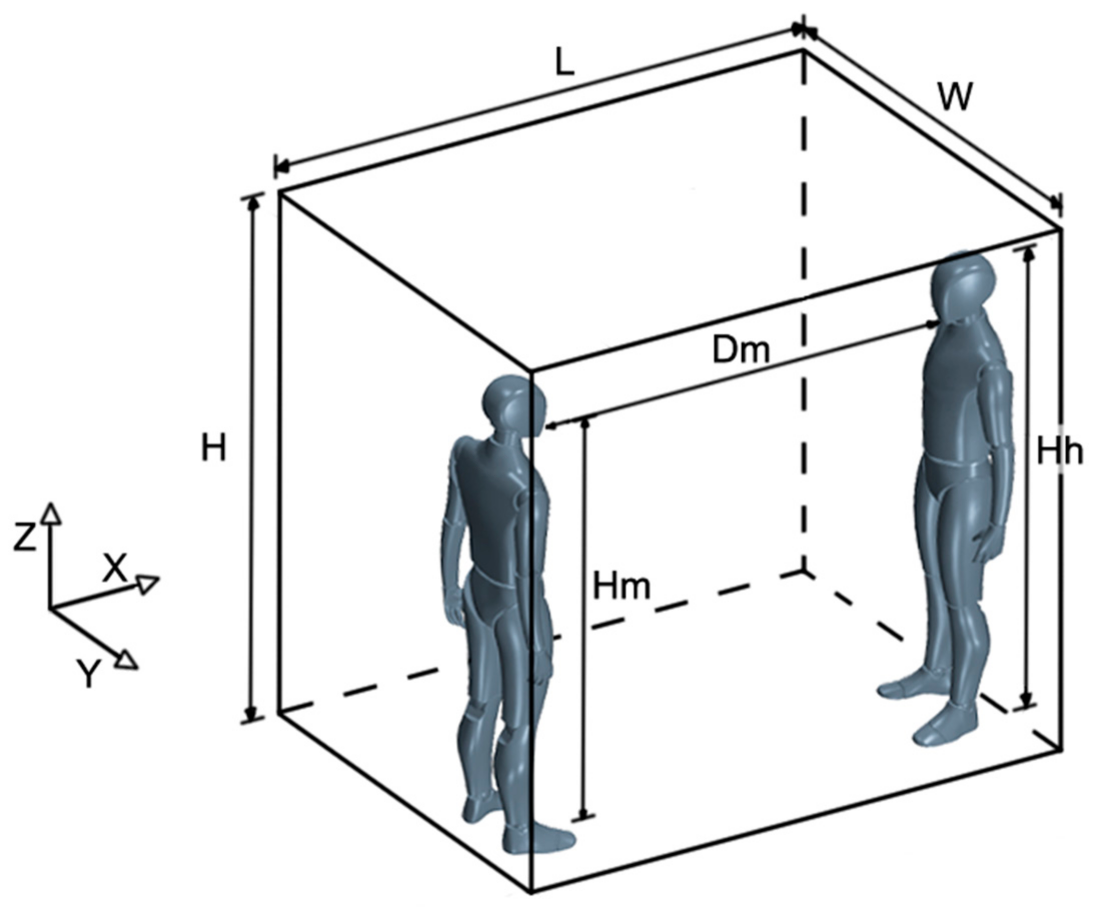
A three-dimensional domain was defined for the current case. The sketch of Figure 1 shows the size of the domain, defined as L = 2.1 m (length), W = 1.2 m (width), and H = 2 m (height). Next to the door of the lift was a human Hh = 1.75 m tall, with its mouth located at Hm = 1.56 m (height) with a mouth opening of Mo = 5 mm and a mouth width of Mw = 40 mm (see Figure 2). This rectangle mouth shape was defined as a velocity surface injector and its velocity values were 8.5, 17.7, and 28 m/s during the first 0.12 s of each simulation. For these velocities, the Reynolds number varied from 4300 in the case of 8.5 m/s inlet velocity to 14,300 in the case of 28 m/s. The total injected saliva mass was 6.7 mg per simulation, in accordance with Zhu et al. [13], at 35 °C. According to van der Reijden et al. [21], human saliva is different according to subject variables, such as if the subject is a smoker or not or if they suffer with diabetes or thirst, among others; however, its viscosity is usually close to that of water. Inside the domain, another human was positioned in the corner in front of the first human at the same plane, at Dm = 1.55 m away. All of the dimensions are shown in Table 1.
The domain was composed of hexahedral cells (526,392 cells), as shown in Figure 3. The mesh was refined close to the mouth and then coarsened gradually in a streamwise direction using a multilevel mesh technique. Five volume controls (VCs) were used for the mesh discretization, each one with different mesh refinement regions. From the finest ones to the coarser ones, the quantity of cells for each VC were VC1 = 173,568, VC2 = 230,928, VC3 = 103,229, VC4 = 12,283, and VC5 = 6384 cells. The most refined zone was near to the mouth. A more refined region close to the mouth was performed, since in this area, the highest turbulences were expected.
A mesh dependency study was carried out to ensure that the numerical solution is independent of the mesh size. Richardson’s extrapolation [22] was used. Three different meshes (fine, medium, and coarse) with mesh sizes h1, h2, and h3, respectively, were used, following the similar study of Aramendia et al. [23]. A mesh refinement ratio of r ≈ 2 was used for the grid dependency study (see Equation (2)).
The axial velocity was measured at a point 14 cm from the mouth downstream. This point was the chosen parameter to control the study. Table 2, Table 3 and Table 4 show the results obtained for the case with an initial cough velocity of 8.5 m/s.
The axial velocities were extrapolated using Equation (3), where p is defined as the accuracy level given by Equation (4).
Grid convergence index (GCI) was used to calculate the discretization error of the solution in the aforementioned three levels of mesh using Equations (5) and (6). According to Roache [24], the smaller the GCI value, the nearer to the asymptotic range of convergence.
Table 3 and Table 4 show the percentage errors of the GCI results for each mesh level. According to these results, the M1 mesh level, which consists of 526,392 cells, was selected to create the numerical model, since the GCI23/rp·GCI12 relationship was near 1.
All of the boundaries were treated as an impermeable wall, including the lift walls, the ground, the ceiling, and both humans. The droplets were set up to stick to the walls. The unique exception was the mouth of the human that coughs, which was set up as a velocity inlet. The conditions inside the elevator were a free stream flow velocity equal to zero, a static pressure of 1 atm, and a static temperature of 21 °C. The walls, ground, and ceiling of the lift were at 18 °C.
2.3. Numerical Set-Up
The equations for the continuous phase were expressed in Eulerian form. Instead, the Lagrangian description permitted solving the dispersed phase while it crossed the computational domain. In a Lagrangian field, parcels (particle-like elements) represent the real quantity of droplets in the dispersed phase and are inserted in the computational domain by injectors. A surface injector was used to model the droplets expelled by the mouth. The air in the region near to the walls benefits the presence of turbulent eddies, which can lead to an aleatory state of motion. Dbouk et al. [7] also suggested that when saliva droplets interact with the air and start dispersing, they convert into droplet nuclei and the turbulence and evaporation disturb the reached dispersion distance. The size distribution and traveled space of its cores can greatly impact to infection risk indoor. That turbulence, that influences the trajectory of the saliva particles and their wide dispersion, has been introduced in our study using the turbulence Reynolds-averaged Navier–Stokes (RANS) equations with k-ω Shear Stress Transport (SST) turbulence model, developed by Menter [25]. The influence of the gravity force was taken into account.
A particle in a turbulent flow experiments with arbitrary velocity gradients to which it responds, depending on its inertia. When a parcel gets into a turbulent carrier flow, it experiments with a random path in terms of interaction with turbulent flow. Each parcel experiments with its own path. Turbulent dispersion has been modeled by a stochastic approach according to the work of Gosman and Ioannides [26]. This study took into account the effect of instantaneous velocity changes on a droplet.
The dissipation length scale () is the characteristic size of the sampled eddy. Equation (7) provides the value for fully developed duct flows.
where L is the width of the outer ring. Once the dissipation length scale is known, the turbulent dissipation rate can be calculated with Equation (8).
where is an empirical constant of the turbulent model; its value is 0.09 and k is the turbulent kinetic energy.
Furthermore, the velocity of the dispersed droplets was calculated using the Newton’s second [7]:
where is the droplet’s mass, is the droplet’s velocity, () are the forces acting on the droplet and B represents the external force of gravity.
The drag force, which solves the force on a droplet due to its velocity in relation to the continuous phase, is described by Equation (10). The drag coefficient (CD) is a function of the small-scale flow characteristics in terms of individual droplets. These features are impractical to resolve spatially the spreading of droplets, and so the usual exercise is to obtain the drag coefficient from interpolations. In the current study, the Schiller–Naumann correlation, usable for liquid droplets, was employed:
where is the projected area of the particle, is the particle slip velocity and is the density of the continuous phase.
In Equation (11), is the Sherwood number, is the Schmidt number, the potential function driving the evaporation, and t is time. Meanwhile, in Equation (12), is the particle relaxation time, is the density for a particle, µ is the dynamic viscosity of the carrier phase, and the diameter of the droplet.
The key to preventing the virus from spreading is the time that saliva droplets, which are exhaled from the mouth, take to evaporate. The saturation pressure and critical temperature are two properties that determinate the vaporization rate, which are added to the material properties of the Lagrangian phases. Therefore, the relative humidity as an initial condition was determined by the Antoine equation [9], which is available for the saturation pressure. It is based on the logarithm of the ratio /, defined by Equation (13):
where is 1 bar, T is temperature (K), n is the base of the logarithm, and A, B, and C are the equation coefficients.
During evaporation, the size of droplets varies. The model of evaporation used in this work was the so-called quasi-steady evaporation model [9]. This model allows droplet particles to lose mass through evaporation. Besides the driving force, this model is determined by Sherwood´s number regarding droplets. The rate of change of a droplet’s mass due to quasi-steady evaporation is calculated by Equation (14):
where B is the Spalding transfer number, * is the mass transfer conductance and is the droplet surface area.
Focusing on heat transfer, the correlation used was the Ranz–Marshall correlation [9]. This correlation is suitable for spherical particles up to Re ≈ 5000, and is applied in the evolution of the mass of saliva-only droplet particle due to evaporation. This correlation defines the coefficient of heat transfer as a derivative correlation as a function of the Nusselt number [7].
Moreover, adding the heat transfer emitted as convection and radiation minus the heat transfer emitted as losses provides the enthalpy difference . Thereby, we obtained the evolution of the droplet’s temperature [7]:
where Ap is the droplet’s surface area, is the heat transfer due to convection gained from the surrounding of the particle, is the heat transfer due to radiation gained from the surrounding of the particle and is the heat transfer emitted as radiation
In addition, in order to calculate the interactions between the airflow and the droplets, the two-way coupling model was used. When the particles leave the mouth and interact with the airflow, the particles are distorted and break. This phenomenon was taken into account using the Taylor analogy breakup (TAB) model. Taylor analogy represents the distortion of a droplet as in a damping springmass system; it reflects only the basic mode of oscillation of the particle. In this work, the commercial code STAR-CCM+ v.14.02 (Siemens, London, UK) was used to perform the simulations. The simulations were carried out on a personal server-clustered parallel computer with Intel Xeon © E5-2609 v2 CPU @ 2.5 GHz (16 cores) and 45 GB RAM. The simulations converged into an acceptable residual value, achieved in the fields of velocity, pressure, and turbulence. This research took approximately 29 days for each simulation.
3. Results
3.1. Initial Size Droplet Dispersion
The dispersion of particles of different diameters is represented in Figure 4, along with the time in different rows (0.12 s, 0.25 s 0.5 s, 0.75 s and 1 s) for the different cough velocities, which are shown in the three columns (8.5 m/s, 17.7 m/s and 28 m/s). Regarding the time, 0.12 s refers to the time when the cough ends and all of the particles are inside the domain. In , the most distant particles are at 13 cm, 20 cm and 25 cm for 8.5 m/s, 17.7 m/s and 28 m/s, respectively, from the mouth. At any time, the advance of the heaviest droplets was more pronounced in comparison to the lighter ones, which means that in this short period of time, inertial force plays a primary role.
Figure 5 represents the velocity of the droplets in the first second of the simulation. The results showed how, at the end of the complete cough, 0.12 s, larger particles advanced horizontally from the mouth, due to the inertial force. Immediately, these particles started falling down due to the gravity force. In , the initial vertical position of the 100 µm particles was 1.55 m (the mouth height), which means that the gravity force did not have a strong effect at first. In , the 100 µm particles fall 22 cm independently of the initial cough velocity. Furthermore, this concentration of these large particles was volumetrically constant along the different velocities. On the contrary, particles smaller than 50 µm suffered Brownian movements governed by the turbulence of the cough. Although they continued in a horizontal path in the first instance following the cough, the path changed rapidly, and in , these droplets started to disperse vertically according to the created turbulence. Some of these particles, particularly those smaller than 30 µm, reached heights within of 1.65 m, 1.73 m and 1.77 m for the initial velocities of 8.5 m/s, 17.7 m/s and 28 m/s, respectively. As mentioned above, this deviation in height was due to the generated turbulence. This turbulence evolution can be observed in Figure 5. The velocity fields are shown in a cross-section plane of the computational domain. Note that at higher velocities values, the turbulence was higher as well. This turbulence generated greater dispersion of the small droplets located at higher positions. The smallest droplets tried to travel horizontally with a short angle deviation upward. Instead, there was a greater concentration of larger droplets—which were more influenced by the gravity force—at lower initial velocities. Figure 5 also illustrates clearly the distances reached horizontally. It is noticeable how the larger particles did not deviate too far in terms of distance from the ending of the cough and the longitude in the first second. The increase in distance was approximately 4–6 cm for the 100 µm droplets. In the case of smaller droplets (<50 µm), the distance traveled was more considerable. In the case of an initial velocity of 8.5 m/s, the maximum distance in the first second was approximately 0.31 cm from the mouth; meanwhile, it was 0.41 cm in the case of 17.7 m/s and 0.54 cm in the case of 28 m/s. Thus, it is clear that drag force plays a primary role in decelerating the velocity of droplets and stopping them.
3.2. Effect of the Evaporation on the Size and Quantity of Droplets
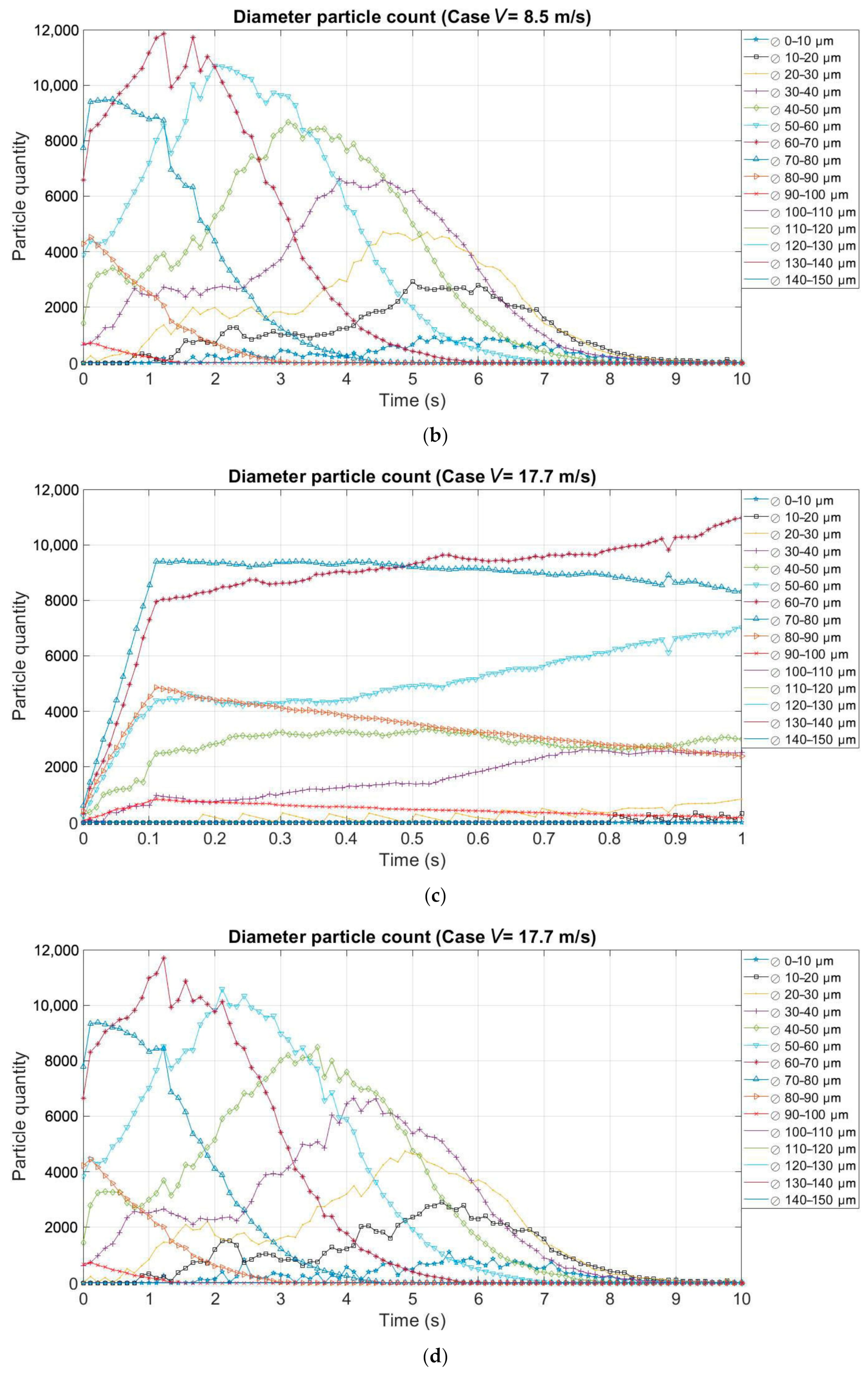
In the first instance following the cough, the most representative times of the evaporation behavior of droplets are demonstrated. Figure 6 shows plots of the different counts of particles of different diameters in ranges of 10 µm from 0 to 150 µm. It is possible to observe the evaporation rates, along with the time and the reduction in droplets. During the cough action, in the first 120 ms, the most frequent diameter range was 70 µm to 80 µm, reaching a value of 9400 droplets. After this, this range of droplets quantity slowly decreased. This decay means an increase in the quantity of 60–70 µm droplets, which became the most frequent size range from 0.5 to 2 s. Overall, the evaporation of larger droplets generated a transition from this size range to consecutively smaller ranges. These evaporation rates did not deviate depending of cough velocity. Some differences in quantities were visible, but not in terms of the most frequent ranges or time.
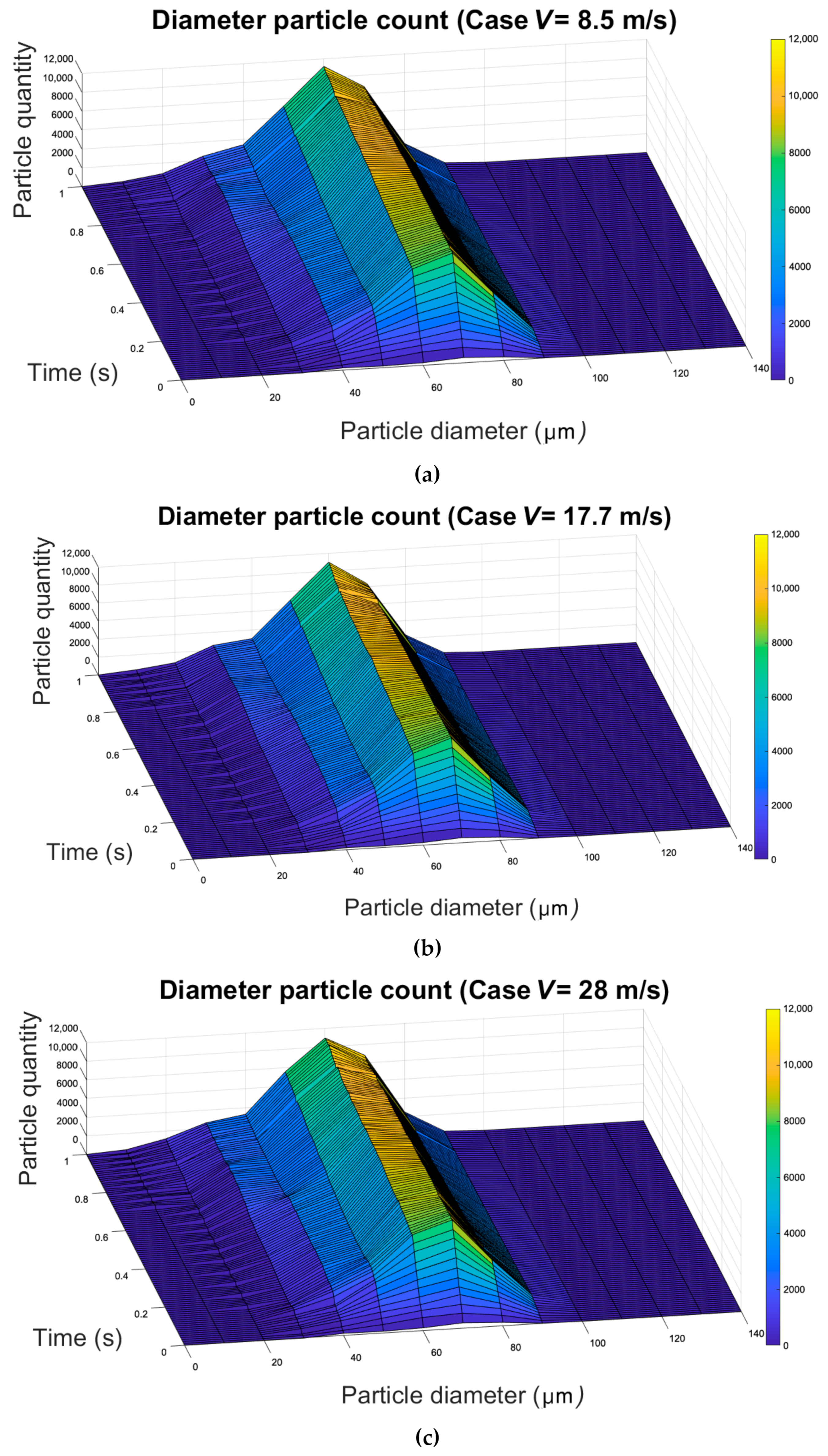
At first (before reaching 1 s), the rise in the number of 60–70 µm particles demonstrated a similar shape as that of the 50–60 µm particles, the latter being a minor value. In general, all of the sizes between 70 and 100 µm suffered a decreasing trend in the number of droplets with a similar gradient. On the contrary, the number of 50–70 µm droplets increased during the first second. This means that besides evaporation, there were also a considerable number of larger broken droplets. Comparing the lines of the 30–40 µm and 40–50 µm particles, a difference between the number and gradients is observable, being the 40–50 µm line more irregular. During the first 0.12 s, in contrast to the 30–40 µm range, which tended to increase in a more continuous way, the 40–50 µm size range showed an irregular increasing pattern, after which it presented a decreasing trend. The reason is that the large broken droplets tended to result in particles of 40–50 µm in size during the first turbulences. Afterward, they started evaporating. Later, at times of 0.7–0.8 s, droplets smaller than 0–30 µm appeared with an irregular tendency of being very low in number less than 500, which means that due to evaporation, they disappeared quickly. Appendix A shows the three-dimensional distribution of the number of particles during the first second for each velocity case.
In a longer time period (before reaching 10 s), Figure 6 illustrates the whole evaporation transformation. The 50–90 µm droplets showed a continuous increase and a regular decrease. The larger the particle size range, the faster their number reached zero. Meanwhile, the 30–50 µm droplets had a more irregular increase with a regular decrease. This could be due to the breakup of larger droplets, forming more droplets in this size range. Finally, the 0–30 µm droplets had a completely irregular increase, with fewer droplets in the smaller size range, and a fast decay in terms of quantity. This means that the evaporation rate of these particles was very high. In fact, the 0–10 µm particles appeared first in 1.7 s and did not exceed 1000 particles, having a totally irregular evolution over time. In the ninth second, no droplets existed in the domain.
3.3. Spreading of Saliva Droplets
Several countries have imposed a safe social distance of at least 1.5 m between persons. The majority of governments have recommended a 2 m distance. In the latest WHO recommendations, it is advised to maintain a 1 m distance at least in indoors, being the further away, the better. According to Dbouk et al. [7,8], a 2 m distance is safe only when no airflow exists. Busco et al. [9] concluded that the final traveling distance of droplets can be increased by the effect of body mimics. Aliabadi et al. [12] and Zhang et al. [20] studied the effects of different parameters related to the trajectory of droplets.
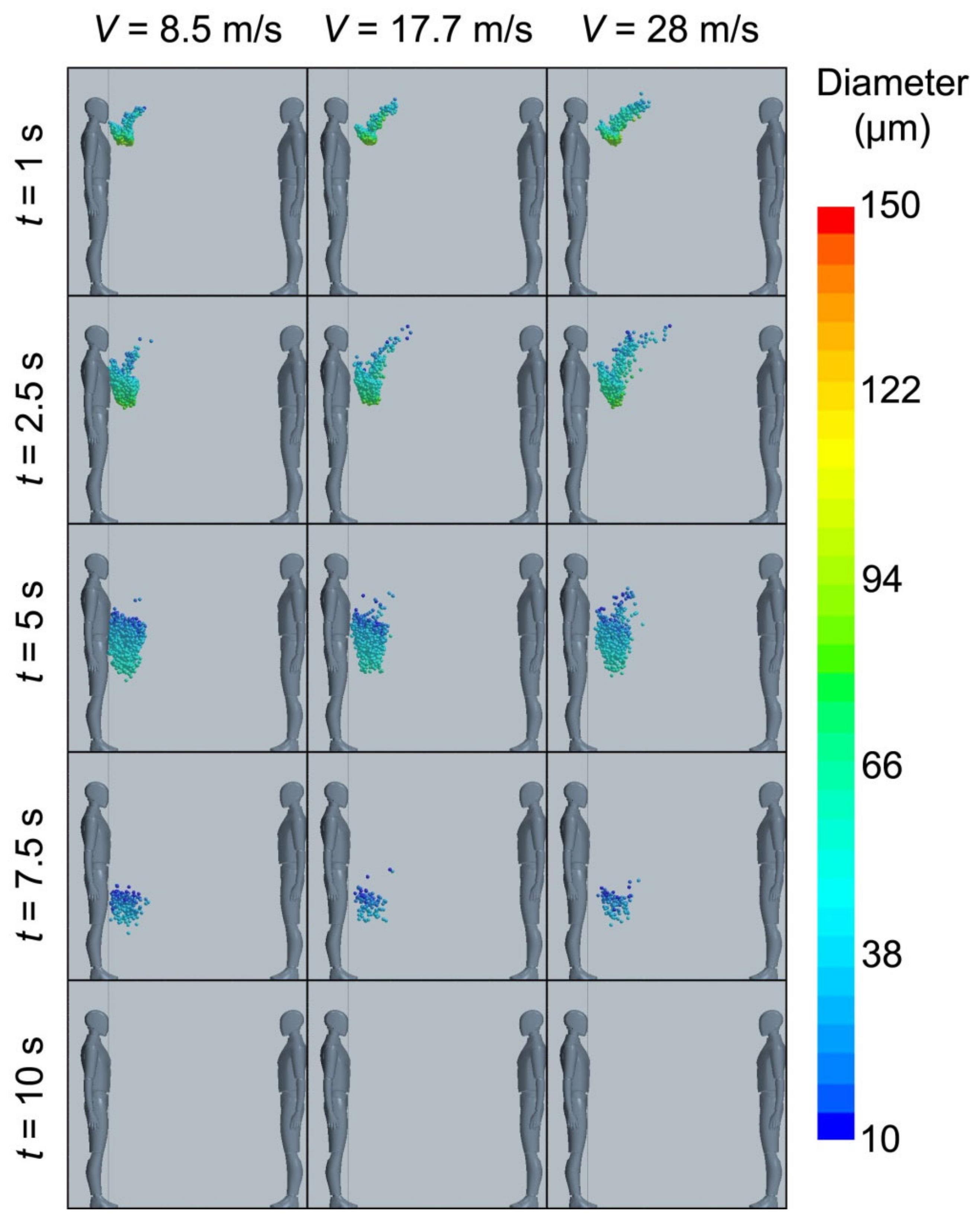
In the current study, the distance reached by the droplets, with a focus on their sizes and the maximum distance traveled in a time interval of 1–10 s, was investigated. To evaluate better the safest distance, a second human at a distance of 1.5 m was introduced into the domain. Figure 7 shows the time-lapsed dispersion for three velocities (8.5 m/s, 17.7 m/s and 28 m/s). The droplet cloud can be defined as V-shaped and more dispersed at higher initial velocity. The larger droplets (the heaviest ones) were situated at the bottom of the cloud, while the lighter ones were located at the top and farther away from the mouth. The bottom of the cloud increased in volume, more homogeneously at lower initial velocities until 5.5 s, when the size star reducing the volume of the cloud due to the complete evaporation of lighter droplets. Evaporation is volumetrically more linear at low velocities. By 5.5 s, the top of the cloud had completely disappeared. At higher velocities, it was more difficult to differentiate the two parts of the cloud. The generated turbulence mixed the droplets and created a moisture bridge, which maintained the top of the cloud for a longer time, being this very dispersed and mixed. By 9 s from the start of the cough, all of the droplets had evaporated before reaching the ground.
4. Conclusions
In this study, a CFD simulation based on Eulerian–Lagrangian models was presented. The domain was a reproduction of an elevator with the following dimensions: 2.1 m in length, 1.2 m in width, and 2 m in height. Inside, two humans were introduced 1.5 m away from one another. One of the human emitted droplets due to a cough, which lasted 0.12 s. This cough was simulated at three air injection velocities: 8.5 m/s, 17.7 m/s and 28 m/s. The distribution of droplets of different sizes is defined by a Rosin–Rammler distribution.
The behavior of the expelled droplets due to a cough was analyzed. The evaporation, mass transfer, turbulence force dispersion, droplet breakup, and phase change were taken into account. The simulation was set up to model a cough and to calculate its evolution for 10 s in an elevator space with two subjects inside.
According to the obtained results, it can be observed how, at the beginning of the cough, particles of <10 µm were not visible, and how droplets of this size range only appeared at nearly 2 s. This phenomenon is due to the evaporation of larger particles, turning them into smaller droplets. According to the achieved results, the dispersion of droplets may vary depending on the exhalation velocity, reaching a maximum distance lengthwise from the mouth of 40 cm, 50 cm and 70 cm for 8.5 m/s, 17.7 m/s and 28 m/s, respectively. Instead, this variable did not affect, or at least only to a small extent, to evaporation behavior. The disappearance of liquid droplets occurred from top to bottom. This is due to small droplets having more buoyancy and evaporating faster than larger ones. The buoyancy and different dissipation ratios of small droplets resulted in a progressive vertical evaporation. First, the small droplets located at mouth height dehydrated. Complete evaporation occurred in order of descending height. In the 9th second, droplets are not present in the domain. Last droplets disappear at a height between 40 and 55 cm from the ground. According to Busco et al. [9], human mimics sneezing related reactions could spread expelled droplets until twice or more than without human mimics. Since a cough is less violent than a sneeze, the emitted droplets achieve shorter distances. In this case, recommended social distance of 1.5 m should be enough to prevent inhalation via infections in calm spaces.
Author Contributions
Conceptualization, S.A.C.; methodology, S.A.C.; software, I.A.; validation, S.A.C., I.A. and U.F.-G.; formal analysis, S.A.C.; investigation, S.A.C. and A.U.-A.; resources, S.A.C.; data curation, S.A.C. and E.Z.; writing—original draft preparation, S.A.C. and A.U.-A.; writing—review and editing, S.A.C. and U.F.-G.; visualization, S.A.C.; supervision, U.F.-G.; project administration, U.F.-G.; funding acquisition, U.F.-G. All authors have read and agreed to the published version of the manuscript.
Funding
The authors appreciate the support to the government of the Basque Country through research programs Grants N. ELKARTEK 20/71 and ELKARTEK 20/78.
Institutional Review Board Statement
Not applicable.
Informed Consent Statement
Not applicable.
Data Availability Statement
The data presented in this study are available on request from the corresponding author.
Acknowledgments
The authors are grateful for the support provided by SGIker of UPV/EHU.
Conflicts of Interest
The authors declare no conflict of interest.
Appendix A
Figure A1.
Different diameters particles quantities during first second from cough start: (a) Case 8.5 m/s; (b) Case 17.7 m/s; (c) Case 28 m/s.
Figure A1.
Different diameters particles quantities during first second from cough start: (a) Case 8.5 m/s; (b) Case 17.7 m/s; (c) Case 28 m/s.
References
- Hadi, A.G.; Kadhom, M.; Hairunisa, N.; Yousif, E. A Review on COVID-19: Origin, Spread, Symptoms, Treatment, and Prevention. Biointerface Res. Appl. Chem. 2020, 10, 7234–7242. [Google Scholar]
- Moriyama, M.; Hugentobler, W.J.; Iwasaki, A. Seasonality of Respiratory Viral Infections. Annu. Rev. Virol. 2020, 7, 83–101. [Google Scholar] [CrossRef]
- Vuorinen, V.; Aarnio, M.; Alava, M.; Alopaeus, V.; Atanasova, N.; Auvinen, M.; Balasubramanian, N.; Bordbar, H.; Erästö, P.; Grande, R.; et al. Modelling Aerosol Transport and Virus Exposure with Numerical Simulations in Relation to SARS-CoV-2 Transmission by Inhalation Indoors. Saf. Sci. 2020, 130, 104866. [Google Scholar] [CrossRef]
- Morawska, L.; Tang, J.W.; Bahnfleth, W.; Bluyssen, P.M.; Boerstra, A.; Buonanno, G.; Cao, J.; Dancer, S.; Floto, A.; Franchimon, F.; et al. How Can Airborne Transmission of COVID-19 Indoors Be Minimised? Environ. Int. 2020, 142, 105832. [Google Scholar] [CrossRef]
- Van Doremalen, N.; Bushmaker, T.; Morris, D.H.; Holbrook, M.G.; Gamble, A.; Williamson, B.N.; Tamin, A.; Harcourt, J.L.; Thornburg, N.J.; Gerber, S.I.; et al. Aerosol and Surface Stability of SARS-CoV-2 as Compared with SARS-CoV-1. N. Engl. J. Med. 2020, 382, 1564–1567. [Google Scholar] [CrossRef]
- Feng, Y.; Marchal, T.; Sperry, T.; Yi, H. Influence of Wind and Relative Humidity on the Social Distancing Effectiveness to Prevent COVID-19 Airborne Transmission: A Numerical Study. J. Aerosol Sci. 2020, 147, 105585. [Google Scholar] [CrossRef]
- Dbouk, T.; Drikakis, D. On Coughing and Airborne Droplet Transmission to Humans. Phys. Fluids 2020, 32, 53310. [Google Scholar] [CrossRef]
- Dbouk, T.; Drikakis, D. On Respiratory Droplets and Face Masks. Phys. Fluids 2020, 32, 63303. [Google Scholar] [CrossRef]
- Busco, G.; Yang, S.R.; Seo, J.; Hassan, Y.A. Sneezing and Asymptomatic Virus Transmission. Phys. Fluids 2020, 32, 73309. [Google Scholar] [CrossRef]
- Asadi, S.; Wexler, A.S.; Cappa, C.D.; Barreda, S.; Bouvier, N.M.; Ristenpart, W.D. Aerosol Emission and Superemission during Human Speech Increase with Voice Loudness. Sci. Rep. 2019, 9, 2348. [Google Scholar] [CrossRef] [PubMed] [Green Version]
- Yang, X.; Ou, C.; Yang, H.; Liu, L.; Song, T.; Kang, M.; Lin, H.; Hang, J. Transmission of Pathogen-Laden Expiratory Droplets in a Coach Bus. J. Hazard. Mater. 2020, 397, 122609. [Google Scholar] [CrossRef]
- Aliabadi, A.A.; Rogak, S.N.; Green, S.I.; Bartlett, K.H. CFD Simulation of Human Coughs and Sneezes: A Study in Droplet Dispersion, Heat, and Mass Transfer. In Proceedings of the Fluid Flow, Heat Transfer and Thermal Systems, Parts A and B, ASMEDC, Vancouver, BC, Canada, 1 January 2010; pp. 1051–1060. [Google Scholar]
- Zhu, S.; Kato, S.; Yang, J.-H. Study on Transport Characteristics of Saliva Droplets Produced by Coughing in a Calm Indoor Environment. Build. Environ. 2006, 41, 1691–1702. [Google Scholar] [CrossRef]
- Wang, B.; Zhang, A.; Sun, J.L.; Liu, H.; Hu, J.; Xu, L.X. Study of SARS Transmission Via Liquid Droplets in Air. J. Biomech. Eng. 2005, 127, 32–38. [Google Scholar] [CrossRef]
- Shao, S.; Zhou, D.; He, R.; Li, J.; Zou, S.; Mallery, K.; Kumar, S.; Yang, S.; Hong, J. Risk Assessment of Airborne Transmission of COVID-19 by Asymptomatic Individuals under Different Practical Settings. J. Aerosol Sci. 2021, 151, 105661. [Google Scholar] [CrossRef] [PubMed]
- Rahiminejad, M.; Haghighi, A.; Dastan, A.; Abouali, O.; Farid, M.; Ahmadi, G. Computer Simulations of Pressure and Velocity Fields in a Human Upper Airway during Sneezing. Comput. Biol. Med. 2016, 71, 115–127. [Google Scholar] [CrossRef] [PubMed]
- Duguid, J.P. The Size and the Duration of Air-Carriage of Respiratory Droplets and Droplet-Nuclei. Epidemiol. Infect. 1946, 44, 471–479. [Google Scholar] [CrossRef] [Green Version]
- Xie, X.; Li, Y.; Sun, H.; Liu, L. Exhaled Droplets Due to Talking and Coughing. J. R. Soc. Interface 2009, 6 (Suppl. 6), S703–S714. [Google Scholar] [CrossRef] [Green Version]
- VanSciver, M.; Miller, S.; Hertzberg, J. Particle Image Velocimetry of Human Cough. Aerosol Sci. Technol. 2011, 45, 415–422. [Google Scholar] [CrossRef]
- Zhang, Y.; Feng, G.; Bi, Y.; Cai, Y.; Zhang, Z.; Cao, G. Distribution of Droplet Aerosols Generated by Mouth Coughing and Nose Breathing in an Air-Conditioned Room. Sustain. Cities Soc. 2019, 51, 101721. [Google Scholar] [CrossRef]
- Van der Reijden, W.A.; Veerman, E.C.I.; Nieuw Amerongen, A.V. Shear Rate Dependent Viscoelastic Behavior of Human Glandular Salivas. BIR 1993, 30, 141–152. [Google Scholar] [CrossRef]
- Richardson, L.F.; Gaunt, J.A. VIII. The deferred approach to the limit. Philos. Trans. R. Soc. Lond. 1927, 226, 299–361. [Google Scholar]
- Aramendia, I.; Fernandez-Gamiz, U.; Lopez-Arraiza, A.; Rey-Santano, C.; Mielgo, V.; Basterretxea, F.; Sancho, J.; Gomez-Solaetxe, M. Experimental and Numerical Modeling of Aerosol Delivery for Preterm Infants. Int. J. Environ. Res. Public Health 2018, 15, 423. [Google Scholar] [CrossRef] [PubMed] [Green Version]
- Roache, P.J. Perspective: A Method for Uniform Reporting of Grid Refinement Studies. J. Fluids Eng. 1994, 116, 405–413. [Google Scholar] [CrossRef]
- Menter, F.R. Two-Equation Eddy-Viscosity Turbulence Models for Engineering Applications. AIAA J. 1994, 32, 1598–1605. [Google Scholar] [CrossRef] [Green Version]
- Gosman, A.D.; Ioannides, E. Aspects of Computer Simulation of Liquid-Fueled Combustors. J. Energy 1983, 7, 482–490. [Google Scholar] [CrossRef]
Figure 1.
Size and layout of the computational domain. L, length; W, width; H, height; Dm, distance between mouths; Hm, mouth height; Hh, human height.
Figure 1.
Size and layout of the computational domain. L, length; W, width; H, height; Dm, distance between mouths; Hm, mouth height; Hh, human height.

Figure 2.
Case details: (a) Mouth location and (b) mouth dimensions. Mo, mouth opening; Mw, mouth width.
Figure 2.
Case details: (a) Mouth location and (b) mouth dimensions. Mo, mouth opening; Mw, mouth width.
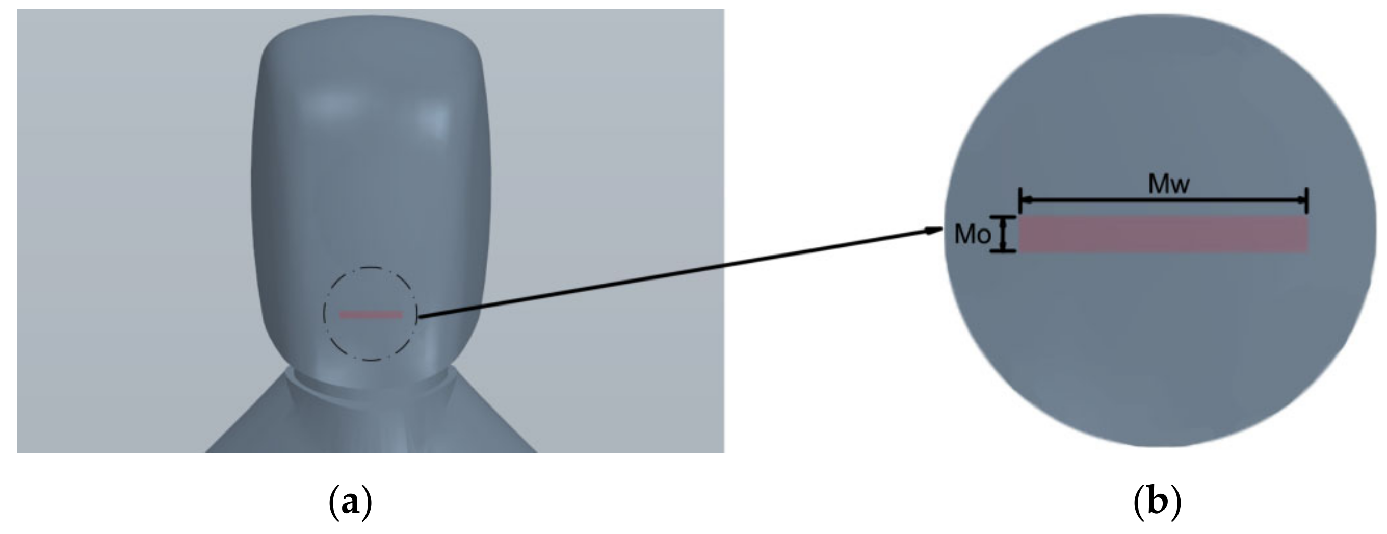
Figure 3.
Mesh distribution in the domain (526,392 cells). VC, volume control.
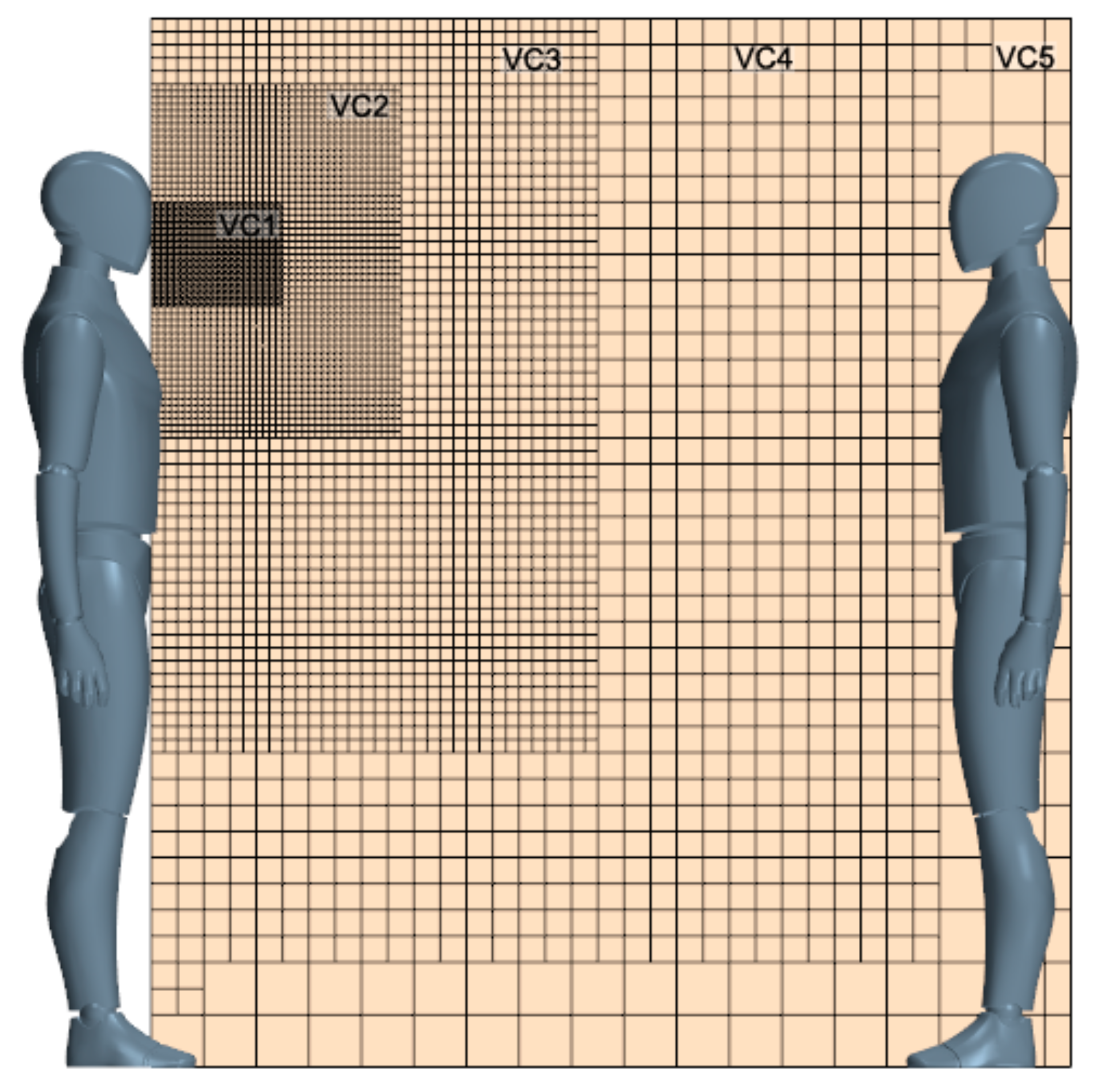
Figure 4.
The diameters of the droplets and their positions in a time interval from 0.03 to 0.15 s. The columns represent the velocity values, which are 8.5 m/s, 17.7 m/s and 28 m/s. The time values are arranged across rows from top to bottom: From 0.03 to 0.15 s, with 0.3 s time intervals.
Figure 4.
The diameters of the droplets and their positions in a time interval from 0.03 to 0.15 s. The columns represent the velocity values, which are 8.5 m/s, 17.7 m/s and 28 m/s. The time values are arranged across rows from top to bottom: From 0.03 to 0.15 s, with 0.3 s time intervals.
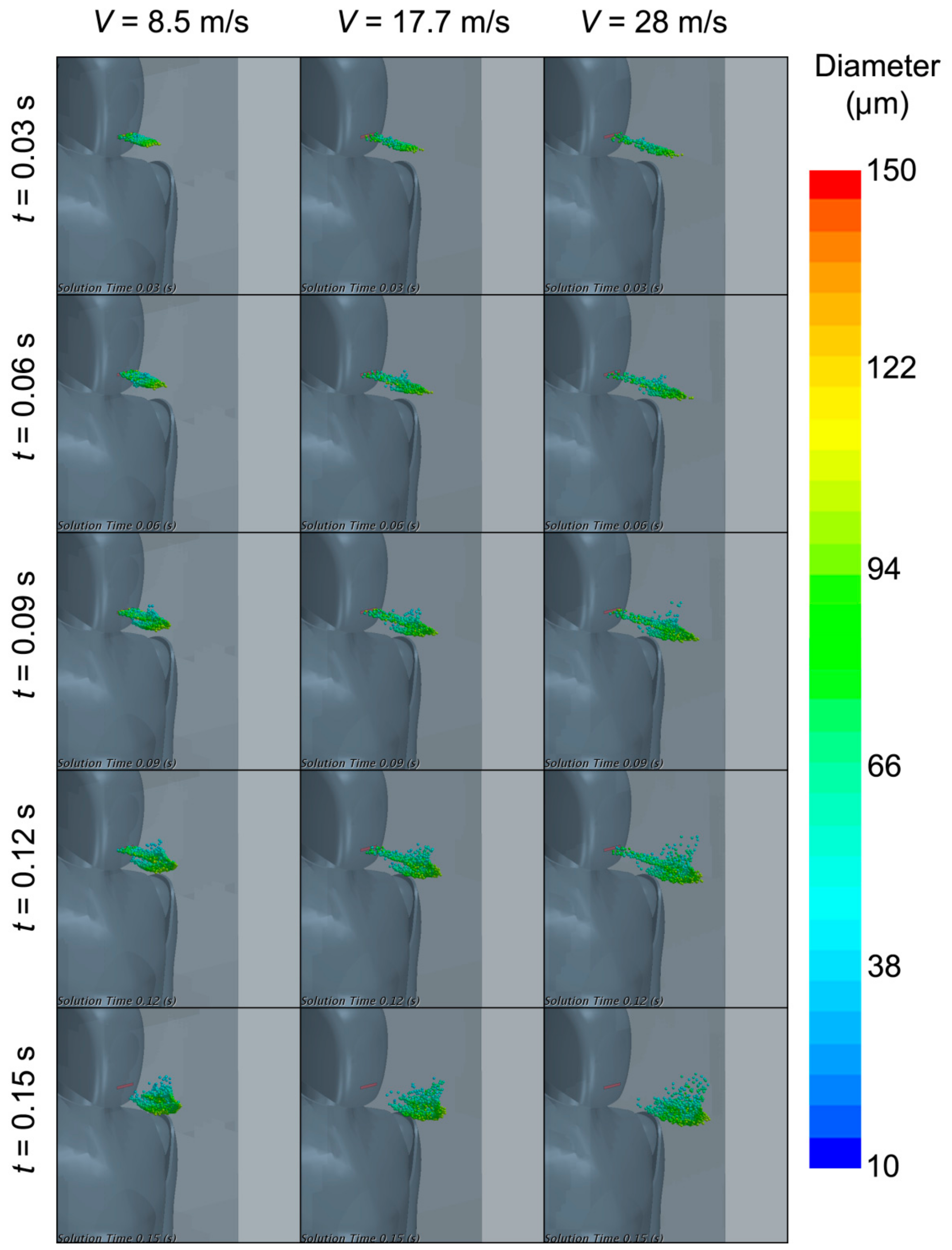
Figure 5.
Initial droplets distribution in a time interval from 0.12 s to 1 s. The rows show the time values: 0.12 s, 0.25 s, 0.5 Scheme 0 s and 1 s. The velocity values are arranged in the columns, from left to right: 8.5 m/s, 17.7 m/s and 28 m/s.
Figure 5.
Initial droplets distribution in a time interval from 0.12 s to 1 s. The rows show the time values: 0.12 s, 0.25 s, 0.5 Scheme 0 s and 1 s. The velocity values are arranged in the columns, from left to right: 8.5 m/s, 17.7 m/s and 28 m/s.
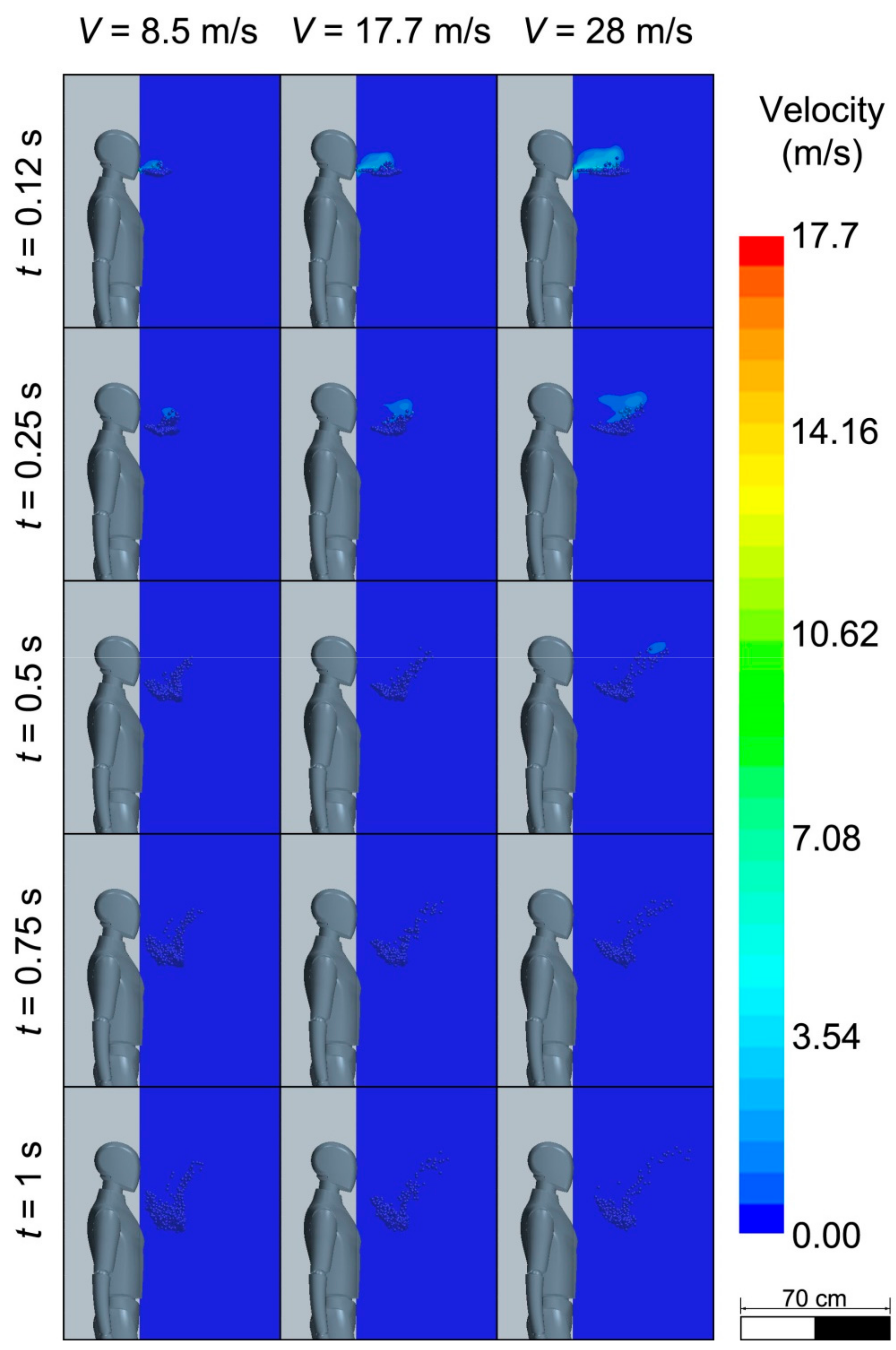
Figure 6.
The distribution of droplets of different sizes over time: (a) 8.5 m/s in the 0–1 s range; (b) 8.5 m/s in the 0–10 s range; (c) 17.7 m/s in the 0–1 s range; (d) 17.7 m/s in the 0–10 s range; (e) 28 m/s in the 0–1 s range; (f) 28 m/s in the 0–10 s range.
Figure 6.
The distribution of droplets of different sizes over time: (a) 8.5 m/s in the 0–1 s range; (b) 8.5 m/s in the 0–10 s range; (c) 17.7 m/s in the 0–1 s range; (d) 17.7 m/s in the 0–10 s range; (e) 28 m/s in the 0–1 s range; (f) 28 m/s in the 0–10 s range.
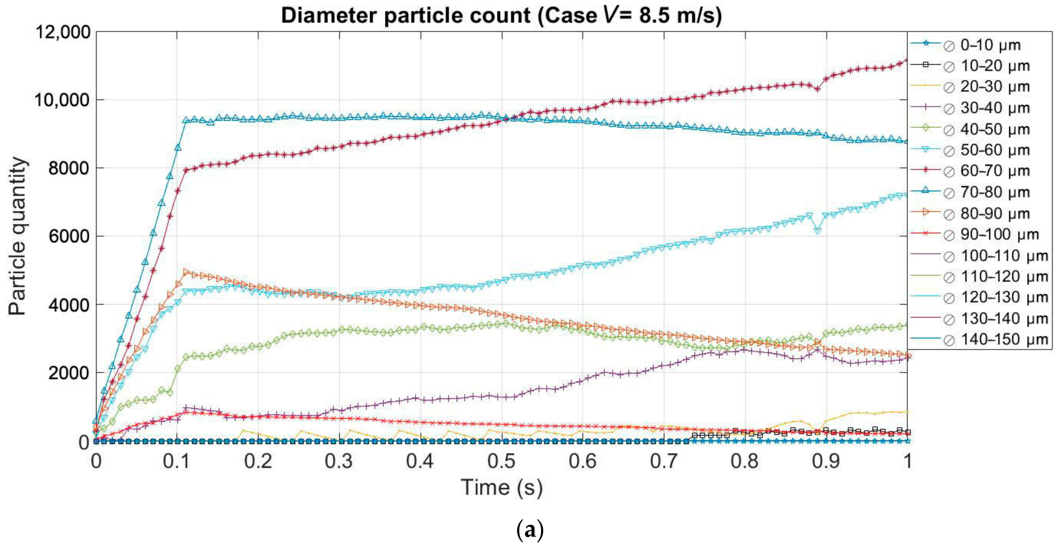

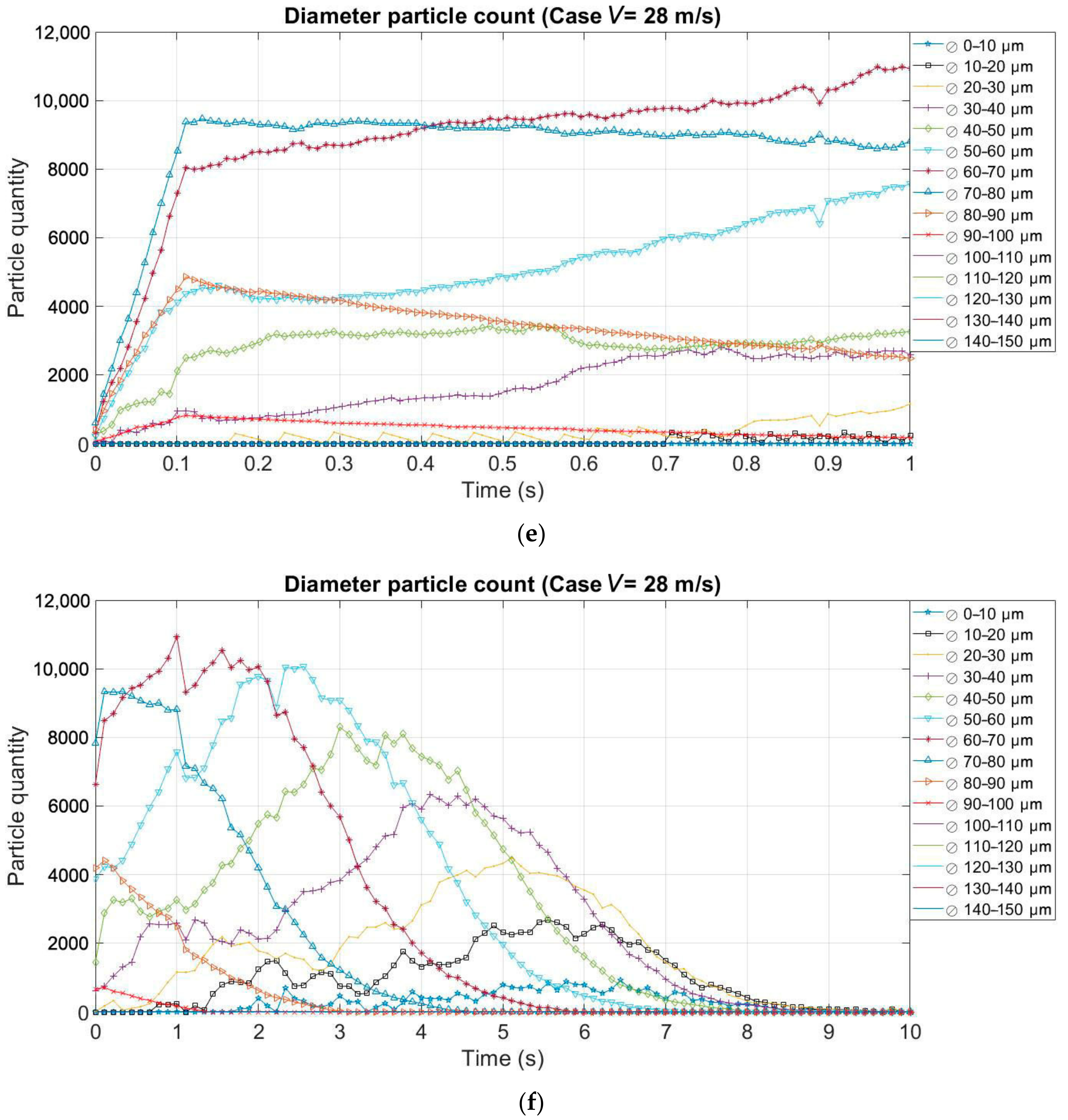
Figure 7.
The diameter of the droplets and their positions in a time interval of 1–10 s. The rows represent the time values: 0.12 s, 0.25 s, 0.5 s, 0.75 s and 1 s. The velocity values are arranged in columns, from left to right: 8.5 m/s, 17.7 m/s and 28 m/s.
Figure 7.
The diameter of the droplets and their positions in a time interval of 1–10 s. The rows represent the time values: 0.12 s, 0.25 s, 0.5 s, 0.75 s and 1 s. The velocity values are arranged in columns, from left to right: 8.5 m/s, 17.7 m/s and 28 m/s.


Table 1.
Computational domain measurements.
| Notation | Meaning | Value |
|---|---|---|
| H | Height | 2 m |
| L | Length | 2.1 m |
| W | Width | 1.2 m |
| Hh | Human height | 1.75 m |
| Hm | Mouth height | 1.56 m |
| Dm | Distance between mouths | 1.55 m |
| Mo | Mouth opening | 5 mm |
| Mw | Mouth width | 40 mm |
Table 2.
Axial velocities of the selected point for each mesh level.
| Mesh | Number of Cells | Vaxial (m/s) |
|---|---|---|
| M1 | 526,392 | 5.62 |
| M2 | 263,196 | 5.45 |
| M3 | 131,598 | 4.98 |
Table 3.
Errors achieved for each mesh level.
| Mesh Level | Vaxial (m/s) | Error (%) |
|---|---|---|
| (Vaxial)h=0 (m/s) | 5.72 | |
| M1 | 5.62 | 1.78 |
| M2 | 5.45 | 4.82 |
| M3 | 4.98 | 13.03 |
Table 4.
Grid convergence index (GCI) results.
| Grid Convergence Index | Domain |
|---|---|
| GCI12 (%) | 2.34 |
| GCI23 (%) | 6.93 |
| GCI23/rpGCI12 (-) | 1.09 |
Publisher’s Note: MDPI stays neutral with regard to jurisdictional claims in published maps and institutional affiliations. |
© 2021 by the authors. Licensee MDPI, Basel, Switzerland. This article is an open access article distributed under the terms and conditions of the Creative Commons Attribution (CC BY) license (http://creativecommons.org/licenses/by/4.0/).
Share and Cite
MDPI and ACS Style
Chillón, S.A.; Ugarte-Anero, A.; Aramendia, I.; Fernandez-Gamiz, U.; Zulueta, E. Numerical Modeling of the Spread of Cough Saliva Droplets in a Calm Confined Space. Mathematics 2021, 9, 574. https://doi.org/10.3390/math9050574
AMA Style
Chillón SA, Ugarte-Anero A, Aramendia I, Fernandez-Gamiz U, Zulueta E. Numerical Modeling of the Spread of Cough Saliva Droplets in a Calm Confined Space. Mathematics. 2021; 9(5):574. https://doi.org/10.3390/math9050574
Chicago/Turabian StyleChillón, Sergio A., Ainara Ugarte-Anero, Iñigo Aramendia, Unai Fernandez-Gamiz, and Ekaitz Zulueta. 2021. "Numerical Modeling of the Spread of Cough Saliva Droplets in a Calm Confined Space" Mathematics 9, no. 5: 574. https://doi.org/10.3390/math9050574
Note that from the first issue of 2016, this journal uses article numbers instead of page numbers. See further details here.