
Parametric Estimation of Diffusion Processes: A Review and Comparative Study


Department of Statistics, Mathematical Analysis and Optimization, University of Santiago de Compostela, Rúa de Lope Gómez de Marzoa s/n, 15705 Santiago de Compostela, Spain
*
Author to whom correspondence should be addressed.
Mathematics 2021, 9(8), 859; https://doi.org/10.3390/math9080859
Submission received: 8 March 2021
/
Revised: 9 April 2021
/
Accepted: 12 April 2021
/
Published: 14 April 2021
(This article belongs to the Special Issue Financial Modeling)
Abstract
:This paper provides an in-depth review about parametric estimation methods for stationary stochastic differential equations (SDEs) driven by Wiener noise with discrete time observations. The short-term interest rate dynamics are commonly described by continuous-time diffusion processes, whose parameters are subject to estimation bias, as data are highly persistent, and discretization bias, as data are discretely sampled despite the continuous-time nature of the model. To assess the role of persistence and the impact of sampling frequency on the estimation, we conducted a simulation study under different settings to compare the performance of the procedures and illustrate the finite sample behavior. To complete the survey, an application of the procedures to real data is provided.
1. Introduction
Diffusion processes described by stochastic differential equations (SDE) are frequently applied in physical, biological and financial fields to model dynamical systems with a disturbance term. Its use in mathematical finance for modeling the evolution of important economic variables, such as the interest rate, has been increasingly important over the last decades. The need to develop the analysis of the term structure of interest rates in a stochastic environment emerges as a consequence of market turbulence throughout the seventies. New theories of the term structure of interest rate based on pricing models in absence of arbitrage under stochastic environment were emerging: Merton [1] used the interest rate in option pricing modeling it as a stochastic process. Subsequently, Black and Scholes [2] had an important impact on arbitrage models of the term structure of interest rates, as shown in [3,4,5,6,7]. In these models, the interest rate is the solution of the stochastic differential equation, therefore we can use the framework of Markov processes theory for its analytical treatment. The continuous time paradigm proves to be an especially useful tool, but the continuous time nature of the model does complicate the estimation of the parameters because available data are sampled in discrete time. Thus, parameter estimates are subject to discretization bias together with estimation bias and this issues have been addressed using different estimation methods. The finite sample bias is especially acute when the process is highly persistent, such as time series of interest rates, and alters the valuation of derivatives since short term interest rate models are used to price these instruments [8].
We consider the SDE defined in a filtered probability space , where is a nonempty set, is a -algebra of subsets of and is a probability measure, . We will focus on parametric time-homogeneous stochastic differential equations, where is an Itô process,
with , a -adapted standard Wiener process and an unknown parameter vector such that with d a positive integer and a compact set. We assume the knowledge of the drift and diffusion functions parametric structure, and , respectively, where none is time dependent. Jump-diffusions and fractional Brownian motion or Lévy-driven SDEs are out of the scope of this review.
A parametric specification of (1) that encloses different interest rate models is the Chan–Karolyi–Longstaff–Sanders (CKLS) model proposed in [6], given by
which is a mean-reverting process that allows the conditional mean and variance to depend on the interest rate level X. The drift parameter is the long-term mean and is the rate of reversion, while the diffusion parameter is the volatility and is the proportional volatility exponent that measures the sensitivity of the volatility regarding the process in time t. This model generalizes prior interest rate models by imposing restrictions on the parameters. When is 0 or —which yields the Vasicek [3] and CIR [5] model, respectively—the process is tractable and admits an analytical solution.
In this article, we consider SDEs with deterministic volatility function, though current option pricing literature withdraws the constant volatility assumption and adopts instead a stochastic volatility framework. Nevertheless, the issues addressed here are inherited by stochastic volatility models and the estimation methods can be extended to SDEs with volatility described by a stochastic process. Furthermore, models based on the Vasicek process are still used in the financial market (see, e.g., [9] or [10]) and new estimation procedures are being proposed for jump-diffusions [11] or Lévy-driven processes [12].
Several studies of estimation methods for diffusion processes can be found in the literature, see [13] for a theoretical comparison or [14] for a more practical approach. In [15], a comparative study of different discretization methods and moment-based estimation is carried out, while [16] focused on simulation-based approaches. The aim of this paper is to complement these comparative studies extending the evaluation of the finite sample performance to different settings—near unit-root time series, various degrees of persistence without changes in the marginal density or different sampling intervals and observation times—whose impact on estimation have been hinted at in the financial literature. The methods here considered are maximum likelihood estimation, local linearization [17,18], Hermite polynomial expansion [19], Kalman filter [20], Markov Chain Monte Carlo [21,22] and generalized method of moments [6,23]. The procedures are provided in the companion estsde R package [24], implemented in C and C++ for the sake of efficiency.
The sections are organized as follows: Section 2 provides an outline of the estimation methods, Section 3 designs the Monte Carlo experiment and discusses the finite sample performance of the procedures. Real data applications to interest rate series are presented in Section 4 and conclusions are drawn in Section 5. Tabulated simulation results are deferred to Appendix A.
2. Estimation Methods
The unique strong solution of the SDE in (1),
exist under the assumptions that both drift and volatility functions satisfy global Lipschitz continuous and growth conditions (see, e.g., [25]):
Assumption 1
(Global Lipschitz). For all there exist a constant independent of θ such that
Assumption 2
(Linear growth). For all there exist a constant independent of θ such that
Although the model is formulated in continuous time, data are registered in discrete time points. In this regard, for the estimation of the continuous time model parameters we should consider a discrete version of it. The observation scheme assumed is the fixed-Δ scheme, in which the time step between two consecutive observations is fixed and the sample size increases, as well as the time interval . One of the most used approximation schemes is the Euler–Maruyama method [26]: given an Itô process , solution of the SDE in (1) with initial value and the discretization of the time interval , , the Euler–Maruyama approximation of X is a continuous stochastic process that satisfies the iterative scheme
with , and .
In the remainder of this section, we provide an outline of the procedures and their implementation to estimate the unknown parameter vector . The methods described fall into two categories: likelihood-based and method of moments. The method of moments provides estimates by matching population and sample moments and minimizing a quadratic form, hence we assume that the moment conditions of are bounded:
Assumption 3
(Bounded moments). For all , all order k moments of the diffusion process exist and are such that
The maximum likelihood (ML) estimates are yielded by different methods: exact and discrete (piecewise constant or linear approximations) ML, univariate Hermite expansion of the transition function, filtering algorithm (linear quadratic estimation) and Bayesian approach.
2.1. Exact Maximum Likelihood
As is a Markov process, we can obtain the likelihood function of the discrete process using Bayes’ rule,
where denotes the transition density function associated to the parametric diffusion model, with unknown parameter . If the parametric form of the model that generates the observations is known, we can use a maximum likelihood method, so that the maximum likelihood estimator (MLE) of the true parameter is
where is the log-likelihood function. This estimation method can seldom be used with diffusion processes, as few models have a closed-form solution, e.g., [2,3,5]. As a consequence, new procedures have been proposed in the ML framework based on different approximations of the transition density function.
2.2. Discrete Maximum Likelihood
Discrete time likelihood (also known as pseudo-likelihood) methods emerge as an alternative approach to approximate the unknown transition density of SDEs, where the diffusion model is discretized with a certain numerical scheme, when exact maximum likelihood is unfeasible. In some cases, analytical expressions for the parameters estimates can be obtained, otherwise a numerical optimization routine is needed to maximize (minimize) the (negative) log-likelihood. Several algorithms have been proposed to approximate SDEs (see, e.g., [18,27,28]), here we briefly detail two of them.
2.2.1. Euler Method
To estimate the model we can use an approximation scheme, such as the Euler–Maruyama [26] method. With this method we do not approximate the transition density directly, instead the trajectory of the process is approximated so that we can use the likelihood of the discretized version of the model, given by
where are i.i.d. and . Therefore, the estimation with the Euler–Maruyama method [29] proceeds as if the observations follow a Gaussian distribution, with mean the drift function and standard deviation the diffusion function. Thus, the transition density is given by
The implementation of this method is straightforward, however, Euler-type schemes depend on the sampling interval and introduce discretization bias in the estimates, although they converge to exact ML estimates as . Departures from Gaussian distribution can also increase bias since the Euler scheme increments are conditionally Gaussian.
2.2.2. Local Linearization
While the Euler–Maruyama approximation method restricts coefficients of the drift and diffusion terms to be piecewise constant, the local linearization instead uses a linear approximation. Considering the SDE
where is assumed constant, the local linearization (LL) method developed in [17,18] is an approximation method by which the drift function is locally approximated by a linear function of (no expansion is required for the diffusion function, as it is constant). The numerical scheme is based on the local linearization of the SDE’s drift coefficient by means of a truncated Itô–Taylor expansion. The process discretized by the LL method is
where
and .
The linear function approximates the drift function , with constant in the interval . Given that the stochastic integral is a Gaussian random variable, the transition density for given is indeed Gaussian. Thus, we have that follows a normal distribution with mean and variance given by
respectively, and therefore, maximum likelihood can be used to obtain the parameter estimates. As the SDE in (3) has a constant diffusion function, if the parametric specification we want to estimate is more intricate, a transformation is needed (e.g., standardizing the diffusion term with the Lamperti transform, see Section 2.3). The LL approximation can provide more accurate estimates than the Euler scheme (specially for nonlinear drifts), though the implementation is more troublesome as a prior transformation of the process is needed, as well as the derivative of the transformed process drift function (which can be computed numerically or analytically, for higher efficiency).
2.3. Hermite Polynomial Expansion
Bayes’ rules combined with the Markovian nature of the diffusion process, inherited by discrete data, implies that the log-likelihood is of the form
assuming that the process is observed in the time interval , with fixed .
Aït-Sahalia [19] proposed a maximum likelihood method for diffusion processes with discrete samples, based on an approximation of the likelihood function using Hermite polynomials. The author constructed a succession of approximations of the transition density, such that (4) is a succession of approximations of .
We will need to standardize the diffusion coefficient of X, which is achieved using the Lamperti transform,
and using Itô’s formula in the new process , we have the unitary diffusion
provided that exists. This transformation allows the computation of the transition density from through the Jacobian formula
where the succession of explicit functions , based on Hermite expansions of the density around a Gaussian density function up to order J, approximates . In ([19], Theorem 1) it is proved that
The coefficients of the density expansion terms can be calculated with a Taylor series expansion in , denoting as the order K Taylor series in of . Usually, is taken, so the first seven Hermite coefficients are used, along with Taylor series up to order .
To obtain the MLE, the approximation of the log-likelihood function,
is maximized. Thus, we obtain an estimator close to the exact ([19], Theorem 2). For stationary processes, the estimator satisfies
where is the Fisher information matrix.
The practical implementation of this procedure is limited to the existence of an explicit inverse and its complexity emerges from the analytically approximation of the Hermite expansion coefficients, though in return the accuracy of the estimates is high.
2.4. Kalman Filter
The state-space model or dynamic linear model, introduced in [20], employs an order one vector autoregression as a state equation and assumes that we do not observe the state vector directly, but a linear transformation of it with noise added, . The state-space representation of the dynamics of is given by the system of equations:
where the state vector is , the observed data vector is , the observation matrix is , is a vector of inputs, is , is and, for simplicity, we assume that and are uncorrelated. Equation (5) is known as the state equation and Equation (6) as observation equation.
Let and , the Kalman filter equations, with initial state , are given by
The Kalman filter is a recursive algorithm, Equations (7) and (8) are the time update equations, where the state in time t is estimated with the information until time , and Equations (9)–(10) are the measurement update equations, where the new information of the estimation is incorporated and the mean squared error is minimized.
Let be the vector of parameters, we can use maximum likelihood under the assumption that the initial state is Gaussian and the errors and are uncorrelated Gaussian vectors. The Kalman filter can be set up to evaluate the likelihood function, which can be computed with the innovations , where , and because they are independent Gaussian random vectors with zero mean and covariance matrix , we can write the likelihood, , as
The log-likelihood in (12) can be maximized by numerical search procedures to obtain the estimation of , where the derivatives of (12) can be calculated numerically or analytically. The analytical derivatives can be obtained recursively by differentiating the Kalman Filter recursion, see [30]. Algorithms like the EM [31] or the Newton–Raphson can be used to maximize the log-likelihood, as in [32,33], for an example of both approaches.
Under general conditions, let be the estimator of the true parameters obtained maximizing the innovation log-likelihood in (12). Subject to certain regularity conditions, when
where is the asymptotic Fisher information matrix. The Kalman filter will generate strongly consistent estimates of when the parameters lie in a compact set. More details on regularity conditions, convergence and asymptotic properties can be found in [30,34,35,36,37]. The Kalman filter can be used to estimate the parameters of the diffusion process (1) writing in state-space form the discrete version given in (2),
with and are i.i.d. random variables. The discretized model (13) is obtained by means of a Euler–Maruyama scheme, which makes the likelihood function in (12) equivalent to the one obtained using the Euler method (see Section 2.2.1), hence the parameter estimates for both methods will be close. The Kalman filter algorithm provides a computationally efficient method for evaluating the log-likelihood. One of the advantages of the state-space representation of the system (5) and (6) is that it allows latent variables, which simplifies the extension to SDEs with stochastic volatility. Furthermore, this framework does also admit the estimation of multidimensional models. Some extensions of the filter to nonlinear systems have been proposed in the literature, such as the extended Kalman filter [38], which is close related to the local linearization method introduced in Section 2.2.2, see [39].
2.5. Markov Chain Monte Carlo
The estimation of the parameters for the continuous time model by means of the Markov Chain Monte Carlo (MCMC) procedure, given the discontinuous data, implies finding the discrete version of the model. Discretizing the model with the Euler–Maruyama approach, as in (2), we have
where is a i.i.d. . This discrete time approximation of the SDE can be too coarse to approximate the true transition density accurately (see [40] for the strong convergence criterion for SDE). Elerian et al. [21] and Eraker [22] proposed MCMC approaches involving data augmentation, where missing data between two neighbor observations is treated as unknown parameters. Dividing the interval into equidistant points implies that data points are missing, such that , as seen in Figure 1. The values of the unobserved data, , are updated using the Metropolis–Hastings algorithm. The unobserved data between two observations, and , is updated in random sized blocks, where the block size M follows a Poisson distribution with mean , which leads to an average block size of . Blocks of latent points, , preceded by the observation and followed by , have density conditioned on given by
Each block is sampled in sequence by the Metropolis–Hastings algorithm. Therefore, new values for the unobserved block are drawn from the multivariate Gaussian distribution in (14), as suggested by [21]. The probability used to determine if the proposal value should be taken as the next item of the chain is given by
where and is the current value of at the end of the pth iteration. We then set with probability and with probability .
The mean and covariance matrix of the multivariate Gaussian distribution are obtained by a Newton–Raphson iterative procedure, where the mean is given by the mode of and the covariance matrix is the negative of the inverse Hessian evaluated at the mode (see [21] for details regarding the gradient and Hessian matrix of the target density).
To complete one cycle of the MCMC sampler, we need to sample conditioned on the augmented sample, both the observed states X and the simulated auxiliary states . Assuming a non informative prior, the likelihood of the augmented sample, under the Euler–Maruyama discretization scheme, is
This method shows accuracy and can be extended to multi-dimensional models—at the cost of further computational demand—and to partially observed processes, such as stochastic volatility models. The main drawbacks are related to its model-specific nature and its more troublesome implementation. Moreover, determining the convergence of the algorithm is not straightforward, nor is the number of parameter draws and the initial iterations to be discarded.
2.6. Generalized Method of Moments
The generalized method of moments (GMM), introduced by Hansen [23], is a special case of minimum distance estimation based in moment conditions. Let be the vector of parameters, we denote as
where is an unobservable vector of disturbance terms, is a vector of instrumental variables and “⊗” denotes the Kronecker product. We obtain the moment conditions assuming that the error term is uncorrelated with the instrumental variables, thus we have the orthogonality conditions. Replacing the theoretical moment condition with its sample counterpart,
the GMM estimator is one that minimizes a squared Euclidean distance of sample moments from their population counterpart of zero, given by the quadratic form
where is a positive semi-definite weighting matrix. Choosing , where gives the GMM estimator of with the smallest asymptotic covariance matrix, see [23]. For a weighting matrix , the GMM estimator is
We assume that there are, at least, as many moment functions as parameters and that on the compact parameter space ,
to achieve the identification condition for consistency of the GMM estimator. Consistency results and conditions for asymptotic normality are given in ([41], Theorems 2.6 and 3.1). When , we have that
where , with .
To implement the GMM for the diffusion model in (1), we can consider the discretized process
The error term can be defined as , and the first and second moments under the time period are
respectively. Due to the independence of increments property of the Wiener process, we can define (16) as the moments vector
therefore, we have the orthogonality condition to construct the GMM estimator of . In the rare cases that true moments are known, they should be used instead of their discretized counterpart to avoid discretization bias.
The GMM has a more flexible framework than maximum likelihood methods, as no prior knowledge of the transition density of the SDE is assumed. The simple empirical implementation of method-of-moments type estimators, along a rather low computational cost, have motivated the development of related methods, for instance the GMM. However, these procedures have poor finite sample properties and if moment conditions provide weak parameter identification, which can happen with highly persistent time series, estimates are subject to large finite sample bias. Besides, the occurrence of local minima in the quadratic form (17) can likely lead to optimization problems.
3. Simulation Study
In this section, a simulation study is conducted to compare the performance of the estimation methods described in this article. The different settings were designed to (i) assess the role of persistence in estimation bias, (ii) compare the accuracy of the procedures, (iii) confirm that plays the role of the discrete-time standard asymptotic of , (iv) examine discretization bias and the impact of different sampling frequencies , and (v) study the effect of volatility on the estimators performance.
3.1. Experimental Design
We consider two models, one proposed by Vasicek [3] based in the Ornstein–Uhlenbeck [42] process and the CKLS proposed by [6]. The latter lacks a tractable likelihood function, while the former admits a closed-form expression for transition and marginal density, which allows us to perform exact maximum likelihood estimation and avoid simulation errors sampling directly from the continuous time model. The Vasicek model is given by
and the CKLS is
where and are positive constants and is the initial condition. The parameter represents the long time mean, is the speed of mean reversion, is the standard deviation of volatility and is the elasticity of variance.
The Monte Carlo setup consist in the Vasicek and CKLS models, for a low mean reversion scenario (high persistent dependence) and a high mean reversion scenario (low persistent dependence). As it is common to record annualized, we use weekly () and monthly () frequency. For each case, we also consider two different volatility scenarios, with increasing unconditional variance.
A thousand realizations of random sample paths are generated for n = 520, 2600, with , which corresponds to weekly data on an observation window of T = 10, 50 years,, respectively, along with sample paths with and , which corresponds to monthly data for, approximately, 43 years. With this design we can evaluate the performance of the estimation methods with a larger sample size n and when the total observation time T is increased, keeping the sample size constant. In addition, the different values of could give rise to discretization bias, which can appear jointly with estimation bias in those methods that rely on discretization schemes.
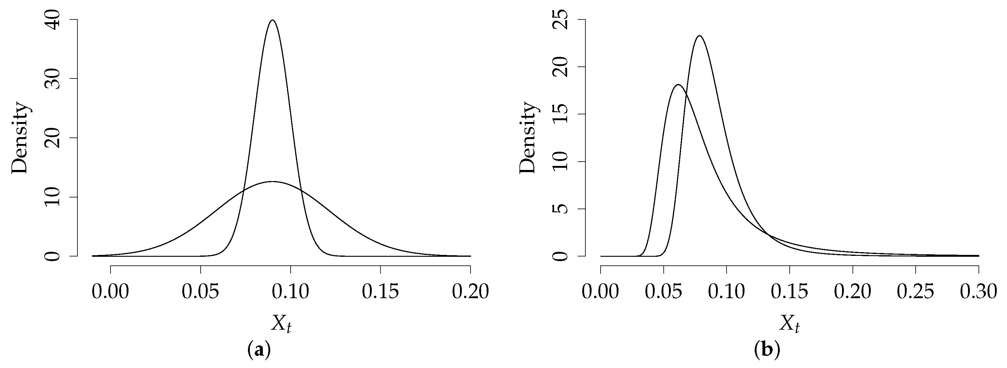
Table 1 shows the eight simulated scenarios for the Vasicek model, along with unconditional and conditional mean and variance, as the analytical density is available. The first two scenarios correspond to the low mean reversion, with increasing unconditional volatility, and the third and fourth are the high mean reversion cases. For the high persistent dependence scenarios (1 and 2) the parameter values are and , and for the low persistence (scenarios 3 and 4) the parameter are and . The marginal density was kept unchanged while varying the speed of mean reversion, therefore scenarios 1 and 3 and scenarios 2 and 4 have the same marginal density, as illustrated in Figure A1. The settings of scenarios 1 and 2 allow us to check the performance in a near unit-root case, as the regressive coefficient of is . Scenarios 5–8, although unrelated to real interest rate processes, are limiting cases to quantify the impact of persistence separately from changes in the marginal density. In scenarios 5 and 6 (7 and 8), the mean-reverting force is increased by a factor of 25 (49) from scenarios 1 and 2 and is changed in the same proportion to hold the marginal density fixed.
In regards to the scenarios for the CKLS model, a similar scheme was set, as shown in Table 1, keeping for all scenarios the same parameters for the drift function as the Vasicek. First two scenarios correspond to high persistent dependence with parameter values and , and for the low persistence (scenarios 3 and 4) the parameter are and . Figure A1 illustrates the stationary density for scenarios 1 and 2, where the parameter was increased by a factor of 4, just like from scenario 3 to 4.
Table 2 and Table 3 show the simulation study for the Vasicek model (along with Table A1, Table A2, Table A3, Table A4, deferred to Appendix A), Table 4 shows the computational performance of the methods, while Table 5 and Table 6 (and Table A5 and Table A6) refer to the CKLS model. The mean of the parameter estimates for the 1000 replications of the experiment is included, as well as standard deviation (SD) and root mean squared error (RMSE) for the estimation methods in Section 2:
- (i)
- Exact maximum likelihood (EML);
- (ii)
- Euler method (DML);
- (iii)
- Local linearization (LL);
- (iv)
- Hermite polynomial expansion (HP);
- (v)
- Generalized Method of Moments (GMM);
- (vi)
- Kalman Filter (KF);
- (vii)
- Markov Chain Monte Carlo (MCMC).
3.2. Implementation Details
The simulated sample paths for the Vasicek model were constructed from the closed-form transition density and for the CKLS model the Milstein scheme was used. To reduce discretization bias, paths were generated with daily frequency () and subsamples were taken on a weekly () or monthly () basis. The initial condition was set to be the average and the first 1000 data were discarded, as a burn-in period to remove the dependence on the initial value.
As in the CKLS model a closed form expression for the transition density is not available, the exact maximum likelihood method is not included, as it is unfeasible. The GMM was implemented with four moment conditions, where the first two identify the marginal distribution and the higher order are nonlinear functions of the first two moments. As the Vasicek model does have a closed form for the transition density, the true moments were used. Regarding the MCMC setup, for the Vasicek model the algorithm is iterated 2500 times and the first 500 iterations were discarded. The iterations were increased for the CKLS model as there is an additional parameter to sample, thus 5000 iterations were executed and the first 1000 were discarded. For both models, was fixed in the data augmentation step. For all methods, was jointly estimated. The drift parameter is calculated indirectly, as the drift specification was rewritten to estimate the intercept .
Regarding optimization, we chose to minimize the negative log-likelihood function and use the BFGS (Broyden–Fletcher–Goldfarb–Shanno) algorithm [24], where the gradient and Hessian matrix are calculated numerically in the optimization routine. As for the choice of initial values, the approach is the following: we fit a linear regression, writing the discrete version of the SDE as in Equation (13), to obtain a rough estimation of the parameters and set the starting values. For the CKLS diffusion parameter , we specified a power variance function for the heteroscedasticity structure.
Since some of the procedures are computationally expensive, we chose to integrate C and C++ code [43] in the R routines. Table 4 shows run-times for each Monte Carlo iteration, with sample size , and evidences the computational cost of simulation-based techniques, such as the MCMC. The Kalman filter benefits from using a lower-level programming language like C and has low run-times, though the remainder of the methods have a similar performance in base R, being the GMM the slowest.
3.3. Discussion
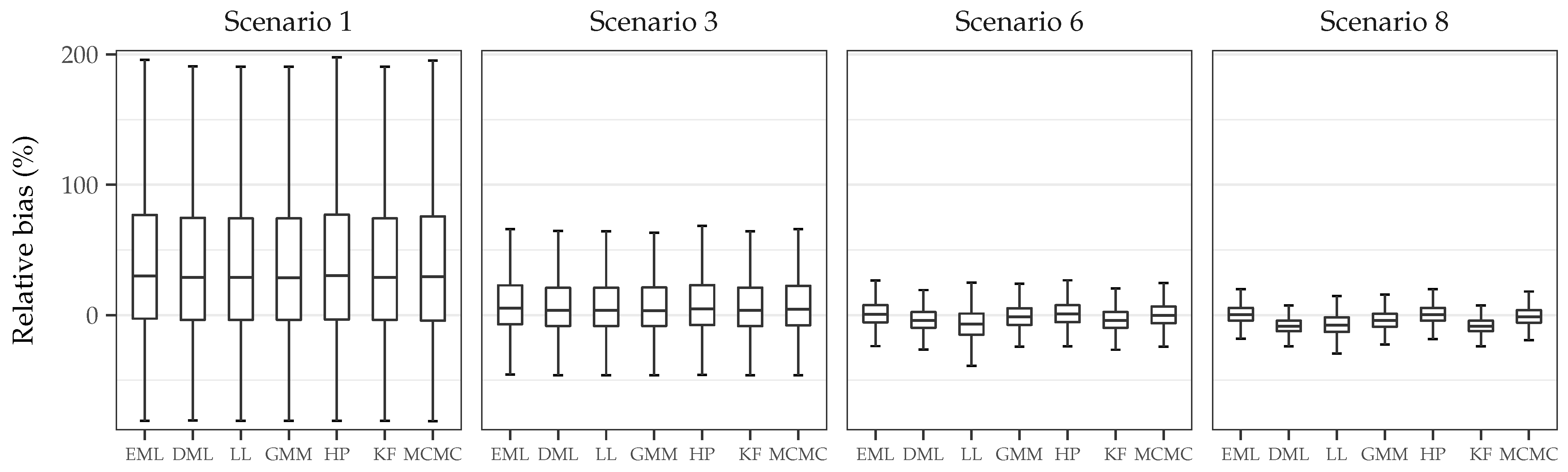
Table 2 and Table 5 report the estimates for scenario 1, for both Vasicek and CKLS models, which features low mean reversion and the unconditional volatility is very small, a quiet process whose estimation can be challenging. The process is nearly unit-root, which can increase the estimation bias in the drift parameter , as reported in [44]. This large bias in the estimation of the drift parameter , which controls the speed of mean reversion, is encountered in both tables with small sample size n through all estimation procedures, with more than a relative bias (see Figure 2). The RMSE in both models for is similar, the other parameters estimates have small RMSE but the parameters in the diffusion function incur in more bias in the CKLS model, as this model is relatively hard to identify as it may yield similar volatility functions for different values of and , while the Vasicek model has a simpler diffusion function. Both bias and RMSE decrease as n and the total observation time T are increased, especially for . As opposed to discrete time series, where the sample size n controls the estimation error, is T who defines the bias and variance of the estimations: the last two columns (weekly and monthly frequency) have similar observation time T but different sample size n, and RMSEs are close. Exact ML is available for the Vasicek model, thus avoiding discretization bias, but nevertheless biases are homogeneous for all methods, with GMM presenting a slightly higher RMSE.
When volatility is increased while keeping the same drift function (Table A1 and Table A5, in Appendix A), bias is moderately increased for and standard deviation is higher than in scenario 1 for the Vasicek model, while reducing for the diffusion parameters in the CKLS model, specially . All biases shrink as the sample size and observation time increases. The GMM method shows less efficiency, with a larger RMSE in the CKLS model.
The estimation bias of the drift parameter increases when the diffusion process has an absence of dynamics, which happens when is small. Scenarios 1 and 2 have a mean reversion parameter closer to zero, while scenarios 3 (Table 3 and Table 6) and 4 (Table A2 and Table A6) show high mean reversion. For the low volatility case, scenario 3, the finite sample bias of is significantly smaller (close to , see Figure 2) than the high persistence dependence scenarios for both models and estimation bias and standard deviation of is also reduced. For the CKLS model, the estimation bias of is reduced and the estimation error of is similar to scenario 1. RMSE and bias diminish with increasing n and T, with less RMSE in the weekly scenario for the CKLS model compared with the monthly simulation, which may be due to the discretization error. The higher volatility scenario shows a similar behavior, with smaller bias in the drift parameters than low mean reversion scenarios, but moderately higher in with respect to scenario 3, and the estimation errors for the diffusion parameters of the CKLS model are inferior compared to scenario 3.
Scenario 6 (Table A3) has a mean-reverting force five times higher than scenario 2 while keeping the same marginal distribution. In this setting, the estimation bias shrinks substantially in all schemes, as we are departing from the unit-root case. However, the discretization bias starts arising, as shown in the estimations of DML and KF methods with monthly frequency (note that scenario 5 is not included, as the results were very close and so too were the conclusions drawn) . This is magnified in the limiting case of scenario 8 (Table A4), where the estimation bias is very small in all schemes, but the discretization bias in DML, KF and, less so, in LL for and is large, mostly in the coarser discretization (monthly), noticeably underestimating both parameters (the performance of the methods was analogous in scenario 7, therefore results are not reported). Figure 3 illustrates true (black) and discretized (gray) log-likelihood for scenarios 1, 3, 6 and 8, where departures from the true log-likelihood are larger for lower mean reversion scenarios, while scenarios 6 and 8 display discretization bias.
The analysis of the Monte Carlo evidence reveals the following insights:
- (i)
- The dynamic of the process is governed by the drift parameter , which determines the persistence of the process by controlling the reversion towards the unconditional mean. As , mean reversion goes to zero and correlation between observations approaches one. This increases persistence, which introduces sample bias in parametric estimation [45]. Simulations show that increasing lowered persistence and, therefore, estimation bias was also diminished (see Figure 2). High persistence scenarios, near unit-root cases, revealed significant estimation bias in the drift parameter , but almost negligible in the diffusion parameter .
- (ii)
- Increasing the volatility parameters had minor effect on the estimators performance. In the Vasicek model, higher values in the volatility parameter slightly increased RMSE in the estimation of . On the other hand, the estimation of the parameters in the CKLS diffusion function benefit from richer volatility dynamics, reducing RMSE.
- (iii)
- In discrete time series, the bias and variance of estimators is controlled by the sample size n, so that they reduce as . In continuous-time models sampled at discrete time points, bias and variance in the estimation of the drift parameter is dominated by the total observation time . Under quite general conditions, the estimators of the drift parameters are of order , while the diffusion parameter is of order [46]. The simulated scenarios corroborate this, as estimation bias with and 43 years were close despite the different frequency (weekly and monthly, respectively) and sample size n (2600 and 520, respectively).
- (iv)
- Discretization bias arises in DML and KF methods in scenarios with low sampling frequency and low persistence (see Figure 3), and correcting the DML estimates with local linearization does not always correct the bias and both and are underestimated.
- (v)
- There appears to be similar estimation bias in the drift parameters for both Vasicek and CKLS models. However, the more flexible parametric form of the CKLS volatility function makes estimation more challenging, and bias and RMSE for those parameters are higher than for the Vasicek model.
- (vi)
- Regarding efficiency, as exact ML is available for the Vasicek model, it can be regarded as a benchmark. Overall, the estimations of the parameters are close to the EML performance, being the GMM the less efficient. The estimations differ when discretization bias arises.
Table 7 provides a summary of the properties and finite sample performance of the methods. Regarding accuracy, differences among the methods are not always clear and the context of application (e.g., the sampling interval) should be considered when choosing the estimation procedure. The HP shows the best trade-off between efficiency and speed—followed by the LL method—and MCMC exhibits good accuracy through all scenarios, however, the inherent time consuming implementation (methodologically and computationally) are major disadvantages. The performance of simpler discretization schemes, like the ones used in DML and KF, is conditioned on the sampling interval and should be avoided for large , otherwise, their efficiency is close to the other alternatives (see Figure 2). The generalized method of moments was outperformed in the majority of scenarios, notably with higher dimensions of the parameter vector .
4. Application to Euribor Series
In this section, we consider four data sets corresponding to four maturities (three, six, nine and twelve months) of the Euribor (Euro Interbank Offered Rate) interest rate series. This daily series expand from 15th October 2001 to 30th December 2005 (sample size of ), see Figure 4. Numerous models have been proposed to capture the dynamics of short-term interest rate, including those by [1,3,4,5,49]. As these models can be nested within the unrestricted model
proposed by [6], we will estimate the parameters with the methods presented in the previous section. We chose a different drift parametrization of the CKLS model in (18) to provide standard errors for all estimates, so none of them are estimated indirectly.
The results of the parameter estimation for the CKLS model are shown in Table 8, with the associated standard error in parentheses. The estimates obtained by the different approaches are considerable close, where the generalized method of moments seem to present the most noticeable disparity, mainly in the level effect parameter . This was already noticed in [50], where different values of where obtained using MLE and a GMM estimator. It is important to note that the standard error associated to the GMM estimation is larger than in the other approaches, which was already manifested in the simulations (see Table 5 and Table 6 and Table A5 and Table A6). Regarding the estimated values for the different maturities, for all time periods the series are persistent and the main variation comes from the parameters of the volatility function: increases with maturity and decreases. The parameter controls the relationship between the interest rate and the volatility, for all series we have which indicates that volatility tends to increase as the rate rises. The estimation in the Euribor 12 months for is close to 1, which would correspond to the diffusion process proposed by Brennan and Schwartz [49].
As goodness-of-fit test for diffusion processes are available in the literature, we will test the parametric form of the drift and diffusion functions estimated for the Euribor series. Table 9 shows the p-values for the goodness-of-fit test suggested by Monsalve-Cobis et al. [51]. The empirical p-value is significant for the drift function in every maturity. Conversely, the p-value for the volatility function leads to a strong rejection of the null hypothesis, implying that the model is inadequate to explain the volatility of the series, for every maturity.
To further analyze the fitted CKLS model, we will use a resampling procedure in the context of state space models (see Section 2.4) as it can provide insight into the validity of the model. The bootstrap technique developed in [52] is easily implemented with the innovations form of the Kalman filter and allows us to approximate the sampling distributions of the parameter estimates. Inference in state space models estimated using the Kalman filter is feasible because there exists an asymptotic theory, as seen in Section 2.4, under general conditions, the parameter estimates of a state space model are consistent and asymptotically normal. Focusing on the estimates for the Euribor 3 months, Table 10 shows the standard errors obtained from bootstrap resamples, along with the asymptotic standard errors and parameter estimates, and Figure 5 illustrates the bootstrap distribution (histogram) and the asymptotic Gaussian distribution (dashed line) of , with . Regarding the drift parameters ( and ), the bootstrap and asymptotic distributions are close, however, for the diffusion parameters ( and ), both distributions differ. This is consistent with the conclusions drawn from the goodness-of-fit test (see Table 9), where the parametric form of the drift was not rejected, but the diffusion function lead to a strong rejection. The bootstrap standard error of and is notable larger and the histograms show a slightly skewed distribution. This implies that the CKLS diffusion function specification is not able to explain the dynamics of the Euribor series, although the linear drift with mean reversion seems to be adequate. A deterministic parametric form of the diffusion function might be incapable of capturing the volatility behavior and a more intricate form, such as stochastic volatility, may be more suitable, which was already pointed out in the econometric literature, that find data are more accurately represented by a stochastic volatility model.
5. Conclusions
We reviewed parametric estimation methods for univariate time-homogeneous SDEs. Interest rate time series are highly persistent and this strong correlation through time challenges estimation, as its discretized counterpart corresponds to a near unit-root model. To address the problem of estimation and discretization bias, a comparative study of estimation methods was discussed under different settings. Based on the analysis of the simulation results, the following conclusions can be reached. First, estimation bias is large for the drift parameter , which controls the speed of mean-reversion, though smaller for the diffusion parameters. Lack of dynamics, that emerges when is small, increases this bias. Discretization bias was discerned in very low persistence scenarios with coarse discretization frequency. Second, the parameter of the diffusion function was accurately estimated in the Vasicek model, but the performance in the CKLS model was worse. Increasing the observation time T did reduce the bias, as expected, and increasing conditional volatility resulted in more accurate estimates. Third, estimation bias and variance is reduced as , rather than when only the sample size n is increased. This was illustrated in the simulations, where scenarios with different sample size n but similar T had comparable performances. Finally, regarding the parameter estimators, the GMM is the least efficient, while discrete maximum likelihood methods performed similarly, with LL and HP improving discretization bias over DML and KF. The MCMC method also provides efficient estimates; however, the more ad hoc implementation, highly model-dependent, makes its use more intricate than the other methods. All the procedures reviewed in this article are provided in the companion estsde R package.
Author Contributions
Conceptualization, M.F.-B., W.G.-M. and A.L.-P.; methodology, M.F.-B., W.G.-M. and A.L.-P.; software, A.L.-P.; formal analysis, A.L.-P.; investigation, A.L.-P.; writing—original draft preparation, A.L.-P.; writing—review and editing, M.F.-B., W.G.-M. and A.L.-P.; funding acquisition, M.F.-B. and W.G.-M. All authors have read and agreed to the published version of the manuscript.
Funding
The authors acknowledge support from grant MTM2016-76969-P from the Spanish Ministry of Economy and Competitiveness (cofunded with FEDER funds) and gratefully thank Spanish National Research Council for providing the computing resources of the Supercomputing Center of Galicia (CESGA).
Institutional Review Board Statement
Not applicable.
Informed Consent Statement
Not applicable.
Data Availability Statement
Not applicable.
Acknowledgments
The authors would like to thank two anonymous referees for their insightful suggestions and comments.
Conflicts of Interest
The authors declare no conflict of interest.
Appendix A
The appendix contains the tabulated results of the simulation study for the Vasicek and CKLS models. The Vasicek scenarios included here are 2, 4, 6 and 8 (see Table 1), which all of them have the same marginal distribution (see Figure A1), and scenarios 2 and 4 of the CKLS model.
Figure A1.
(a) Marginal density for Vasicek model, scenario 1 (3, 5 and 7) and 2 (4, 6 and 8) and (b) Marginal density for CKLS model, scenario 1 and 2.
Figure A1.
(a) Marginal density for Vasicek model, scenario 1 (3, 5 and 7) and 2 (4, 6 and 8) and (b) Marginal density for CKLS model, scenario 1 and 2.


Table A1.
Monte Carlo simulation for Vasicek model with . Boldfaces denote the best results in terms of bias, standard deviation and RMSE.
Table A1.
Monte Carlo simulation for Vasicek model with . Boldfaces denote the best results in terms of bias, standard deviation and RMSE.
| Scenario 2 | , | , | , | |||||||
|---|---|---|---|---|---|---|---|---|---|---|
| Method | Mean | SD | RMSE | Mean | SD | RMSE | Mean | SD | RMSE | |
| EML | ||||||||||
| DML | ||||||||||
| LL | ||||||||||
| HP | ||||||||||
| KF | ||||||||||
| MCMC | ||||||||||
| GMM | ||||||||||
Table A2.
Monte Carlo simulation for Vasicek model with .
| Scenario 4 | , | , | , | |||||||
|---|---|---|---|---|---|---|---|---|---|---|
| Method | Mean | SD | RMSE | Mean | SD | RMSE | Mean | SD | RMSE | |
| EML | ||||||||||
| DML | ||||||||||
| LL | ||||||||||
| HP | ||||||||||
| KF | ||||||||||
| Method | Mean | SD | RMSE | Mean | SD | RMSE | Mean | SD | RMSE | |
| MCMC | ||||||||||
| GMM | ||||||||||
Table A3.
Monte Carlo simulation for Vasicek model with .
| Scenario 6 | , | , | , | |||||||
|---|---|---|---|---|---|---|---|---|---|---|
| Method | Mean | SD | RMSE | Mean | SD | RMSE | Mean | SD | RMSE | |
| EML | ||||||||||
| DML | ||||||||||
| LL | ||||||||||
| HP | ||||||||||
| KF | ||||||||||
| MCMC | ||||||||||
| GMM | ||||||||||
Table A4.
Monte Carlo simulation for Vasicek model with .
| Scenario 8 | , | , | , | |||||||
|---|---|---|---|---|---|---|---|---|---|---|
| Method | Mean | SD | RMSE | Mean | SD | RMSE | Mean | SD | RMSE | |
| EML | ||||||||||
| DML | ||||||||||
| LL | ||||||||||
| HP | ||||||||||
| KF | ||||||||||
| MCMC | ||||||||||
| GMM | ||||||||||
Table A5.
Monte Carlo simulation for CKLS model with .
| Scenario 2 | , | , | , | |||||||
|---|---|---|---|---|---|---|---|---|---|---|
| Method | Mean | SD | RMSE | Mean | SD | RMSE | Mean | SD | RMSE | |
| DML | ||||||||||
| LL | ||||||||||
| HP | ||||||||||
| KF | ||||||||||
| Method | Mean | SD | RMSE | Mean | SD | RMSE | Mean | SD | RMSE | |
| MCMC | ||||||||||
| GMM | ||||||||||
Table A6.
Monte Carlo simulation for CKLS model with .
| Scenario 4 | , | , | , | |||||||
|---|---|---|---|---|---|---|---|---|---|---|
| Method | Mean | SD | RMSE | Mean | SD | RMSE | Mean | SD | RMSE | |
| DML | ||||||||||
| LL | ||||||||||
| HP | ||||||||||
| KF | ||||||||||
| MCMC | ||||||||||
| GMM | ||||||||||
References
- Merton, R.C. Theory of rational option pricing. Bell J. Econ. Manag. Sci. 1973, 4, 141–183. [Google Scholar] [CrossRef] [Green Version]
- Black, F.; Scholes, M. The pricing of options and corporate liabilities. J. Political Econ. 1973, 81, 637–654. [Google Scholar] [CrossRef] [Green Version]
- Vasicek, O. An equilibrium characterization of the term structure. J. Financ. Econ. 1977, 5, 177–188. [Google Scholar] [CrossRef]
- Brennan, M.J.; Schwartz, E.S. A continuous time approach to the pricing of bonds. J. Bank. Financ. 1979, 3, 133–155. [Google Scholar] [CrossRef]
- Cox, J.C.; Ingersoll, J.E., Jr.; Ross, S.A. An intertemporal general equilibrium model of asset prices. Econometrica 1985, 53, 363–384. [Google Scholar] [CrossRef] [Green Version]
- Chan, K.C.; Karolyi, G.A.; Longstaff, F.A.; Sanders, A.B. An empirical comparison of alternative models of the short-term interest rate. J. Financ. 1992, 47, 1209–1227. [Google Scholar] [CrossRef]
- Ahn, D.H.; Gao, B. A parametric nonlinear model of term structure dynamics. Rev. Financ. Stud. 1999, 12, 721–762. [Google Scholar] [CrossRef]
- Phillips, P.C.; Yu, J. Jackknifing bond option prices. Rev. Financ. Stud. 2005, 18, 707–742. [Google Scholar] [CrossRef] [Green Version]
- Stübinger, J.; Endres, S. Pairs trading with a mean–reverting jump–diffusion model on high–frequency data. Quant. Financ. 2018, 18, 1735–1751. [Google Scholar] [CrossRef] [Green Version]
- Endres, S.; Stübinger, J. Optimal trading strategies for Lévy-driven Ornstein–Uhlenbeck processes. Appl. Econ. 2019, 51, 3153–3169. [Google Scholar] [CrossRef]
- Amorino, C.; Gloter, A. Contrast function estimation for the drift parameter of ergodic jump diffusion process. Scand. J. Stat. 2020, 47, 279–346. [Google Scholar] [CrossRef] [Green Version]
- Endres, S.; Stübinger, J. A flexible regime switching model with pairs trading application to the S&P 500 high–frequency stock returns. Quant. Financ. 2019, 19, 1727–1740. [Google Scholar] [CrossRef] [Green Version]
- Sørensen, H. Parametric inference for diffusion processes observed at discrete points in time: A survey. Int. Stat. Rev. 2004, 72, 337–354. [Google Scholar] [CrossRef] [Green Version]
- Hurn, A.S.; Jeisman, J.; Lindsay, K.A. Seeing the wood for the trees: A critical evaluation of methods to estimate the parameters of stochastic differential equations. J. Financ. Econom. 2007, 5, 390–455. [Google Scholar] [CrossRef] [Green Version]
- Shoji, I.; Ozaki, T. Comparative study of estimation methods for continuous time stochastic processes. J. Time Ser. Anal. 1997, 18, 485–506. [Google Scholar] [CrossRef]
- Durham, G.B.; Gallant, A.R. Numerical techniques for maximum likelihood estimation of continuous-time diffusion processes. J. Bus. Econ. Stat. 2002, 20, 297–338. [Google Scholar] [CrossRef] [Green Version]
- Ozaki, T. A bridge between nonlinear time series models and nonlinear stochastic dynamical systems: A local linearization approach. Stat. Sin. 1992, 2, 113–135. [Google Scholar]
- Shoji, I.; Ozaki, T. Estimation for nonlinear stochastic differential equations by a local linearization method. Stoch. Anal. Appl. 1998, 16, 733–752. [Google Scholar] [CrossRef]
- Aït-Sahalia, Y. Maximum Likelihood Estimation of Discretely Sampled Diffusions: A Closed-form Approximation Approach. Econometrica 2002, 70, 223–262. [Google Scholar] [CrossRef]
- Kalman, R.E. A new approach to linear filtering and prediction problems. J. Basic Eng. 1960, 82, 35–45. [Google Scholar] [CrossRef] [Green Version]
- Elerian, O.; Chib, S.; Shephard, N. Likelihood inference for discretely observed nonlinear diffusions. Econometrica 2001, 69, 959–993. [Google Scholar] [CrossRef]
- Eraker, B. MCMC analysis of diffusion models with application to finance. J. Bus. Econ. Stat. 2001, 19, 177–191. [Google Scholar] [CrossRef]
- Hansen, L.P. Large sample properties of generalized method of moments estimators. Econometrica 1982, 1029–1054. [Google Scholar] [CrossRef]
- R Core Team. R: A Language and Environment for Statistical Computing; R Foundation for Statistical Computing: Vienna, Austria, 2014. [Google Scholar]
- Karatzas, I.; Shreve, S. Brownian Motion and Stochastic Calculus; Springer: Berlin/Heidelberg, Germany, 1998; Volume 113. [Google Scholar] [CrossRef]
- Maruyama, G. Continuous Markov processes and stochastic equations. Rend. Circ. Mat. Palermo 1955, 4, 48. [Google Scholar] [CrossRef]
- Kloeden, P.E.; Platen, E. Numerical Solution of Stochastic Differential Equations; Springer: Berlin/Heidelberg, Germany, 1992. [Google Scholar] [CrossRef] [Green Version]
- Elerian, O. A Note on the Existence of a Closed Form Conditional Transition Density for the Milstein Scheme; Working Paper; Nuffield College, Oxford University: Oxford, UK, 1998. [Google Scholar]
- Florens-Zmirou, D. Approximate discrete-time schemes for statistics of diffusion processes. Statistics 1989, 20, 547–557. [Google Scholar] [CrossRef]
- Caines, P.E. Linear Stochastic Systems; Wiley: New York, NY, USA, 1988. [Google Scholar]
- Dempster, A.P.; Laird, N.M.; Rubin, D.B. Maximum likelihood from incomplete data via the EM algorithm. J. R. Stat. Soc. Ser. B Stat. Methodol. 1977, 39, 1–22. [Google Scholar] [CrossRef]
- Shumway, R.H.; Stoffer, D.S. An approach to time series smoothing and forecasting using the EM algorithm. J. Time Ser. Anal. 1982, 3, 253–264. [Google Scholar] [CrossRef]
- Jones, R.H. Maximum likelihood fitting of ARMA models to time series with missing observations. Technometrics 1980, 22, 389–395. [Google Scholar] [CrossRef]
- Pagan, A. Some identification and estimation results for regression models with stochastically varying coefficients. J. Econom. 1980, 13, 341–363. [Google Scholar] [CrossRef]
- Ljung, L.; Caines, P.E. Asymptotic normality of prediction error estimators for approximate system models. Stochastics 1980, 3, 29–46. [Google Scholar] [CrossRef]
- Hannan, E.J.; Deistler, M. The Statistical Theory of Linear Systems; Wiley: New York, NY, USA, 1988. [Google Scholar] [CrossRef]
- Harvey, A.C. Forecasting, Structural Time Series Models and the Kalman Filter; Cambridge University Press: Cambridge, UK, 1990. [Google Scholar] [CrossRef]
- Jazwinski, A.H. Stochastic Processes and Filtering Theory; Academic Press: New York, NY, USA, 1970. [Google Scholar]
- Singer, H. Parameter estimation of nonlinear stochastic differential equations: Simulated maximum likelihood versus extended Kalman filter and Itô-Taylor expansion. J. Comput. Graph. Stat. 2002, 11, 972–995. [Google Scholar] [CrossRef]
- Kloeden, P.E.; Platen, E. Higher-order implicit strong numerical schemes for stochastic differential equations. J. Stat. Phys. 1992, 66, 283–314. [Google Scholar] [CrossRef]
- Newey, W.K.; McFadden, D. Large sample estimation and hypothesis testing. Handb. Econom. 1994, 4, 2111–2245. [Google Scholar]
- Uhlenbeck, G.E.; Ornstein, L.S. On the theory of the Brownian motion. Phys. Rev. 1930, 36, 823. [Google Scholar] [CrossRef]
- Eddelbuettel, D.; François, R. Rcpp: Seamless R and C++ Integration. J. Stat. Softw. 2011, 40, 1–18. [Google Scholar] [CrossRef] [Green Version]
- Yu, J.; Phillips, P.C. A Gaussian approach for continuous time models of the short-term interest rate. Econom. J. 2001, 4, 210–224. [Google Scholar] [CrossRef]
- Ball, C.A.; Torous, W.N. Unit roots and the estimation of interest rate dynamics. J. Empir. Financ. 1996, 3, 215–238. [Google Scholar] [CrossRef] [Green Version]
- Tang, C.Y.; Chen, S.X. Parameter estimation and bias correction for diffusion processes. J. Econom. 2009, 149, 65–81. [Google Scholar] [CrossRef] [Green Version]
- Aït-Sahalia, Y. Transition densities for interest rate and other nonlinear diffusions. J. Financ. 1999, 54, 1361–1395. [Google Scholar] [CrossRef]
- Kalman, R.E. Mathematical description of linear dynamical systems. J. Soc. Ind. Appl. Ser. A Control 1963, 1, 152–192. [Google Scholar] [CrossRef]
- Brennan, M.J.; Schwartz, E.S. Analyzing convertible bonds. J. Financ. Quant. 1980, 15, 907–929. [Google Scholar] [CrossRef]
- Pagan, A.R.; Hall, A.D.; Martin, V. Modeling the term structure. Handb. Stat. 1996, 14, 91–118. [Google Scholar] [CrossRef]
- Monsalve-Cobis, A.; González-Manteiga, W.; Febrero-Bande, M. Goodness-of-fit test for interest rate models: An approach based on empirical processes. Comput. Stat. Data Anal. 2011, 55, 3073–3092. [Google Scholar] [CrossRef]
- Stoffer, D.S.; Wall, K.D. Bootstrapping state-space models: Gaussian maximum likelihood estimation and the Kalman filter. J. Am. Stat. Assoc. 1991, 86, 1024–1033. [Google Scholar] [CrossRef]
Figure 1.
Augmented data in the discretization scheme: the observed data, and , is augmented by introducing unobserved data points.
Figure 1.
Augmented data in the discretization scheme: the observed data, and , is augmented by introducing unobserved data points.
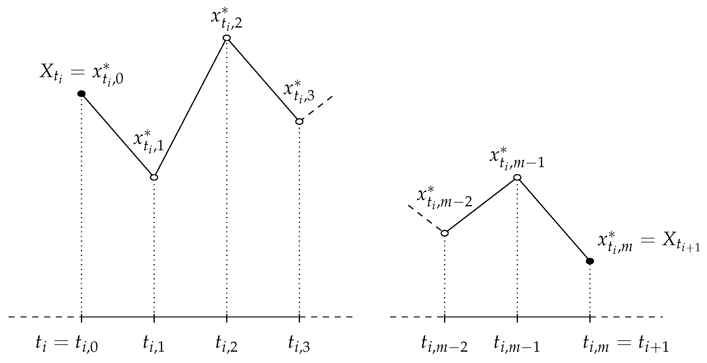
Figure 2.
Relative bias (in percentage) for the drift parameter with weekly data () and .

Figure 3.
Vasicek model log-likelihood (ℓ) for the drift parameter with known () and estimated () parameters, where is the true value. The true density and its discretized version () is illustrated, along with the estimate obtained ( and , respectively). Note that scenarios with same but different volatility parameter (scenarios 2, 4, 5 and 7, respectively) are not included, as the estimates were very close and figures very similar to the ones displayed.

Figure 4.
Euribor series. Daily evolution for the time period between 15th October 2001 and 30th December 2005. Sample size for each data set is . From left to right, Euribor 3, 6, 9 and 12 months, respectively.
Figure 4.
Euribor series. Daily evolution for the time period between 15th October 2001 and 30th December 2005. Sample size for each data set is . From left to right, Euribor 3, 6, 9 and 12 months, respectively.

Figure 5.
Bootstrap histogram of , with , and asymptotic Gaussian distribution for the CKLS model, , fitted to Euribor 3 months series.
Figure 5.
Bootstrap histogram of , with , and asymptotic Gaussian distribution for the CKLS model, , fitted to Euribor 3 months series.
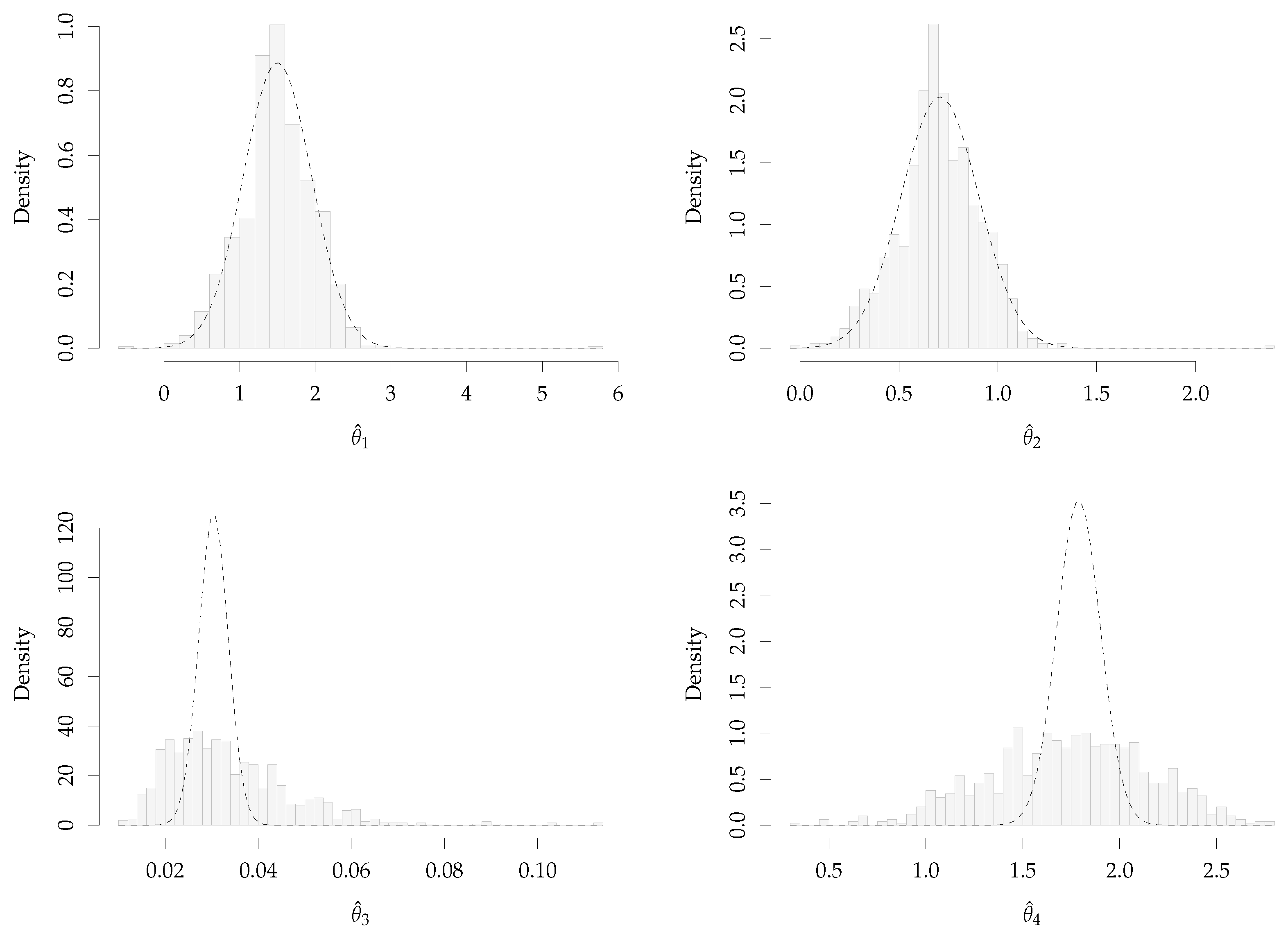
Table 1.
Scenarios for the Monte Carlo study for the Vasicek, , and CKLS, , models with .
| Vasicek | Scenario 1 | Scenario 2 | Scenario 3 | Scenario 4 |
|---|---|---|---|---|
| Vasicek | Scenario 5 | Scenario 6 | Scenario 7 | Scenario 8 |
| CKLS | Scenario 1 | Scenario 2 | Scenario 3 | Scenario 4 |
Table 2.
Monte Carlo simulation for Vasicek model, , scenario 1: low mean reversion and low volatility. Boldfaces denote the best results in terms of bias, standard deviation and RMSE.
Table 2.
Monte Carlo simulation for Vasicek model, , scenario 1: low mean reversion and low volatility. Boldfaces denote the best results in terms of bias, standard deviation and RMSE.
| Scenario 1 | , | , | , | |||||||
|---|---|---|---|---|---|---|---|---|---|---|
| Method | Mean | SD | RMSE | Mean | SD | RMSE | Mean | SD | RMSE | |
| EML | ||||||||||
| DML | ||||||||||
| LL | ||||||||||
| HP | ||||||||||
| KF | ||||||||||
| MCMC | ||||||||||
| GMM | ||||||||||
Table 3.
Monte Carlo simulation for Vasicek model, , scenario 3: high mean reversion and low volatility. Boldfaces denote the best results in terms of bias, standard deviation and RMSE.
Table 3.
Monte Carlo simulation for Vasicek model, , scenario 3: high mean reversion and low volatility. Boldfaces denote the best results in terms of bias, standard deviation and RMSE.
| Scenario 3 | , | , | , | |||||||
|---|---|---|---|---|---|---|---|---|---|---|
| Method | Mean | SD | RMSE | Mean | SD | RMSE | Mean | SD | RMSE | |
| EML | ||||||||||
| DML | ||||||||||
| LL | ||||||||||
| HP | ||||||||||
| KF | ||||||||||
| MCMC | ||||||||||
| GMM | ||||||||||
Table 4.
CPU time (in seconds) of the estimation methods per iteration, with .
| Time (Seconds) | EML | DML | LL | HP | KF | MCMC | GMM |
|---|---|---|---|---|---|---|---|
| Vasicek | 0.0534 | 0.0469 | 0.0424 | 0.4921 | 0.1097 | 50.8442 | 1.0108 |
| CKLS | - | 0.0818 | 0.2011 | 1.9543 | 0.2017 | 140.5385 | 2.0237 |
| Implementation: | R | R | R | R | C | C++ | R/C++ |
Table 5.
Monte Carlo simulation for CKLS model, , scenario 1: low mean reversion and low volatility. Boldfaces denote the best results in terms of bias, standard deviation and RMSE.
Table 5.
Monte Carlo simulation for CKLS model, , scenario 1: low mean reversion and low volatility. Boldfaces denote the best results in terms of bias, standard deviation and RMSE.
| Scenario 1 | , | , | , | |||||||
|---|---|---|---|---|---|---|---|---|---|---|
| Method | Mean | SD | RMSE | Mean | SD | RMSE | Mean | SD | RMSE | |
| DML | ||||||||||
| LL | ||||||||||
| HP | ||||||||||
| KF | ||||||||||
| MCMC | ||||||||||
| GMM | ||||||||||
Table 6.
Monte Carlo simulation for CKLS model, , scenario 3: high mean reversion and low volatility. Boldfaces denote the best results in terms of bias, standard deviation and RMSE.
Table 6.
Monte Carlo simulation for CKLS model, , scenario 3: high mean reversion and low volatility. Boldfaces denote the best results in terms of bias, standard deviation and RMSE.
| Scenario 3 | , | , | , | |||||||
|---|---|---|---|---|---|---|---|---|---|---|
| Method | Mean | SD | RMSE | Mean | SD | RMSE | Mean | SD | RMSE | |
| DML | ||||||||||
| LL | ||||||||||
| HP | ||||||||||
| KF | ||||||||||
| MCMC | ||||||||||
| GMM | ||||||||||
Table 7.
Summary of estimation procedures for SDE parameters.
| Method | Authors | Asymptotic Properties | Finite Sample Performance |
|---|---|---|---|
| DML | Florens–Zmirou [29] | Asymptotically normal and consistent | Biased when is large |
| LL | Ozaki [17] Shoji and Ozaki [18] | As ML estimators | Outperforms discrete ML and KF |
| HP | Aït–Sahalia [19,47] | Asymptotically normal and consistent [19] | Outperforms LL |
| KF | Kalman [20,48] | Asymptotically normal and consistent [30,34] | Similar to discrete ML |
| MCMC | Elerian et al. [21] Eraker [22] | Simulation based | Efficient but the most computationally intensive |
| GMM | Hansen [23] Chan et al. [6] | Asymptotically normal and consistent [23,41] | The least efficient and efficiency depends on moments |
Table 8.
Estimated parameters and standard errors (in parentheses) for the CKLS model, , fitted to Euribor series using six estimation methods.
Table 8.
Estimated parameters and standard errors (in parentheses) for the CKLS model, , fitted to Euribor series using six estimation methods.
| Method | 3 Months | 6 Months | 9 Months | 12 Months | |||||
|---|---|---|---|---|---|---|---|---|---|
| DML | |||||||||
| LL | |||||||||
| HP | |||||||||
| KF | |||||||||
| MCMC | |||||||||
| GMM | |||||||||
Table 9.
p-values for the Monsalve-Cobis et al. [51] goodness-of-fit test for the CKLS parametric form of the drift and diffusion functions.
Table 9.
p-values for the Monsalve-Cobis et al. [51] goodness-of-fit test for the CKLS parametric form of the drift and diffusion functions.
| Maturity: | 3 Months | 6 Months | 9 Months | 12 Months |
|---|---|---|---|---|
| p-value drift function | ||||
| p-value volatility function | <0.001 | <0.001 |
Table 10.
Kalman filter estimates, asymptotic standard error and bootstrap standard error of the CKLS model fitted to Euribor 3 months serie.
Table 10.
Kalman filter estimates, asymptotic standard error and bootstrap standard error of the CKLS model fitted to Euribor 3 months serie.
| Parameters: | ||||
|---|---|---|---|---|
| Estimation | 1.4964 | 0.7049 | 0.0303 | 1.7899 |
| Asymptotic standard error | 0.4492 | 0.1964 | 0.0031 | 0.1121 |
| Bootstrap standard error | 0.4794 | 0.2105 | 0.0653 | 0.4110 |
Publisher’s Note: MDPI stays neutral with regard to jurisdictional claims in published maps and institutional affiliations. |
© 2021 by the authors. Licensee MDPI, Basel, Switzerland. This article is an open access article distributed under the terms and conditions of the Creative Commons Attribution (CC BY) license (https://creativecommons.org/licenses/by/4.0/).
Share and Cite
MDPI and ACS Style
López-Pérez, A.; Febrero-Bande, M.; González-Manteiga, W. Parametric Estimation of Diffusion Processes: A Review and Comparative Study. Mathematics 2021, 9, 859. https://doi.org/10.3390/math9080859
AMA Style
López-Pérez A, Febrero-Bande M, González-Manteiga W. Parametric Estimation of Diffusion Processes: A Review and Comparative Study. Mathematics. 2021; 9(8):859. https://doi.org/10.3390/math9080859
Chicago/Turabian StyleLópez-Pérez, Alejandra, Manuel Febrero-Bande, and Wencesalo González-Manteiga. 2021. "Parametric Estimation of Diffusion Processes: A Review and Comparative Study" Mathematics 9, no. 8: 859. https://doi.org/10.3390/math9080859
Note that from the first issue of 2016, this journal uses article numbers instead of page numbers. See further details here.