
Chemical Identification from Raman Peak Classification Using Fuzzy Logic and Monte Carlo Simulation


Diagnostic and Metrology Laboratory, Department of Fusion and Technology for Nuclear Safety and Security, ENEA via Enrico Fermi 45, 00044 Frascati, Italy
*
Author to whom correspondence should be addressed.
Chemosensors 2022, 10(8), 295; https://doi.org/10.3390/chemosensors10080295
Submission received: 23 June 2022
/
Revised: 21 July 2022
/
Accepted: 25 July 2022
/
Published: 27 July 2022
(This article belongs to the Special Issue Optical Chemical Sensors and Spectroscopy)
Abstract
:In spite of the wide use of Raman spectroscopy for chemical analysis in different fields, not any automated identification of Raman spectra is universally adopted. However, the interest in this field is witnessed by the large number of papers published in the last decades. The problem of Raman-spectra classification becomes particularly challenging when low irradiation is requested, either for safety reasons or to avoid target photodegradation. This often leads to spectra characterized by a low signal-to-noise ratio, where methods based on correlation usually fail. For this reason, a method based on peak identification through FMFs is presented, discussed and validated over a large set of samples. In particular, a Monte Carlo simulation has been employed to determine the best parameters of the fuzzy membership functions based on the analysis of performances of the classification procedure. The ROC curves have been analyzed, and AUC and best accuracy are employed as key parameters to evaluate the classification performances on different amounts of ammonium nitrate (from 300 to 1500 g) and different laser exposure levels (from 3.1 to 250 mJ/cm).
1. Introduction
The problem of automatic identification of substances using spectroscopic data (or other variables related to their structure as shape or composition) arose when automated data collection and processing became available. In general, the problem of automatic detection of patterns within a dataset may assume several aspects, according to the nature of the being under examination (elements, chemical bonds, functional groups, cells, bacteria, yeasts, algae, but also faces, handwriting, objects and shapes in pictures). Nevertheless, some common characteristics can be found in all these problems, and they have become, in the last decades, the object of a specific field of information theory named pattern recognition. On the other hand, the real-time possibility of detecting specific materials on complex surfaces assumes great importance in many cases. Security, geology (both terrestrial and planetary), biology and medicine, environmental and cultural heritage monitoring are some fields where Raman spectroscopy is largely used for real-time analyses [1,2,3,4,5], where the need for rapid answers on mixed samples is particularly felt. For example, the task of detecting traces of dangerous materials on clothes, luggage or sampling filters or identifying the pigments used in a mixed and overlaid paint requires high sensitivity, specificity and, possibly low operating costs. Moreover, all these cases require the rapid detection of compounds and analysis of complex targets without sample preparation.
Raman spectroscopy is used in these fields thanks to its high specificity, sensitivity and low operating cost. Depending on the specific setup employed, no sample preparation is needed and may be also compliant with laser exposure regulations on people [6]. On the other hand, Raman spectroscopy needs the detection of low level signals, since in general, the Raman cross-section is smaller than the elastic one by several orders of magnitude. This is particularly true for traditional Raman spectroscopy, where no resonance lines nor surface enhancement can be exploited; though this is certainly a drawback of this technique for standoff detection or, in general, when a sample cannot be prepared (e.g., ancient paintings or frescoes), this approach remains the only option. In addition, sometimes, a low laser exposure is required to avoid damaging the sample or for safety regulations, according to IEC 60825-1 and European regulations [7].
The retrieval of sample composition by automated spectrum analysis must then be robust and reliable also in case of low signal-to-noise (SNR) ratios. For this reason, a long history of automated detection has been developed in the last few decades. In fact, the automatic identification of species from specific spectral information is a field that dates back to the 1960s, when computers started allowing automatic data collection and analysis, and they were focused on the recognition of peaks in a scintillation spectrum [8]. The attention on this subject suddenly rose, and the first reviews appeared in the early 1980s [9].
Since then, more sophisticated analyses have been attempted, using multivariate analysis [10], pattern recognition techniques [11,12], neural networks [13,14,15] and Linear Predictive Coding [16]. As observed in [17], multivariate analysis typically has some disadvantages, from the variations in the spectral background to the need of a fine calibration of the spectra. For these reasons, alternative approaches that employ relevant regions of the spectra have been developed. More recently, even organism classification by cytometric and/or micro-Raman data has been attempted [18,19,20,21,22]. Such problems, under a mathematical point of view, are related to tree classification from a hyperspectral fingerprint [23,24,25,26,27].
Again, the same problem was discussed in [28]. In this paper, the authors described an automated algorithm for the detection of explosives using UV Raman scattering. The spectra recorded by the system were processed to remove the fluorescence spectrum of the substrate using a Kaiser filter in the frequency domain. This allowed filtering out both low frequencies caused by fluorescence and high frequencies due to noise. The classification is committed to an inner product between the filtered spectrum and the reference ones. Such a procedure allowed a very good performance in detecting tri-nitro-toluene (TNT) and ammonium nitrate (AN) down to concentrations of 55 and 27 mg/cm, respectively. However, some false positives were detected as well, although a study of the Receiving Operating Curves (ROC) helps in minimizing the false alarm ratio while keeping a high true positive detection. However, this approach is not very promising for noisy signals, as discussed in the following sections. Other recent approaches involve deep neural networks, machine learning [29], and deep learning [30].
Fuzzy logic has been applied to Raman spectroscopy since 2002 [31]. To enhance the Raman signal, the authors designed and tested a filter based on fuzzy membership functions and fuzzy rules to filter out both shot noise and cosmic rays. In the following [32], fuzzy logic was applied to the out-and-out spectral identification, using a parabolic fit of overlapping sets in the spectrum. If a number of contiguous sets shows ‘similar’ negative quadratic coefficients, the peak is considered as a Raman band, trusting that noise-induced coefficients are independent and vary from one fit to the next. In a subsequent work [33], fuzzy logic was applied to the identification of species through the similarity between whole spectra, which is measured by the application of fuzzy rules to the correlation coefficients among the detected spectrum and the reference ones. However, the correlation coefficient is not a robust marker of closeness, especially for noisy or overlapped spectra, so this fuzzy approach was applied in synergy with principal component analysis [34], and since then, it has been used in combination with multivariate analysis [35] and genetic algorithms [36].
To avoid uncertainties tied to the low reliability of the correlation coefficient, fuzzy logic was also employed taking into account the positions of the detected peaks and comparing them with a reference database through suitable fuzzy rules [37]. The use of fuzzy membership functions allowed avoiding sharp thresholds to decide whether bands are close enough to be compatible or not. However, the rules employed took into account only the positions of the peaks and, what is more, they were applied to high SNR signals. In fact, the authors remind that for good performances, “it is required that the experimental conditions of measurement should be as suitable as possible”. In this paper, we will focus on the problem of the automatic recognition of species through the analysis of their Raman spectra using fuzzy rules coupled to a Monte Carlo simulation to optimize the parameters of the fuzzy membership functions. The algorithm, as well as the experimental conditions, are presented in Section 2, while the discussion and results are reported in Section 3.
2. Materials and Methods
2.1. Algorithm and Performance Evaluation
We can describe the problem of spectral identification in the following way: we need to recognize some specific features (fingerprint) within a structure, mostly a one-dimension vector (spectrum). Many types of spectra show narrow peaks, which are related to peculiar emission or absorption of the material under study (Raman, IR, atomic emission, mass spectrometry,…), while others, such as fluorescence, are in general observed as broad bands often overlapping each other. We will refer now to the first kind of spectra, where the fingerprint is constituted by the position and the amplitude of the observed peaks. Usually, the algorithms for spectral identification operate in two consecutive steps: first, data are pre-processed in order to transform the original input variable space into a new one, where the problem of pattern recognition and classification is easier to solve. This aspect of the pattern recognition is hence related to the problem of variable reduction and data mining. However, particular attention must be paid in order not to lose too much information in such a transformation. This key step requires an accurate selection of the transformation, both for computational speed and for an easier separation of output variables. The physics behind the specific problem may help to select the variables in the most efficient way. For example, it can be possible to discard those zones where the input variable does not carry effective information (these regions are typically called background: for example, in a spectrum, it is a range without peaks). The second step of the pattern recognition is the actual ‘recognition’ of each subject under investigation by comparison with a reference database. If the reference vectors are known and finite, a classification of the input data into the output categories is possible. The ‘closeness’ between two spectra is usually evaluated by means of a metric in the variable space such as the Euclidean distance or the correlation between the two vectors or subvectors. However, many issues are tied to this approach: first, the presence of more peaks in case of mixed compounds may alter the distance or the correlation even in sub-regions of the spectra. Second, the noise contributes to lower the correlation or raise the distance between two similar spectra. Figure 1 (right) shows an ideal spectrum S1 (orange) together with the same spectrum added to Gaussian noise S2 (blue). The SNR of this spectrum is calculated as the maximum of the weakest peak divided by the standard deviation of the signal in a zone without peaks. As the variance of the noise increases, the SNR decreases. The correlation coefficient r and the normalized Euclidean distance D can be calculated as:
and
where S1 represents the reference signal and S2 represents the test signal. These quantities are shown versus the SNR of the spectrum in the right panel: neither of them can be useful for an efficient identification of the noisier spectra. The question is: how low can the SNR be for a reasonable detection? Is there a method that performs better?
For this reason, in this work, we adopted a different approach. Since noise may also alter the form and the position of the maximum of peaks, a fuzzy logic approach may help overcome some issues caused by noise and enhance the identification performances for weak signals. The algorithm presented here has been developed first for the RAman Detection of Explosives instrument (RADEX) within the framework of the Standex (STANd-off Detection of Explosives) project [38] and refined since then. The development of automated recognition algorithms from Raman spectra started from the identification of the following critical points:
- 1.
- The effects of low SNR on the fingerprint important features (height, width and position of peaks). As stated before, in many cases, we expect the spectra to be noisy (i.e., single-shot spectroscopy and/or trace detection), in particular when eye-safe conditions or when low fluence is requested for preservation of the sample. This causes weaker peaks to be masked by noise, and it makes the exact position of the maximum to be not completely reliable also for detectable peaks.
- 2.
- Simultaneous strong contribution of fluorescence that can mask the weak Raman signal. In fact, to enhance the Raman cross-section, the wavelength employed often falls in the UV region, where the substrate or the compound itself may generate a fluorescence signal, which is often orders of magnitude higher than the Raman signal. Although it may happen that a strong fluorescence hides the Raman signal and make any detection impossible (because of the channel-to-channel variability due to the shot noise), it is often possible to filter out the contribution of fluorescence using band-pass filters over the acquired signal. However, a thorough discussion of this topic cannot be addressed here. In-depth analyses can be found in [39,40].
- 3.
- Possibility of overlaid spectra that can interfere with the algorithm. For many samples, an overlay of more reference (or even unknown) spectra can be expected (i.e., identification of pigments in paints or frescoes, mixtures of molecules in pharmacology). In all these cases, multivariate analysis of the signal is not expected to lead to good results, since most of the spectrum cannot be reliably correlated to the reference spectra unless specific subranges are selected.
The approach used by the authors established hence to avoid both the Euclidean distance between the spectra (intended as the sum of the squared differences between correspondent channels) and the correlation between them (intended as the inner product) because of the strong interference of the many bins carrying only noise or because of the peaks belonging to other Raman active molecules. Moreover, a strong fluorescence can be detected together with the Raman spectra because of substrate or ligands or the molecule itself, and in this case, linear correlation and Euclidean distance become totally misleading unless an effective pre-processing is performed to filter very efficiently low-frequency trends in the spectrum. Then, the idea is to exploit directly some important parameters associated to the peaks. This reduces the vector dimension (a few parameters for each peak are retrieved) and eliminates the influence of the baseline and the background noise, provided that peaks can be identified. More precisely, from the reference spectrum, the position, amplitude and width of selected peaks are retrieved, so that for each peak, three parameters are stored. The developed algorithm is then articulated in two steps:
2.2. Recognition of Peaks
This process involves a pre-processing of the data in order to prepare the dataset in the most efficient way for the recognition (i.e., filtering, transforming, mapping) and extracting a few parameters that refer to each detected peak (i.e., position, width, amplitude).
Although this step is often directly performed over the whole spectrum, through the minimization of a kind of distance in a suitable space between the spectrum under recognition and a reference database (in case after the pre-processing), we decided to exploit the parameters extracted after a fitting procedure over the regions where peaks are expected.
More in detail, a Lorentzian curve with four free parameters has been assumed as a fitting curve of each peak. The equation employed is of the form:
where a represents the offset, b represents the amplitude of the peak, c represents the modal value and d represents the width. The main advantage of the Lorentzian curve is that it is an algebraic curve, allowing faster calculation with respect to a Gaussian. The slowest convergence to zero of the tails did not represent an issue when fitting noisy peaks. Since the nonlinear fitting procedures critically depend on the initial guess of the parameters, automated initialization was performed on a subset around the peak of interest. The following choice of initial parameters was made if X and Y are the bin and the signal values:
where X|max(Y) gives the X value corresponding to the maximum value of Y and X|90prct(Y) give the X value corresponding to the 90th percentile of the Y values within the considered fitting subrange. The best value of the percentile depends on the width of the peak with respect to the resolution of the sampled spectrum; in our data, the 90th percentile performed well, and all fits converged to finite values. An example is shown in Figure 2.
The offset a depends on the background illumination, dark noise and other uninteresting properties of the spectrum, and it is not considered for the analysis. Therefore, for each peak, the three parameters b, c and d provide all the information needed for the identification.
2.3. Identification of Species
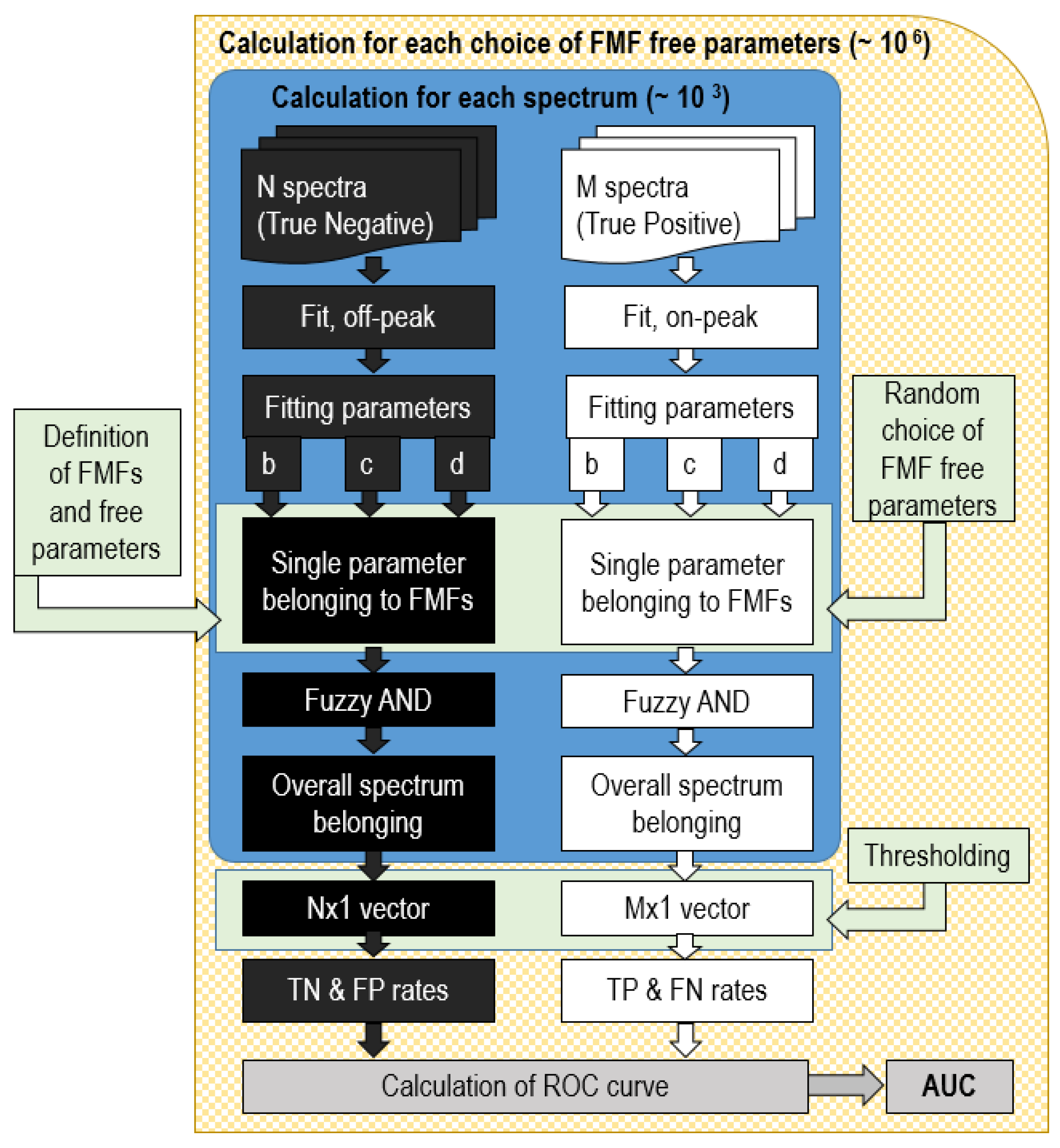
In order to classify the peak, these parameters can be compared to the same parameters determined from the sample spectrum. The idea is that the parameter distributions over a large number of spectra are sufficiently different in regions where no peaks are present from those obtained in the presence of a peak. Moreover, the strength of considering all the parameters at the same time relies on the fact that the off-peak fit parameter distributions are likely uncorrelated, so even if one value matches to a reference, the others will probably fall outside the acceptable interval. Nevertheless, for a binary classifier based on many sharp thresholds (i.e., less than, greater than), it may be not straightforward to evaluate the performances in terms of sensitivity and specificity. To avoid these problems, fuzzy membership functions (FMFs) were adopted for each parameter so that each parameter obtains a degree of belonging to the corresponding set. In fuzzy logic, the smooth boundary of fuzzy sets leads to a continuous belonging degrees (from 0 to 1), so all intermediate values are possible. In classical logic, on the contrary, only binary classification is possible, i.e., an item may only belong to a set or not. In a fuzzy approach, once the corresponding FMF has been defined, it is possible to provide a degree of belonging for each parameter. Typical FMFs are triangular, trapezoidal, Gaussian, Sigma- or Z- shaped functions; some examples are shown in Figure 3. The fuzzy AND operator selects the minimum of the probabilities among the compared variables so that still, a continuous range between 0 and 1 is possible. Finally, a binary thresholding may be employed for classification at this step. By applying the algorithm to a set of spectra where the appropriate peak is present (1st set) and to a set without a peak (2nd set), the system is able to calculate the rates of success and failure of classification (supervised classification). Success is considered when a spectrum from the first set is classified as positive (True Positives, TP) or a spectrum from the second set is classified as negative (True Negatives, TN). On the other hand, the algorithm may wrongly classify spectra from the first set as negatives (False Negatives, FN) or spectra from the second set as positives (False Positives, FP). The results are usually summarized in a so-called confusion matrix. Sensitivity (S) and specificity (S) are then defined as:
while the accuracy (Acc) is:
The advantage of the fuzzy approach is that the sensitivity and specificity of the entire algorithm may be naturally estimated by varying the last threshold, allowing the construction of the Receiving Operating Curve (ROC) associated to the adopted FMFs. A typical parameter used for evaluating the performance of such systems is the Area Under the ROC Curve (AUC). The larger the area, the better the performance, until achieving 100% success when AUC reaches the unit. On the contrary, AUC = 0.5 represents a completely random classifier.
It is evident that the choice of shape and parameters of the FMF is crucial for the performances of the ROC curve. To solve this problem, a variety of methods has been used so far [41,42]. We decided to employ a Monte Carlo (MC) algorithm, which was set up to select random parameters for the FMF and test the binary classifier built by merging together the belonging degrees through a fuzzy AND operator. Then, a collection of parameters for the MFs represents a specific classifier. This calculates the overall degree of belonging as the minimum value among the collection of belonging degree of each parameter to its corresponding FMF. Since interpretation of belonging degree as a probability is straightforward [41], the result can be thought of as the probability of belonging for each sample spectrum to the reference one, so that specificity and sensitivity may be calculated by varying the threshold of acceptation. After that, the ROC curve related to this classifier is calculated together with its AUC, which is retained as the performance evaluator of this classifier. The parameters reaching the best AUC are finally considered and stored as the best classifier. The aspects concerning the performances of the classifier in relation to the SNR of the spectrum and the concentration of the target compound will be discussed in more detail in Section 3. The flow chart of the proposed algorithm is sketched in Figure 4.
2.4. Experimental Setup
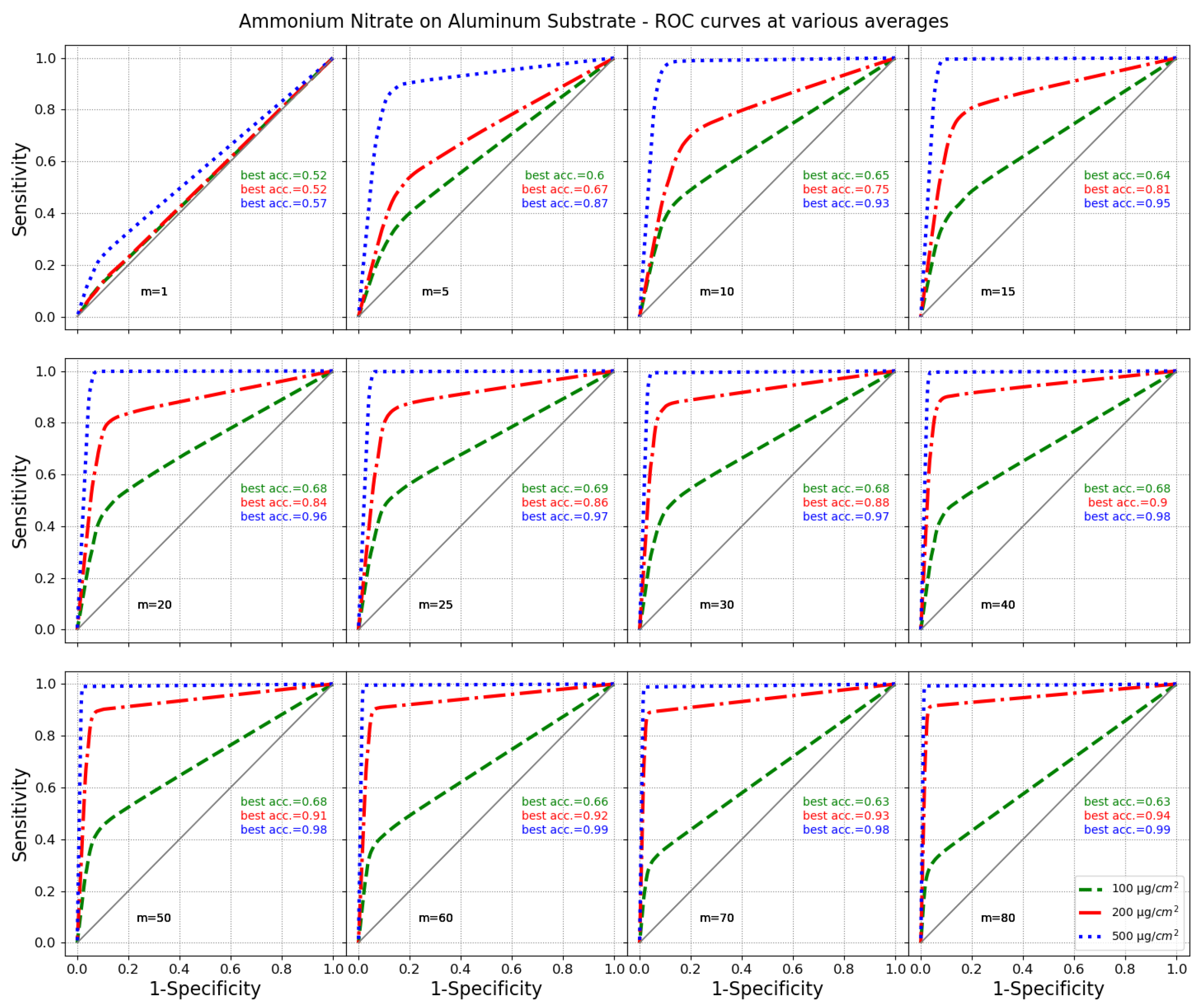
A set of Raman spectra of ammonium nitrate on aluminum substrate at different concentrations has been acquired. This set is composed by 7500 single-shot profiles. The raw spectra are shared as Supplementary Materials. In section Supplementary Materials, file structure and data description can be found. To better rely on the results of the optimization, the whole ensemble was split in two disjoint sets A and B, each composed by 3750 different spectra. Set A was used to train the MC simulation, while Set B was used to test the performances of the classifiers that performed the best on Set A. This procedure ensures the validity of the classifier on independent datasets. In order to consider signals with different SNR, nine different amounts of spectra have been averaged (n = 1, 5, 10, 15, 20, 25, 30, 40, 50, 60, 70, 80). For each dataset, 1000 averaged spectra have been obtained after averaging n random spectra 1000 times. This step was necessary, since otherwise, the quantization error when calculating sensitivity and specificity makes the AUCs and best accuracies not comparable among the different averages for values of AUC close to 1. The spectra were acquired using an UV laser on ammonium nitrate (NHNO) samples deposed over aluminum plates at concentrations of 100, 200 and 500 g/cm. The samples have been printed over aluminum plates to avoid fluorescence interference by Fraunhofer at different concentrations over 2 cm × 2 cm squares. Fraunhofer ICT has manufactured various test samples of inorganic salts on different substrates by using a GeSim Nanoplotter NP 2.1. This drop-on-demand-printer is equipped with a single piezo-driven pipette mounted on a x-y-z stage and delivering droplets of about 300 pL to flat substrates up to 40 × 30 cm. The pipette can be used with multiple inorganic and organic solvents and can be positioned in 10 m steps. The spectroscopic system is based on a 355 nm Nd:YAG laser providing about 10 mJ per pulse at a repetition rate up to 100 Hz (Quantel Centurion+). The target is set 7 m away from an aspheric mirror of 550 mm focal length, F/2.2 (custom made). Atmospheric extinction may be neglected at the given distance and wavelength. The image is focused onto a fiber optic bundle (from CeramOptec) that couples the mirror to a custom spectrometer (F/2.2) specifically designed and manufactured for this application. The spectrum is then focused over an Andor intensified Camera (iStar CCD 334 with UV enhanced photocatode), which is able to intensify the signal only in coincidence with the laser shots, limiting the background illumination and hence the noise of each spectrum. The laser beam is expanded to a spot of 2 cm diameter at the target distance so that the energy density per shot is about 3.1 mJ/cm. Since the laser pulse duration is = 12 ns, the energy density must be compared to the 5600 × = 5.8 mJ/cm of Maximum Permitted Exposure for a single shot [6] so that each pulse can be considered as eye-safe. For multiple shots, however, the total time of deposition must be considered; however, this was not taken into account, and it was assumed that the entire dose was delivered in a time adequate to obtain the eye-safe condition, according to the number of average spectra. The size of the spot was determined to best fit the fiber bundle size. The whole system was designed for standoff Raman detection under eye-safe conditions: for this reason, understanding the performances of the system at low SNRs is crucial to tune it for reliable detections with minimum laser exposure. The best acquisition strategy of spectra accumulated on a CCD over more laser pulses is discussed in [43,44].
3. Results and Discussion
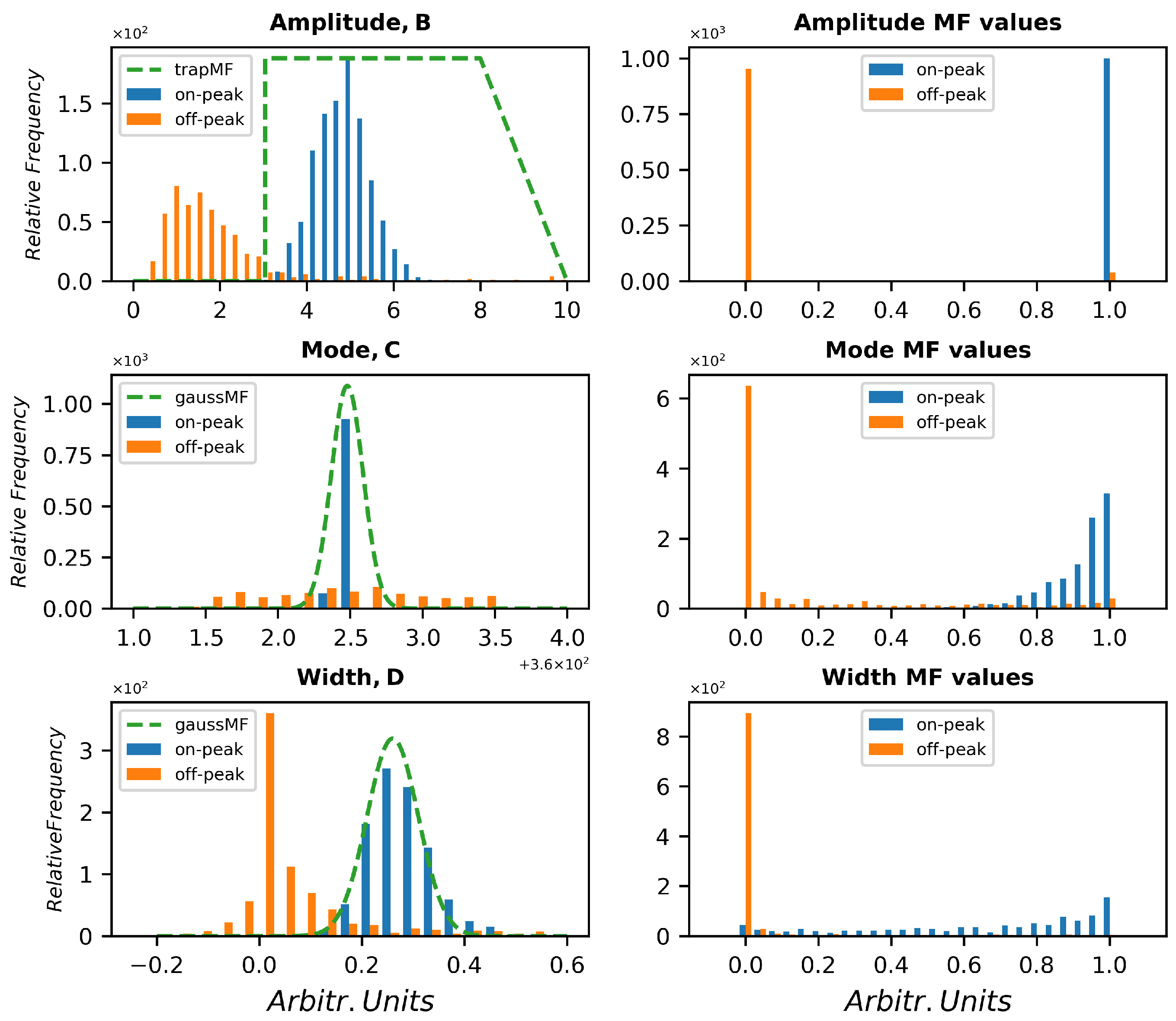
By averaging n random spectra 1000 times, for each concentration, each compound and each substrate, 1000 averaged spectra have been obtained. The off-peak set has been extracted from the same spectra but in a peak-free region in order to use a dataset with the same conditions of sample substrate, background illumination, temperature, laser power and geometry. However, a different set of reference empty spectra can be acquired if needed. Of course, it is important that the acquisition conditions are as similar as possible. The position indices of the off-peak region were shifted before analysis to match the same fitting coordinated as the on-peak samples, while its width was retained. For the specific case under examination, five parameters have been taken into account. Parameters b, c, and d of the fit are distributed as shown in Figure 5. Examples of FMF are plotted in a green dashed line over the distributions of the considered fitting parameters. In the lower panel, the distributions of fuzzy degree of belonging of each parameter are shown with the same color code. All distributions are not entirely disjointed, and little overlap is visible in all histograms, but the fuzzy AND requires all three parameters to fall in an overlapped region to be considered as a false positive or negative, according to its true nature. This considerably lowers the probability of wrong attribution. Of course, the choice of the FMF parameters is crucial to better distinguish between on-peak and off-peak distributions, and the aim of the Monte Carlo simulation is to find the best performing choice.
The parameter c indicates the modal value of the peak (i.e., the center wavelength), while d refers to the peak width. Both parameters are distributed as a bell-shaped distribution, so a Gaussian membership function was adopted. As for b, related to the amplitude of the peak, a bell-shaped function is not suitable, since the absolute value of the amplitude may derive both from the signal collection capabilities (laser energy, optical efficiency) and from the compound quantity, which is unknown. For this reason, it is not possible to lower the membership if the signal is high, because a strong signal could derive from a high quantity of compound; a trapezoidal function has been considered, with very high values (>50) excluded just to cut off outliers and cosmic rays. The left side of the function is connected to the limit of detection: moving the edge to the right lowers the sensitivity of the system, while moving to the left makes the system less selective. Of course, the less the overlap between the on-peak and off-peak parameters distributions, the better the expected performances. For this reason, different concentrations and different SNRs have been taken into account. The Gaussian FMFs can be described by two parameters and the trapezoidal function can be described by just one parameter. The left edge is vertical and acts as a classical set. So, a classifier can be represented by the quintuplet of parameters of the FMFs. Then, the algorithm, as before described, extracted 106 quintuplets (within defined ranges for each parameter) by a uniform random generator, and the performances in terms of AUC and best accuracy were evaluated for each quintuplet. Once the three belonging degrees have been evaluated, a fuzzy AND selects the minimum of these values and determines the overall belonging both for on-peak fit and for off-peak fit. A threshold is hence varied from 0 to 1 to calculate the sensitivity and specificity of the classifier according the threshold and finally the AUC. The best performing classifiers, i.e., those whose AUC exceeded 0.995, were then tested also over the dataset B.
The accuracy varies according to the threshold, and since it is not necessarily correlated to the AUC, a best accuracy with respect to the threshold can be found for each classifier as an independent index. Figure 6 shows that the accuracy and AUC are similar for datasets A and B. The best accuracy can be estimated as 997.5 ± 0.7‰ on dataset A and 997.3 ± 0.8‰ on dataset B. The performances are similar on the two datasets, so we can conclude that the algorithm is sufficiently stable to infer the best parameters on any subset. Figure 7 shows the performances of the best classifiers found at different signal-to-noise ratios, which were obtained as already explained by averaging different amounts of randomly selected single-shot spectra. The procedure described so far allows detecting single peaks within unknown Raman spectra. If this is performed on the most intense Raman line, it allows the identification of groups of molecules or specific groups [45]. If more peaks are evident in the acquired spectrum, the spectrum should be sorted according to the peak rank (i.e., the highest peaks first) and the analysis repeated for each peak, until no attribution is found. Then, supplementary fuzzy rules can be adopted according to the specific needs of the experiment. In this case, the way depicted by Perez Pueyo et al. [32] can be adopted once the positions of the peaks and its degree of belonging have been determined by the fuzzy method illustrated in this work.
Performances with Chemical Contamination
The accuracy of the proposed method was also evaluated when other chemical compounds are mixed with the substance under examination (e.g., mixtures, substrates); peaks near the expected one may alter the performances of the classifier.
Figure 8 shows the expected performances of the classifier where a second peak is overlapped to that under examination. The analysis was conducted by considering the three different parameters entering the classification scheme: peak amplitude, width and position. As these parameters change between the peaks to analyze, the results change, and different performances are expected. For relative peak amplitudes of 0.5, 1 and 2, three different contour plots have been produced. They show the k-score (i.e., the probability of belonging) of the classifier after the fitting procedure and the fuzzy belonging calculations for different relative amplitudes and widths of the peaks. From the figure, it appears that the worst scenario is when the spurious peak is more intense than the true one, and this is pretty obvious. Less intuitive is the fact that also wider peaks lead to bad classifications, and that the worst results are when peaks are shifted by a quantity of about . As demonstrated, a variety of conditions may alter the result of the classifier. If a peak is expected close to the true one, e.g., by a compound already observed or awaited under certain conditions, the fitting procedure could be modified ad hoc, for example, by reducing the fitting region or imposing a different initial guess or by imposing constraints to the parameters. On the other hand, if the true peak is absent, the possibility of false positives may be considered: in this case, the fuzzy membership functions directly provide the probabilities of misclassification according to the amplitude, width and mode of the detected peak. However, the problem of false attribution of a specific peak is mitigated in the perspective of a complete spectrum analysis, where the absence of a peak does not invalidate the classification. This is under study using pigment spectra and will be a subject for future work.
4. Conclusions
The huge amount of works in the field of automated spectral identification witnesses the interest in the field and the difficulties in accomplishing this task. In fact, unanimously shared techniques have not been developed so far and, according to the specific task, many strategies have been proposed. However, fuzzy logic represents a well-performing approach, and it looks promising also for the classification of more complex spectra. Nevertheless, the tuning of FMFs represents a crucial point for the performances of the automated classifier: A Monte Carlo method has been designed and tested to evaluate the performances of a supervised classifier based on fuzzy membership functions of the parameters of a Lorentzian fit applied to the region where a Raman peak is expected. Although the applied laser exposure is so low to maintain the eye-safe conditions, the classifier reached 997.4 ‰ accuracy on 1.5 mg of ammonium nitrate set 7 m away from the receiver. The proposed procedure seems then very promising in detecting substances from low signal-to-noise Raman spectra.
Supplementary Materials
The following supporting information can be downloaded at: https://www.mdpi.com/article/10.3390/chemosensors10080295/s1. The authors decided to make available to anyone who wants real data to train classification algorithms the spectra collected and used for this work. This material is composed by three files (100, 200 and 500 g/cm of ammonium nitrate over aluminum substrate), containing 7500 Raman spectra each, collected as described in the paper, which can be used for comparison and test of different algorithms. The first rows report ancillary information from the camera. The first column represents the wavelength (uncalibrated), and the other columns correspond to a different single-shot spectrum. Calibration can be performed on the laser elastic return and ammonium nitrate main peak, whose Raman shift is reported between 1041 and 1049 cm [38,46,47].
Author Contributions
The authors have equally contributed to the work reported: F.A., S.S. and F.C. All authors have read and agreed to the published version of the manuscript.
Funding
This research was funded by the NATO Science for Peace and Security (SPS) programme, within the project Extras (EXplosive TRAce detection Sensor), grant number G5526.
Institutional Review Board Statement
Not applicable.
Informed Consent Statement
Not applicable.
Data Availability Statement
Data generated during this study are available for download as described in the section Supplementary Materials.
Conflicts of Interest
The authors declare no conflict of interest. The funders had no role in the design of the study; in the collection, analyses, or interpretation of data; in the writing of the manuscript.
Abbreviations
The following abbreviations are used in this manuscript:
| AUC | Area Under Curve |
| ROC | Receiver Operating Characteristic |
| TP | True Positive |
| TN | True Negative |
| FP | False Positive |
| FN | False Negative |
| FMF | Fuzzy Membership Function |
| prct | Percentile |
References
- Dong, R.; Wang, J.; Weng, S.; Yuan, H.; Yang, L. Field deter-mination of hazardous chemicals in public security by using ahand- held Raman spectrometer and a deep architecture-search network. Spectrochim. Acta Part A 2021, 258, 119871. [Google Scholar] [CrossRef]
- Veneranda, M.; Manrique-Martinez, J.A.; Garcia-Prieto, C.; Sanz-Arranz, A.; Saiz, J.; Lalla, E.; Konstantinidis, M.; Moral, A.; Medina, J.; Rull, F.; et al. Raman semi-quantification on Mars: ExoMars RLS system as a tool to better comprehend the geological evolution of martian crust. Icarus 2021, 367, 114542. [Google Scholar] [CrossRef]
- Rousaki, A.; Vandenabeele, P. In situ Raman spectroscopy for cultural heritage studies. J. Raman Spectrosc. 2021, 52, 2178–2189. [Google Scholar] [CrossRef]
- Bernardini, S.; Bellatreccia, F.; Ventura, G.D.; Sodo, A. A Reliable Method for Determining the Oxidation State of Manganese at the Microscale in Mn Oxides via Raman Spectroscopy. Geostand. Geoanal. Res. 2021, 45, 223–244. [Google Scholar] [CrossRef]
- Lui, H.; Zhao, J.; McLean, D.; Zeng, H. Real-time Raman spectroscopy for in vivo skin cancer diagnosis. Cancer Res. 2012, 72, 2491–2500. [Google Scholar] [CrossRef] [Green Version]
- Angelini; Colao, F. Optimization of laser wavelength, power and pulse duration for eye-safe Raman spectroscopy. J. Eur. Opt. Soc.-Rapid Publ. 2019, 15, 2. [Google Scholar] [CrossRef] [Green Version]
- EUR-lex, “CE 25/2006”. 2006. Available online: https://eur-lex.europa.eu/eli/dir/2006/25/oj (accessed on 23 September 2021).
- Mariscotti, M.A. A method for automatic identification of peaks in the presence of background and its application to spectrum analysis. Nucl. Instrum. Methods 1967, 50, 309–320. [Google Scholar] [CrossRef]
- Schmidt-Kaler, T. Automated spectral classification. A survey. Bull. d’Information Cent. DonnéEs Stellaires 1982, 23, 2. [Google Scholar]
- Moss, W.; Wayne, F.; Posey, T.; Peterson, P.C. A mul8variate analysis of the infrared spectra of drugs of abuse. J. Forensic Sci. 1980, 25, 304–313. [Google Scholar] [CrossRef]
- Frankel, D.S. Pattern recognition of Fourier transform infrared spectra of organic compounds. Anal. Chem. 1984, 56, 1011–1014. [Google Scholar] [CrossRef]
- Scott, D.R. Determination of chemical classes from mass spectra of toxic organic compounds by SIMCA pattern recognition and information theory. Anal. Chem. 1986, 58, 881–890. [Google Scholar] [CrossRef]
- Weigel, U.M.; Herges, R. Automatic interpretation of infrared spectra: Recognition of aromatic substitution patterns using neural networks. J. Chem. Inf. Model. 1992, 32, 723–731. [Google Scholar] [CrossRef]
- Shadmehr, R.; Angell, D.; Chou, P.B.; Oehrlein, G.S.; Joffe, R.S. Principal Component Analysis of Optical Emission Spectroscopy and Mass Spectrometry: Application to Reactive Ion Etch Process Parameter Estimation Using Neural Networks. J. Electrochem. Soc. 1992, 139, 907. [Google Scholar] [CrossRef] [Green Version]
- Simmonds, J.E.; Armstrong, F.; Copland, P.J. Species identification using wideband backscatter with neural network and discriminant analysis. ICES J. Mar. Sci. 1996, 53, 189–195. [Google Scholar] [CrossRef] [Green Version]
- Jacobsen, R.H.; Mittleman, D.M.; Nuss, M.C. Chemical recognition of gases and gas mixtures with terahertz waves. Opt. Lett. 1996, 21, 2011–2013. [Google Scholar] [CrossRef] [Green Version]
- Rousaki, A.; Paolin, E.; Sciutto, G.; Vandenabeele, P. Development and evaluation of a simple Raman spectral searching algorithm. Eur. Phys. J. Plus 2021, 136, 620. [Google Scholar] [CrossRef]
- Maquelin, K.; Choo-Smith, L.P.; Endtz, H.P.; Bruining, H.A.; Puppels, G.J. Rapid identification of Candida species by confocal Raman microspectroscopy. J. Clin. Microbiol. 2002, 40, 594–600. [Google Scholar] [CrossRef] [Green Version]
- Wilkins, M.F.; Boddy, L.; Morris, C.W.; Jonker, R.R. Identification of phytoplankton from flow cytometry data by using radial basis function neural networks. Appl. Environ. Microbiol. 1999, 65, 4404–4410. [Google Scholar] [CrossRef] [Green Version]
- Fu, L.; Yang, M.; Braylan, R.; Benson, N. Real-time adaptive clustering of flow cytometric data. Pattern Recognit. 1993, 26, 365–373. [Google Scholar] [CrossRef]
- Zare, H.; Shooshtari, P.; Gupta, A.; Brinkman, R.R. Data reduction for spectral clustering to analyze high throughput flow cytometry data. BMC Bioinf. 2010, 11, 403. [Google Scholar] [CrossRef] [Green Version]
- Boddy, L.; Wilkins, M.F.; Morris, C.W. Pattern recognition in flow cytometry. Cytometry 2001, 44, 195–209. [Google Scholar] [CrossRef]
- Gong, P.; Pu, R.; Yu, B. Conifer species recognition: An exploratory analysis of in situ hyperspectral data. Remote Sens. Environ. 1997, 62, 189–200. [Google Scholar] [CrossRef]
- Yu, B.; Ostland, M.; Gong, P.; Pu, R. Penalized discriminant analysis of in situ hyperspectral data for conifer species recognition. IEEE Trans. Geosci. Electron. 1999, 37, 2569–2577. [Google Scholar] [CrossRef] [Green Version]
- Aardt, J.A.N.V.; Wynne, R.H. Examining pine spectral separability using hyperspectral data from an airborne sensor: An extension of field-based results. Int. J. Remote Sens. 2007, 28, 431–436. [Google Scholar] [CrossRef]
- Pu, R. Broadleaf species recognition with in situ hyperspectral data. Int. J. Remote Sens. 2009, 30, 2759–2779. [Google Scholar] [CrossRef]
- Farinella, G.M.; Gallo, G.; Gueli, A.M.; Stanco, F. Automatic Recognition of Color Pigments from Raman Spectrum Analysis. SIMAI Congr. 2009, 3, 211–221. [Google Scholar]
- Jander, P.; Noll, R. Automated detection of fingerprint traces of high explosives using ultraviolet Raman spectroscopy. Appl. Spectrosc. 2009, 63, 559–563. [Google Scholar] [CrossRef]
- Wang, K.; Guo, P.; Luo, A.L. A new automated spectral feature extraction method and its application in spectral classification and defective spectra recovery. Mon. Not. R. Astron. Soc. 2017, 465, 4311–4324. [Google Scholar] [CrossRef] [Green Version]
- Kukula, K.; Farmer, D.; Duran, J.; Majid, N.; Chatterley, C.; Jessing, J.; Li, Y. Rapid Detection of Bacteria Using Raman Spectroscopy and Deep Learning. In Proceedings of the 11th IEEE Annual Computing and Communication Workshop and Conference, Las Vegas, NV, USA, 27–30 January 2021; pp. 796–799. [Google Scholar]
- Soneira, M.J.; Perez-Pueyo, R.; Ruiz-Moreno, S. Raman spectra enhancement with a fuzzy logic approach. J. Raman Spectrosc. 2002, 33, 599–603. [Google Scholar] [CrossRef]
- Perez-Pueyo, R.; Soneira, M.J.; Ruiz-Moreno, S. A fuzzy logic system for band detection in Raman spectroscopy. J. Raman Spectrosc. 2004, 35, 808–812. [Google Scholar] [CrossRef]
- Tutzó, M.C.; Perez-Pueyo, R.; Soneira, M.J.; Moreno, S.R. Fuzzy logic: A technique to Raman spectra recognition. J. Raman Spectrosc. 2006, 37, 1003–1011. [Google Scholar] [CrossRef]
- Castanys, M.; Soneira, M.J.; Perez-Pueyo, R. Automatic Identification of Artistic Pigments by Raman Spectroscopy Using Fuzzy Logic and Principal Component Analysis. Laser Chem. 2006, 2006, 018792. [Google Scholar] [CrossRef]
- Dina, N.E.; Gherman, A.M.R.; Colniță, A.; Marconi, D.; Sârbu, C. Fuzzy characterization and classification of bacteria species detected at single-cell level by surface-enhanced Raman scattering. Spectrochim. Acta Part A 2021, 247, 119–149. [Google Scholar] [CrossRef] [PubMed]
- Alamaniotis, M.; Jevremovic, T. Hybrid fuzzy-gene8c approach integrating peak identification and spectrum fitting for complex gamma-ray spectra analysis. IEEE Trans. Nucl. Sci. 2015, 62, 1262–1277. [Google Scholar] [CrossRef]
- Perez-Pueyo, R.; Soneira, M.J.; Castanys, M.; Ruiz-Moreno, S. Fuzzy approach for identifying artistic pigments with Raman spectroscopy. Appl. Spectrosc. 2009, 63, 947–957. [Google Scholar] [CrossRef]
- Chirico, R.; Almaviva, S.; Colao, F.; Fiorani, L.; Nuvoli, M.; Schweikert, W.; Schnürer, F.; Cassioli, L.; Grossi, S.; Murra, D.; et al. Proximal Detection of Traces of Energetic Materials with an Eye-Safe UV Raman Prototype Developed for Civil Applications. Sensors 2016, 16, 8. [Google Scholar] [CrossRef]
- Wei, D.; Chen, S.; Liu, Q. Review of fluorescence suppression techniques in Raman spectroscopy. Appl. Spectrosc. Rev. 2015, 50, 387–406. [Google Scholar] [CrossRef]
- Chiuri, A.; Angelini, F. Fast Gating for Raman Spectroscopy. Sensors 2021, 21, 2579. [Google Scholar] [CrossRef]
- Ross, T.J. Fuzzy Logic with Engineering Applications; John Wiley & Sons: Hoboken, NJ, USA, 2005. [Google Scholar]
- Arslan, A.; Kaya, M. Determination of fuzzy logic membership functions using gene8c algorithms. Fuzzy Sets Syst. 2001, 118, 297–306. [Google Scholar] [CrossRef]
- Angelini, F.; Frischia, S.D.; Chiuri, A.; Colao, F. Maximization of Raman signal in standoff detection under eye-safe conditions. Counterterrorism Crime Fight. Forensics Surveill. Technol. III 2019, 11166, 1116609. [Google Scholar]
- Frischia, S.D.; Chiuri, A.; Angelini, F.; Colao, F. Optimization of signal-to-noise ratio in a CCD for spectroscopic applications. In Proceedings of the 15th European Workshop on Advanced Control and Diagnosis, Bologna, Italy, 21–22 November 2019. [Google Scholar]
- Reiser, O.L. Physics, Probability, and Multi-Valued Logic. Philos. Rev. 1940, 49, 662–672. [Google Scholar] [CrossRef]
- Sadate, S.; Farley, C., III; Kassu, A.; Sharma, A. Standoff Raman spectroscopy of explosive nitrates Using 785 nm Laser. Am. J. Remote Sens. 2015, 3, 1–5. [Google Scholar] [CrossRef]
- Hadi, N.M.; Mohammad, M.R.; Abdulzahraa, H.G. Standoff Raman Detection of Explosive Materials Using a Small Raman Spectroscopy System. Al-Nahrain J. Sci. 2017, 20, 60–66. [Google Scholar] [CrossRef]
Figure 1.
Left: Correlation coefficient (red) and Euclidean distance (black) between a reference spectrum and the same spectrum with added synthetic noise for different signal-to-noise amounts. Right: The reference spectrum (orange) and the same spectrum with added synthetic noise (blue) for the case SNR = 9.26. The black dashed box indicates the region where the noise is estimated as the standard deviation of the signal.

Figure 2.
Peak fitting with a Lorentzian curve in a region where a peak is present (red) and where no peaks are present (blue). Parameters (a = 501.14, b = 6.74, c = 362.59, d = 0.15) refer to the red curve.
Figure 2.
Peak fitting with a Lorentzian curve in a region where a peak is present (red) and where no peaks are present (blue). Parameters (a = 501.14, b = 6.74, c = 362.59, d = 0.15) refer to the red curve.

Figure 3.
Fuzzy membership functions and degree of belonging of the variable P. The value assumed by the FMF at abscissa P represents the belonging to that set. In this case, while P has belonging 0 in the classic dataset (red), it shows a belonging of 0.226 to the Gaussian FMF function (blue), 0.300 to the triangular FMF function, and 0.375 to the trapezoidal FMF (black).

Figure 4.
Flow chart of the algorithm for recognition of a single peak. In our case, N = M = 1000 spectra.
Figure 4.
Flow chart of the algorithm for recognition of a single peak. In our case, N = M = 1000 spectra.

Figure 5.
Distribution of the parameters B, C, D of the Lorentzian fit together with hypothetic fuzzy membership functions (top) and distribution of the fuzzy belonging degrees of each parameter according to the FMFs shown (bottom).
Figure 5.
Distribution of the parameters B, C, D of the Lorentzian fit together with hypothetic fuzzy membership functions (top) and distribution of the fuzzy belonging degrees of each parameter according to the FMFs shown (bottom).

Figure 6.
Distribution of the accuracy and AUC for the best 1400 classifiers on dataset A and B.

Figure 7.
AUCs and best accuracies for ammonium nitrate over aluminum substrates for 100, 200 and 500 g/cm and for signal averaged over a different number of single-shot spectra.
Figure 7.
AUCs and best accuracies for ammonium nitrate over aluminum substrates for 100, 200 and 500 g/cm and for signal averaged over a different number of single-shot spectra.

Figure 8.
Performances of the classifier when a spurious peak is overlapped in the fitting region to the true one. The color refers to the k-score expressing the overall belonging of the peak. Calculations have been performed after synthetic noise was added to the peak for an SNR of 10.
Figure 8.
Performances of the classifier when a spurious peak is overlapped in the fitting region to the true one. The color refers to the k-score expressing the overall belonging of the peak. Calculations have been performed after synthetic noise was added to the peak for an SNR of 10.

Publisher’s Note: MDPI stays neutral with regard to jurisdictional claims in published maps and institutional affiliations. |
© 2022 by the authors. Licensee MDPI, Basel, Switzerland. This article is an open access article distributed under the terms and conditions of the Creative Commons Attribution (CC BY) license (https://creativecommons.org/licenses/by/4.0/).
Share and Cite
MDPI and ACS Style
Angelini, F.; Santoro, S.; Colao, F. Chemical Identification from Raman Peak Classification Using Fuzzy Logic and Monte Carlo Simulation. Chemosensors 2022, 10, 295. https://doi.org/10.3390/chemosensors10080295
AMA Style
Angelini F, Santoro S, Colao F. Chemical Identification from Raman Peak Classification Using Fuzzy Logic and Monte Carlo Simulation. Chemosensors. 2022; 10(8):295. https://doi.org/10.3390/chemosensors10080295
Chicago/Turabian StyleAngelini, Federico, Simone Santoro, and Francesco Colao. 2022. "Chemical Identification from Raman Peak Classification Using Fuzzy Logic and Monte Carlo Simulation" Chemosensors 10, no. 8: 295. https://doi.org/10.3390/chemosensors10080295
Note that from the first issue of 2016, this journal uses article numbers instead of page numbers. See further details here.