
Estimating Copula-Based Extension of Tail Value-at-Risk and Its Application in Insurance Claim


1
Statistics Research Division, Institut Teknologi Bandung, Bandung 40132, Indonesia
2
Analysis and Geometry Research Division, Institut Teknologi Bandung, Bandung 40132, Indonesia
*
Author to whom correspondence should be addressed.
Risks 2022, 10(6), 113; https://doi.org/10.3390/risks10060113
Submission received: 24 April 2022
/
Revised: 23 May 2022
/
Accepted: 24 May 2022
/
Published: 30 May 2022
Abstract
:Dependent Tail Value-at-Risk, abbreviated as DTVaR, is a copula-based extension of Tail Value-at-Risk (TVaR). This risk measure is an expectation of a target loss once the loss and its associated loss are above their respective quantiles but bounded above by their respective larger quantiles. In this paper, we propose nonparametric estimators for DTVaR and establish their property of consistency. Moreover, we also propose the variability measure around this expected value truncated by the quantiles, called the Dependent Conditional Tail Variance (DCTV). We use this measure for constructing confidence intervals of the DTVaR. Both parametric and nonparametric approaches for DTVaR estimations are explored. Furthermore, we assess the performance of DTVaR estimations using a proposed backtest based on the DCTV. As for the numerical study, we take an application in the insurance claim amount.
1. Introduction
In actuarial science, several risk measures have been proposed; the two most well-known are the Value-at-Risk (VaR) and the Tail Value-at-Risk (TVaR). Several authors have proposed (or compared) nonparametric estimators for VaR and TVaR; see Chang et al. (2003); Brazauskas et al. (2008); Kaiser and Brazauskas (2006); Methni et al. (2014); Dutta and Biswas (2018) and Shen et al. (2019).
In particular, Chang et al. (2003) introduced three types of VaR nonparametric estimation methods and their corresponding confidence intervals. Brazauskas et al. (2008) and Kaiser and Brazauskas (2006) proposed point and interval estimators for TVaR, as well as proved the consistency of the point estimator. Methni et al. (2014) combined nonparametric kernel methods with extreme-value statistics to find the estimator for TVaR. Dutta and Biswas (2018) compared the performance of nonparametric estimators of TVaR for varying p, namely the empirical estimator, kernel-based estimator, Brazauskas et al.’s estimator, tail-trimmed estimator by Hill, Yamai and Yoshiba’s estimator and the filtered historical method. Shen et al. (2019) established empirical likelihood–based estimation with high-order precision for TVaR.
Several extensions of TVaR have also been developed. Jadhav et al. (2013); Wang and Wei (2020); Bairakdar et al. (2020) and Bernard et al. (2020) have modified TVaR by introducing a fixed boundary, instead of infinity, for values beyond the quantile (i.e., VaR). In particular, Jadhav et al. (2013) named the modified risk measure as Modified TVaR (MTVaR). Meanwhile, another extension of TVaR, called Copula TVaR (CTVaR), was suggested by Brahim et al. (2018), in which, they estimate a target loss1 by involving another dependent or associated loss.
Motivated by the work of Jadhav et al. (2013) and Brahim et al. (2018); Josaphat and Syuhada (2021) proposed an alternative coherent risk measure that is not only “considering a fixed upper bound of loss beyond VaR” but also “taking into account an associated loss”, called Dependent TVaR (DTVaR). Moreover, Josaphat et al. (2021) proposed an optimization method for DTVaR by applying two metaheuristic algorithms: Spiral Optimization (SpO) and Particle Swarm Optimization (PSO). When we calculate an MTVaR estimate, it will subtract the number of losses beyond VaR and thus make this estimate smaller than the corresponding TVaR. This is a good feature in risk modeling. We argue that this estimate must also be accompanied by an associated risk since this risk scenario occurs in practice; see, for instance, Zhang et al. (2019) and Kang et al. (2019).
The DTVaR can comprehend the connection between bivariate losses and help us to optimally position our investments and enlarge our financial risk protection (Josaphat and Syuhada 2021). In other words, employing the suggested risk measure will enable us to avoid non-essential additional capital allocation while not ignoring other risks associated with the target risk. In this paper, we propose two nonparametric estimators for the risk measure of DTVaR by following the approaches of Brazauskas et al. (2008) and Jadhav et al. (2013). These estimators are proven to be consistent.
Although the DTVaR serves crucial information on the tail distribution of the target loss, the necessity for other risk measures came up in competitive and unpredictable market environments. Principally, realizing that the DTVaR, being the tail mean, is not able to capture the tail variability, we propose a second tail moment or variance in the tail distribution truncated by two pair of VaRs that is called Dependent Conditional Tail Variance (DCTV). This measure can concatenate the dissemination in the tail. Moreover, the DCTV can be considered a generalization of Conditional Tail Variance (CTV) proposed by Furman and Landsman (2006). Using DCTV, we are able to prove the asymptotic normality of DTVaR and even derive confidence intervals for the DTVaR estimators. Just as Righi and Ceretta (2015) used CTV for the backtesting of TVaR estimations using the bootstrap method, we also use DCTV for the backtesting of DTVaR estimations.
The rest of the paper is organized as follows. In Section 2, we briefly explain the novel risk measure of dependent tail VaR. The nonparametric estimation of DTVaR is discussed in Section 3, whereas the truncated variance, called the dependent conditional tail variance, is presented in Section 4. Section 5 presents the parametric estimate of DTVaR in a Pareto case. The choice of the contraction parameters that appear in the definition of DTVaR is considered in Section 6. Conclusions are discussed in Section 7. All mathematical proofs are deferred to Appendix A.
2. The Dependent Tail Value-at-Risk
Let be an atomless probability space, and be the set of real integrable random variables (i.e., random variables with finite means) defined on A risk measure is a functional
Consider that X and Y are two random losses that are dependent and have marginal distribution functions and . Provided a value generally close to one, the VaR of X at a probability level is the quantile of for this level. Mathematically, the VaR is defined as follows:
Based on this definition, we can note that the VaR does not consider information after the quantile of interest, only the point itself. Moreover, despite its simplicity and ease of implementation, VaR has the shortcoming of not being a coherent risk measure in the sense of Artzner et al. (1999). The TVaR at probability level is then the expectation of X once X is above the VaR for this level, i.e., an extreme loss. Formally, Formulation (2) defines TVaR.
Note that in (2) is the significance level for TVaR.
As we state in Section 1; Josaphat and Syuhada (2021) proposed another risk measure as a generalization of TVaR that not only considers the information about the potential size of the loss X between two quantiles but also takes into account the excess of another loss Y that is associated with X. Formally, Formulation (3) defines DTVaR.
where Y is another loss that is associated with X (or X depends on Y), , and . Here, and denote the probability level and excess level, respectively. Moreover, X is called the target loss, whereas Y is called the associated loss. In the sequel, two lemmas related to the DTVaR are given.
Lemma 1
(Josaphat and Syuhada 2021). Let X and Y be two random losses with a joint probability function . Let and be specified numbers. The Dependent Tail VaR (DTVaR) of X given values beyond its VaR up to a fixed value of losses and a random loss Y is given by
where and .
In practice, a joint probability function is difficult to find unless a bivariate normal distribution is assumed. For the case of joint exponential distribution, we may refer to Kang et al. (2019) for Sarmanov’s bivariate exponential distribution. In most cases, two or more dependent losses rely on a copula in order to have an explicit formula of its joint distribution.
Lemma 2
(Josaphat and Syuhada 2021). Let X and Y be two random losses with a joint distribution function represented by a copula C. Let and be specified numbers. The Dependent Tail VaR (DTVaR) of X given values beyond its VaR up to a fixed value of losses and a random loss Y is given by
where denotes the quantile function of X, and .
The following property applies to DTVaR. The property states that the DTVaR is a law-invariant convex risk measure.
Property 1.
The Dependent Tail VaR (DTVaR) is a law-invariant risk measure.
3. The Estimation of DTVaR
When dealing with real data, it is not always easy for us to know the distribution of the data, even if we use software for fitting distribution. As a result, estimating DTVaR is also not easy. To avoid the difficulty of the parametric estimation of DTVaR, we propose a nonparametric one.
We propose two nonparametric estimators of the DTVaR. The first empirical estimator of is defined as follows. Let be a collection of random vectors with size m, where and are independently and identically distributed (iid) random losses, respectively. Suppose that denotes the corresponding empirical joint distribution function, which is given by
where denotes the indicator function. In addition, suppose that and denote the empirical marginal distribution functions of iid and iid , which are given by
Suppose that and denote the unknown distribution functions of X and Y.
If the vectors are rearranged by considering the ascending order of , then we obtain new vectors . It is obvious that are order statistics of . However, the statistics , , are not necessarily order statistics of . Furthermore, the quantiles , , and , respectively, can be consistently estimated by
where , and . Hence, for , the estimator is given by
Consider a square originating from two intervals . Subdivide each of both intervals into m subintervals and m subintervals so that we obtain small squares . When and , then we have that and . Similarly, when and , then we have that and . Clearly, , , and . Hence,
Note that, in (7), we do not sum but paired with . To simplify the notation and computation, we sum by applying the indicator function ; thus, we obtain
Next, note that
where and , respectively, denote the realizations of and , whilst,
From (8) and (9), we obtain
for all and
Note that, in a similar and simpler way, it can be shown that an estimator of MTVaR (proposed by Jadhav et al. 2013) is given by
for all and . Note that . If we adjust the index i in (11) to index q, then can be rewritten as (see Jadhav et al. 2013)
where and denotes the smallest integer that is larger than
Following the derivation method of the estimator in (12), we obtain
where ,
r is the number of s paired with that does not satisfy The estimator given in (13) may be improved by considering a smoothed version, which is the second estimator, as follows:
where .
In the following theorem, we prove the consistency of DTVaR estimators.
4. The Dependent Conditional Tail Variance and Confidence Intervals
In addition to the TVaR, some authors also consider the variability of the loss in the tail of the distribution. The notion is that, in spite of its practicality and desired properties, the TVaR only picks up the average loss in the tail and forsakes its variability, and thus it makes sense to concatenate the second tail moment or the variance in the tail distribution. In this regards, Furman and Landsman (2006) put forward the Tail Variance Premiun (TVP) that contains Conditional Tail Variance (CTV),
where the last term is called the CTV. Moreover, Righi and Ceretta (2015) used the square root of the CTV, instead of ordinary variance, for the backtesting of TVaR estimation using the bootstrap method.
Motivated by the CTV proposed by Furman and Landsman (2006), we propose a Dependent Conditional Tail Variance (DCTV) of target loss X associated with another loss Y,
Thus, DCTV is a variability or dispersion measure around DTVaR truncated by the VaRs of target loss and associated loss. In addition, since DTVaR is a generalization of TVaR, then DCTV is also a generalization of CTV.
The DCTV of the target loss X computed under a fixed conditional probability with respect to the associated loss Y is given in the following lemma.
Lemma 3.
Let X and Y be two random losses with a joint distribution function represented by a copula C. Let and be specified numbers. The Dependent Conditional Tail Variance (DCTV) of X given values beyond its VaR up to a fixed value of losses and a random loss Y is given by
where is given in (5).
4.1. The Estimation of DCTV
Following the derivation method of the estimators and in (13) and (14), we obtain two estimators for , namely,
and
where .
In the following theorem, we prove the consistency of DCTV estimators.
4.2. Confidence Intervals for DTVaR
It is obvious that the estimators in (13) and (14) are point estimators for DTVaR. The next step is to construct point-wise confidence intervals for DTVaR. We derive the (point-wise) confidence intervals, whose construction is based on the following asymptotic result.
Theorem 3.
Let and contraction parameters a and d be fixed. Let the distribution function be continuous at the points and . Then, for , we have
where and are given in (5) and (16). In particular, statement (19) holds for any finite contraction parameters if the distribution function is continuous everywhere on the real line.
Using (19), we derive the following level asymptotic confidence intervals for the DTVaR,
where is the percentile of the standard normal distribution. The truncated variance DCTV is unknown but has been estimated empirically from DCTV estimators given in (17) and (18). Hence, we have the following level asymptotic confidence intervals for the DTVaR,
Remark 1.
We apply the confidence intervals (20) for DTVaR backtesting using the bootstrap method in Section 6.2.
5. Parametric Estimation under FGM Copula
In this section, we find parametric estimates for the DTVaR at any given and specified contraction parameters under a Pareto distribution by using the Maximum Likelihood Estimation (MLE) method of Pham et al. (2019). However, before calculating the estimates, we take the following steps:
- Derive the expression of the DTVaR for the Pareto distribution;
- Calculate the parametric estimates of the distribution parameters of random samples and , each of which is assumed to be a Pareto distribution.
Moreover, we show that the DTVaR, when we consider the correlation (or dependence) between positive quadrant dependent (PQD) losses, is larger than the TVaR. That means, for , then
Note that, in the Negative-Quadrant-Dependent (NQD) losses, we have the reverse of Inequality (21). In particular, also note that is the joint significance level (j.s.l.) for the DTVaR in (21). We use the j.s.l. for assessing the performance of DTVaR estimation.
Now, we derive the expression for the DTVaR for a Pareto distributed loss associated with another loss joined by a Farlie–Gumbel–Morgenstern (FGM) copula that is defined as . We are aware that the FGM copula introduces only light dependence. However, it admits positive as well as negative dependence between a set of random variables. The FGM copula is often used in applications to describe dependence structures due to its tractability and simplicity (see, for instance, Barges et al. 2009; Chadjiconstantinidis and Vrontos 2014; and Jiang and Yang 2016).
Suppose that X is a Pareto random loss with parameter . Suppose also that our dependent (associated) random loss Y is following Pareto distribution with parameter . The distribution function of X and Y are, respectively, for , and for . Their inverses are easy to find and thus their VaRs are as well, which are and .
The risk measure DTVaR formula for X given Y, under the FGM copula, may be found by using Lemma 2.
Lemma 4.
Let X and Y be two Pareto distributed random variables with parameters and with parameter . Suppose that the joint distribution of X and Y are defined by a bivariate FGM copula as follows:
with . Then, the DTVaR of X given Y at levels α and is
where θ denotes the dependence (or Copula) parameter between X and Y, the copula ,
The corresponding parametric estimate of DTVaR in (22) is then found by replacing unknown parameters and with their respective estimates. That is, we have
Example 1.
Lethave a Pareto distribution with parameters and , i.e., . Let Y be another Pareto random loss that also has a Pareto distribution and associates with . Both Figure 1 and Figure 2 present the DTVaR estimates for various FGM copula parameters and , along with the TVaR estimates. Consider the bivariate losses . For each couple , we set , and , respectively (see Figure 1a). The selection of parameters corresponds, respectively, to the strong, medium and weak dependences. In Figure 1a, the comparison of the riskiness of and is presented. Notice that the risk measures of the TVaR of at level α are the same in the three cases. Furthermore, note that DTVaR coincides with TVaR in the independence case (), whereas DTVaR is exactly the same as CTVaR when . The DTVaR of the loss is higher than those of and , respectively, i.e., is riskier than and In Figure 1b, it is shown that both DTVaR and TVaR of are located above the VaR of for the same probability level α. We can see that the DTVaR estimates are always larger than the TVaR estimates when the copula parameters are positive, whereas the DTVaR estimates are always smaller than the TVaR estimates when the opposite occurs (see Figure 2). Therefore, these results are in accordance with the statement (21) and its reverse.
6. Data Analysis
We have used the data of one-year vehicle insurance policies from Macquarie University (2005). This data set is based on one-year vehicle insurance policies taken out in 2004 or 2005. There are 67,856 policies, of which, 4624 (6.8%) had at least one claim. To be clear, the vehicle values written in the source (data set) are values in USD 10,000 s. Out of 4624 policies, there are six observations whose vehicle value is 0. We do not include these six observations in the calculation of DTVaR estimations. Therefore, the data size is . Suppose that the target loss X is the insurance claim amount and the associated loss Y is the vehicle value.
Table 1 provides summary statistics on the claim amount and vehicle value. We can find that both the claim amount and vehicle value have positive skewness, namely 5.0470 and 1.8614, respectively. Moreover, the respective kurtosis of the claim amount and vehicle value is significant when higher than 3. Kurtosis values above 3 (43.3102 and 9.9344) indicate that, relative to a normal distribution, more probability tends to be at points away from the mean than at points near the mean. This is confirmed by Figure 3. Moreover, Figure 3c shows the box plot of the data of the claim amount, depicting that there are 758 outliers in the right tail.
In this section, we compute the parametric estimates of DTVaR. Before comparing the parametric and nonparametric (empirical) estimates of DTVaR, we compute the estimators of DTVaR suggested in Section 3.
Our empirical analysis supports the claim that the suggested risk measure does not underestimate or overestimate the actual risk for and various . Thus, DTVaR is quite meaningful. However, the DTVaR does not necessarily estimate the actual risk properly when the contraction parameters and . This is not surprising, because of the presence of the excess level (other than the probability level ), together with contraction parameter d, which also contributes to the DTVaR estimation. We employ the hypothesis testing procedure (backtesting) to verify this claim empirically. In the future, we need to concurrently estimate and , which can optimize DTVaR using numerical optimization so that DTVaR estimates the actual risk properly.
6.1. Parametric Preliminary Results
By using the MLE method, we obtain the results that X and Y are both Pareto distributed with parameter estimates that are for X, and , for Y. In particular, for X, the estimation of parameters is very likely to be influenced by the large number of outliers in the claim amount. Again, by using the MLE method, we obtain the estimate of FGM copula parameter .
Consider the bivariate loss . For , we have . Furthermore, note again that DTVaR coincides with CTVaR when . In Figure 4a, it is evident that both DTVaR and DTVaR estimates are located between the estimates of VaR with different probability levels. It is interesting to note that DTVaR is smaller than both DTVaR and TVaR (see Figure 4a–c). This fact indicates that DTVaR is much more flexible than TVaR and CTVaR, i.e., DTVaR can be set as equal to or less than CTVaR, or even less than TVaR, by carefully determining the parameters a and d. Furthermore, the results in Figure 4b,c show the same pattern as the results in Figure 1, i.e., the estimates of DTVaR are larger than those of TVaR, which is due to the positive copula parameter estimate.
6.2. Backtesting
In the backtesting for the DTVaR, we are interested in the size of the discrepancy between the claims above the VaR estimate and the estimate of the DTVaR when VaRs violation occurs. A VaRs violation occurs when the actual loss is larger than the estimated figures at specified probability and excess levels. These discrepancies can be positive, negative or zero. We assume that these discrepancies (also called residuals) are iid, conditioned on claims that are larger than the VaRs estimates. We propose an adaptation (generalization) of the Righi and Ceretta (2015) procedure. This approach is based on series r, which represents the residual exceedances over the VaR, i.e., the violations standardized by the DTVaR estimate and the DCTV estimate of claim X. Given a probability level and an excess level , we can formally represent r by formulation
It is clear that we consider the standard deviation truncated by the VaRs, which is the square root of the presented measure DCTV. Similar to Righi and Ceretta (2015), under the null hypothesis, r has a zero mean, against the alternative that the mean of r is positive or negative. This alternative hypothesis represents the real danger, which is underestimating or overestimating loss. Once there is a violation, we take into consideration the information regarding the quantile that the VaR is calculated rather than all of the distribution. Instead of using the p-value for the hypothesis, we use the confidence interval (CI) at a confidence level , which is calculated based on 1000 bootstrap samples (see Righi and Ceretta 2015 and Jadhav et al. 2013). We reject the null hypothesis when the resulting bootstrap CI contains 0.
6.3. Result Analysis
We have estimated the DTVaR and DCTV based on data of one-year vehicle insurance policies. Figure 5, Figure 6 and Figure 7 and Table 2, Table 3, Table 4 and Table 5 present estimates of the DTVaR and DCTV of the respective probability levels and excess levels for various values of a and d. In Table 3, Table 4 and Table 5, the abbreviations LCL and UCL denote the lower confidence level and upper confidence level of a CI at confidence level . Note that, according to CIs (20), we have
where are given in (13) and (14), and are given in (17) and (18).
In particular, Table 2 shows the number as well as the percentage of violations of DTVaR estimations, i.e., the assessment of accuracy for the DTVaR estimates. The assessment is carried out by first observing the joint significance level. For example, in Table 2 (first row, first column), a 0.95% joint significance level (j.s.l.) is lower than 10%. This means that the DTVaR estimates are quite accurate. In the second place, by calculating the number of violations against the , and , we obtain the percentages of violations of 1.34%, 1.41% and 2.81%, respectively. The number 1.34% is obtained from the division between 62 and 4618, where 62 is the number of violations and 4618 is the total number of observations. Essentially, the number of violations is the number of observations located outside of the critical value, i.e., greater than the DTVaR estimate. These computations are shown for different and . Note that, for various and , the differences between j.s.l. and the percentage of violations for the parametric estimates are always greater than those for the two nonparametric ones. This result implies that we should look for another distribution that is more fit for the variable of the claim amount. We also obtain the fact that the smaller the excess level , the smaller the differences between j.s.l. and the percentage of violations. This implies that both nonparametric estimators accurately estimate the DTVaR at an excess level of .
In Figure 5, we can see that the estimates of DTVaR are relatively larger than those of TVaR. Those relatively large DTVaR estimates are highly probably influenced by the number of outliers (758 observations). In Figure 6a, it can be seen that both first and second estimates of DTVaR relatively nearly coincide. Furthermore, we can see in Figure 6b,c that both first and second estimates of DTVaR are larger than the corresponding estimates of DCTV.
From Table 3, we can see that, for , all bootstrap CIs contain 0. We can see similar results from Table 4, where, for , all bootstrap CIs also contain 0. These results indicate that the null hypothesis cannot be rejected, which supports the suggested estimation method for and , that is, there is no underestimation or overestimation of the target loss (claim amount). From both tables, as the values of probability and excess levels increase, estimates of the DTVaR also increase, which is quite obvious. It is interesting to note that, in Table 4, when , estimates of DTVaR are greater at than at , but when , estimates of DTVaR are smaller at than at .
Table 5 shows different results from Table 3 and Table 4. Although we can see that the larger the values of probability and excess levels, the larger the estimates of the DTVaR, it is interesting to note that, for several pairs , estimates of DTVaR fail the backtest. These results indicate that DTVaR estimation is complicated. To overcome this problem, we suggest in the future that the contraction parameters a and d be determined by performing DTVaR optimization so that DTVaR can properly estimate risk. Note that LCL, LCL, UCL and UCL in Table 2, Table 3, Table 4 and Table 5 are calculated using Formulas (25) and (26).
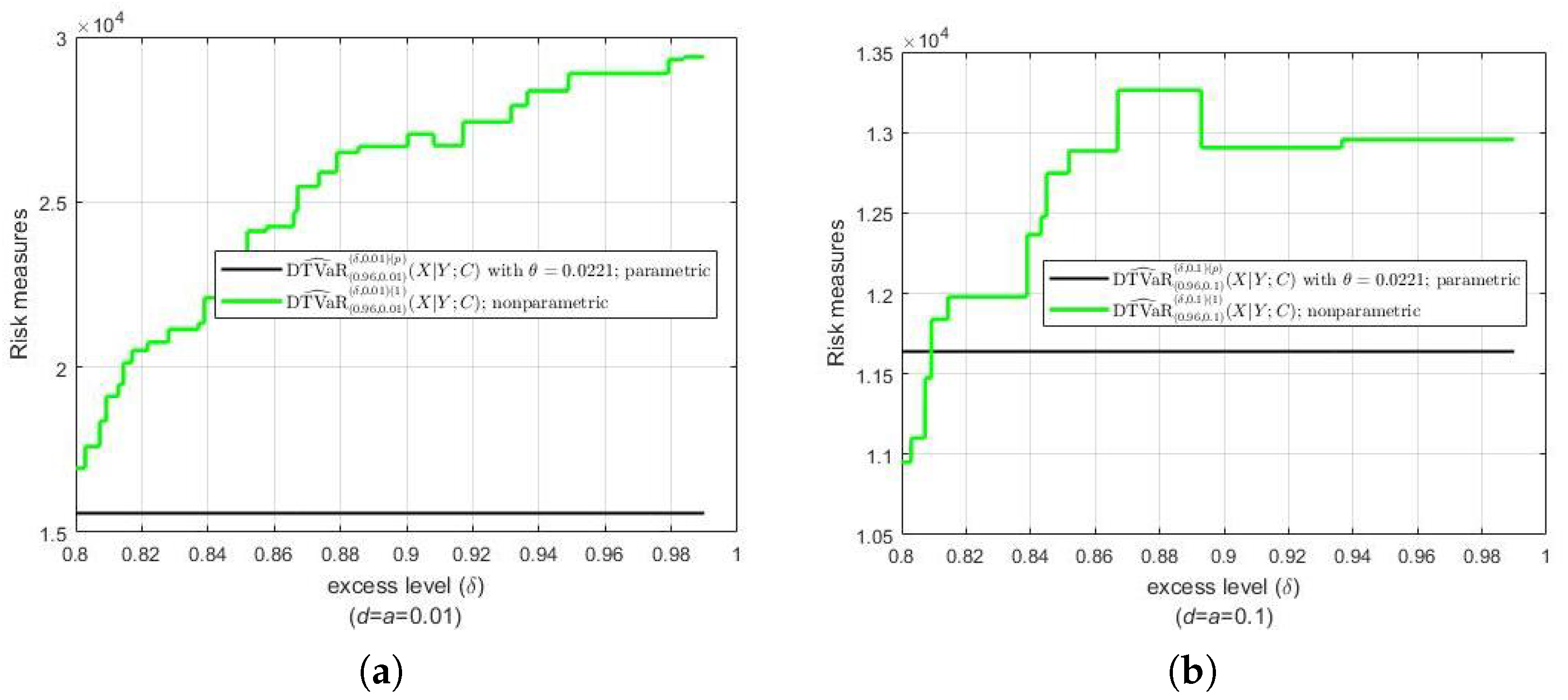
Figure 7 presents two different results regarding the difference between the parametric estimates of the DTVaR and its nonparametric estimates. When the contraction parameter , we can see in Figure 7a that the differences between the two are relatively large, and even very large for values approaching 1. However, for , the differences between the two estimates are relatively small (see Figure 7b).
7. Conclusions
In this paper, we study a recent coherent risk measure called Dependent Tail Value-at-Risk (DTVaR) initially proposed by Josaphat and Syuhada (2021), and suggest the estimators. We have proven the consistency of the estimators. Moreover, we also derive a parametric estimate of DTVaR for Pareto distribution under an FGM copula. For the backtesting of DTVaR estimation, we have also suggested a novel variability measure called Dependent Conditional Tail Variance (DCTV), instead of an ordinary variance of the target loss, along with the estimators for DCTV. Additionally, using DCTV, we establish the asymptotic normality of DTVaR estimators and construct confidence intervals for DTVaR.
We found that the nonparametric estimators are more accurate at estimating DTVaR than the parametric estimator. This result implies that we should look for other distributions that are more fit for the variable of the claim amount. Moreover, we will find the DTVaR formulas of the claim amount for exponential and lognormal distributions since the application of both distributions covers actuarial science. Then, we will again compare the accuracy of the DTVaR parametric estimators for exponential and lognormal distributions to the counterpart nonparametric estimators. In the empirical results, the bootstrap CIs in the backtesting procedure have also confirmed that the estimates of the DTVaR do not underestimate or overestimate the actual loss when or . However, the DTVaR does not necessarily estimate the actual risk properly when the contraction parameters and . The limitation in our research is that the data of the claim amount contain a large number of outliers, i.e., 16.41% of all observations. This situation may be the reason for why DTVaR estimates are relatively much larger than both DTVaR and TVaR estimates. In this case, if the risk measure of DTVaR is employed to the insurance company, this will push the company to prepare a very large extra fund, which is not necessary. In the future, we will apply Archimedean copulas, such as Clayton and Gumbel, to DTVaR. Archimedean copulas are broadly used in implementations due to their easy form, a diversity of dependence structures and other “nice” properties (Brahim et al. 2018).
Author Contributions
Conceptualization, K.S.; methodology, K.S., O.N. and B.P.J.; software, B.P.J.; validation, K.S.; formal analysis, K.S. and B.P.J.; investigation, B.P.J.; resources, K.S.; data curation, B.P.J.; writing—original draft preparation, K.S., O.N. and B.P.J.; writing—review and editing, K.S. and B.P.J.; visualization, K.S. and B.P.J.; supervision, K.S. and O.N.; project administration, K.S. and O.N.; funding acquisition, K.S. and O.N. All authors have read and agreed to the published version of the manuscript.
Funding
This work was supported by the Institut Teknologi Bandung (ITB), Indonesia, under the grant of Riset PPMI KK 2021.
Institutional Review Board Statement
Not applicable.
Informed Consent Statement
Not applicable.
Data Availability Statement
Data analyzed are referenced in this article.
Acknowledgments
The authors are grateful to the academic editor’s and reviewers’ comments, careful reading, and numerous suggestions that greatly improved this paper.
Conflicts of Interest
The authors declare no conflict of interest.
Appendix A
Proof for Property 1.
According to Cheung et al. (2014), a risk measure is called a law-invariant convex if it satisfies all four properties, namely monotonicity, translation invariance, law invariance and convexity. The first three properties are easy to verify. Now, we prove that DTVaR satisfies convexity. Suppose that X and Z denote two different target losses and Y denots another loss associated, respectively, with the target losses. To prove convexity, we follow the proof of the subadditivity of DTVaR (Josaphat and Syuhada 2021).
Suppose that is a distribution function of and define quantile- of as for specified probability level , and quantile- of as for arbitrary excess level . Suppose that . Then,
where
In the above inequality, we use the following fact:
- (*)
- If , then
- (**)
- If , then
This proves that DTVaR follows the law-invariant convex property. □
Proof for Theorem 1.
According to Property 1, DTVaR is a law-invariant convex risk measure. By the result of Theorem 2.6 of Krätschmer et al. (2014), the first nonparametric estimator is consistent.
For the estimator given in (14), we observe that as , and thus results in (compare Jadhav et al. 2013, p. 83). Therefore,
and thus the consistency property is also followed for . □
Proof for Lemma 3.
We assume first that . We obtain
where the denominator may be written as follows:
Thus,
For fixed level and specified a and d, the DCTV of X associated with Y is given by
We suppose that the densities of and are and , respectively. Thus,
□
Theorem A1 (Glivenko–Cantelli Theorem).
Suppose that are i.i.d. random variables from a distribution with distribution function . For each m, let be the empirical distribution function given by
Then, we have
Proof for Theorem 2.
Before proving the theorem, we state the Glivenko–Cantelli theorem.
The proof is similar to the proof for Theorem 1. The statement of Theorem 2 is almost surely equivalent to the convergence of to . This latter convergence is followed (even uniformly over all ) if the statement
holds.
We now provide proof in the following steps:
- Step 1. Assuming that the random variables are i.i.d. with distribution function , Brazauskas et al. (2008) argued that the bi-implication—the statement (A3) below—is true if and only if the following two statements (weak convergence) and hold. The first statement follows from the classical Glivenko–Cantelli theorem, which says that the supremum distance between and converges almost surely to 0.
- Step 2. Similarly to Brazauskas et al. (2008), we argue that the statement (A2) is true if the following two statements and almost surely hold. However, previously, we know the fact that (weak convergence) and almost surely hold from Step 1. Then, we haveHence, the statement (A2) holds. Thus, the estimator is consistent for .
For the estimator given in (18), we observe that as , and, thus, results in . Therefore,
and thus the consistency property also follows for . This finishes the proof of Theorem 2. □
Proof for Theorem 3.
In the sequel, we have followed the proof of the asymptotic property of the TVaR estimator, originally given in Brazauskas et al. (2008), to prove the asymptotic property of the DTVaR. We start the proof of Theorem 3 with the representation
Our next step is to extract a sum of random variables from the right-hand side of (A4). To understand how to perform this well, we shall now look at the integral below:
Note that the integral (A5) can be approximated as follows (compare Brazauskas et al. (2008)):
Hence, for every fixed , as well as , we have that
where
For every fixed , as well as for , the random variables are centered, i.i.d., and have variances DCTV. The variance DCTV is finite for every finite if the second moment of X is finite. This completes the proof of Theorem 3. □
Proof for Lemma 4.
To begin with the DTVaR calculation, we compute the numerator as follows:
where , and B and D are as follows: , . Thus, we obtain
where the copula . □
| 1 | In description we use the terms loss(es) and risk(s) interchangeably. |
References
- Artzner, Philippe, Freddy Delbaen, Jean-Marc Eber, and David Heath. 1999. Coherent measures of risk. Mathematical Finance 9: 203–28. [Google Scholar] [CrossRef]
- Bairakdar, Roba, Lu Cao, and Melina Mailhot. 2020. Range value-at-risk: Multivariate and extreme values. arXiv arXiv:2005.12473. [Google Scholar]
- Bargès, Mathieu, Hélène Cossette, and Etienne Marceau. 2009. Tvar-based capital allocation with copulas. Insurance: Mathematics and Economics 45: 348–61. [Google Scholar] [CrossRef] [Green Version]
- Bernard, Carole, Rodrigue Kazzi, and Steven Vanduffel. 2020. Range value-at-risk bounds for unimodal distributions under partial information. Insurance: Mathematics and Economics 94: 9–24. [Google Scholar] [CrossRef]
- Brahim, Brahimi, Benatia Fatah, and Yahia Djabrane. 2018. Copula conditional tail expectation for multivariate financial risks. Arab Journal of Mathematical Sciences 24: 82–100. [Google Scholar] [CrossRef]
- Brazauskas, Vytaras, Bruce L. Jones, Madan L. Puri, and Ričardas Zitikis. 2008. Estimating conditional tail expectation with actuarial applications in view. Journal of Statistical Planning and Inference 138: 3590–604. [Google Scholar] [CrossRef]
- Chadjiconstantinidis, Stathis, and Spyridon Vrontos. 2014. On a renewal risk process with dependence under a farlie–gumbel–morgenstern copula. Scandinavian Actuarial Journal 2014: 125–58. [Google Scholar] [CrossRef] [Green Version]
- Chang, Yi-Ping, Ming-Chin Hung, and Yi-Fang Wu. 2003. Nonparametric estimation for risk in value-at-risk estimator. Communications in Statistics-Simulation and Computation 32: 1041–64. [Google Scholar] [CrossRef]
- Cheung, Ka Chun, K. C. J. Sung, Sheung Chi Phillip Yam, and Siu Pang Yung. 2014. Optimal reinsurance under general law-invariant risk measures. Scandinavian Actuarial Journal 2014: 72–91. [Google Scholar] [CrossRef]
- Dutta, Santanu, and Suparna Biswas. 2018. Nonparametric estimation of 100(1 − p)% expected shortfall: p → 0 as sample size is increased. Communications in Statistics-Simulation and Computation 47: 338–52. [Google Scholar] [CrossRef]
- Furman, Edward, and Zinoviy Landsman. 2006. Tail variance premium with applications for elliptical portfolio of risks. ASTIN Bulletin: The Journal of the IAA 36: 433–62. [Google Scholar] [CrossRef] [Green Version]
- Jadhav, Deepak, Thekke Variyam Ramanathan, and Uttara Naik-Nimbalkar. 2013. Modified expected shortfall: A new robust coherent risk measure. Journal of Risk 16: 69–83. [Google Scholar] [CrossRef]
- Jiang, Wuyuan, and Zhaojun Yang. 2016. The maximum surplus before ruin for dependent risk models through farlie–gumbel–morgenstern copula. Scandinavian Actuarial Journal 2016: 385–97. [Google Scholar] [CrossRef]
- Josaphat, Bony Parulian, and Khreshna Syuhada. 2021. Dependent conditional value-at-risk for aggregate risk models. Heliyon 7: e07492. [Google Scholar] [CrossRef]
- Josaphat, Bony Parulian, Moch Fandi Ansori, and Khreshna Syuhada. 2021. On optimization of copula-based extended tail value-at-risk and its application in energy risk. IEEE Access 9: 122474–85. [Google Scholar] [CrossRef]
- Kaiser, Thomas, and Vytaras Brazauskas. 2006. Interval estimation of actuarial risk measures. North American Actuarial Journal 10: 249–68. [Google Scholar] [CrossRef]
- Kang, Yao, Dehui Wang, and Jianhua Cheng. 2019. Risk models based on copulas for premiums and claim sizes. Communications in Statistics-Theory and Methods 50: 2250–69. [Google Scholar] [CrossRef]
- Krätschmer, Volker, Alexander Schied, and Henryk Zähle. 2014. Comparative and qualitative robustness for law-invariant risk measures. Finance and Stochastics 18: 271–95. [Google Scholar] [CrossRef] [Green Version]
- Macquarie University. 2005. The Data of One-Year Vehicle Insurance Policies from Department of Applied Finance and Actuarial Studies, Macquarie University. Available online: http://www.businessandeconomics.mq.edu.au (accessed on 24 March 2021).
- Methni, Jonathan El, Laurent Gardes, and Stephane Girard. 2014. Non-parametric estimation of extreme risk measures from conditional heavy-tailed distributions. Scandinavian Journal of Statistics 41: 988–1012. [Google Scholar] [CrossRef] [Green Version]
- Pham, Minh H., Chris Tsokos, and Bong-Jin Choi. 2019. Maximum likelihood estimation for the generalized pareto distribution and goodness-of-fit test with censored data. Journal of Modern Applied Statistical Methods 17: 11. [Google Scholar] [CrossRef]
- Righi, Marcelo Brutti, and Paulo Sergio Ceretta. 2015. A comparison of expected shortfall estimation models. Journal of Economics and Business 78: 14–47. [Google Scholar] [CrossRef]
- Shen, Zhiyi, Yukun Liu, and Chengguo Weng. 2019. Nonparametric inference for var, cte, and expectile with high-order precision. North American Actuarial Journal 23: 364–85. [Google Scholar] [CrossRef]
- Wang, Ruodu, and Yunran Wei. 2020. Characterizing optimal allocations in quantile-based risk sharing. Insurance: Mathematics and Economics 93: 288–300. [Google Scholar] [CrossRef]
- Zhang, Yiying, Peng Zhao, and Ka Chun Cheung. 2019. Comparisons of aggregate claim numbers and amounts: A study of heterogeneity. Scandinavian Actuarial Journal 2019: 273–90. [Google Scholar] [CrossRef]
Figure 1.
(a) DTVaR of the target loss X with associated loss Y for positive values of FGM copula parameter and along with (b) its comparison with TVaR and VaR of X. Both X and Y are Pareto distributed ().
Figure 1.
(a) DTVaR of the target loss X with associated loss Y for positive values of FGM copula parameter and along with (b) its comparison with TVaR and VaR of X. Both X and Y are Pareto distributed ().
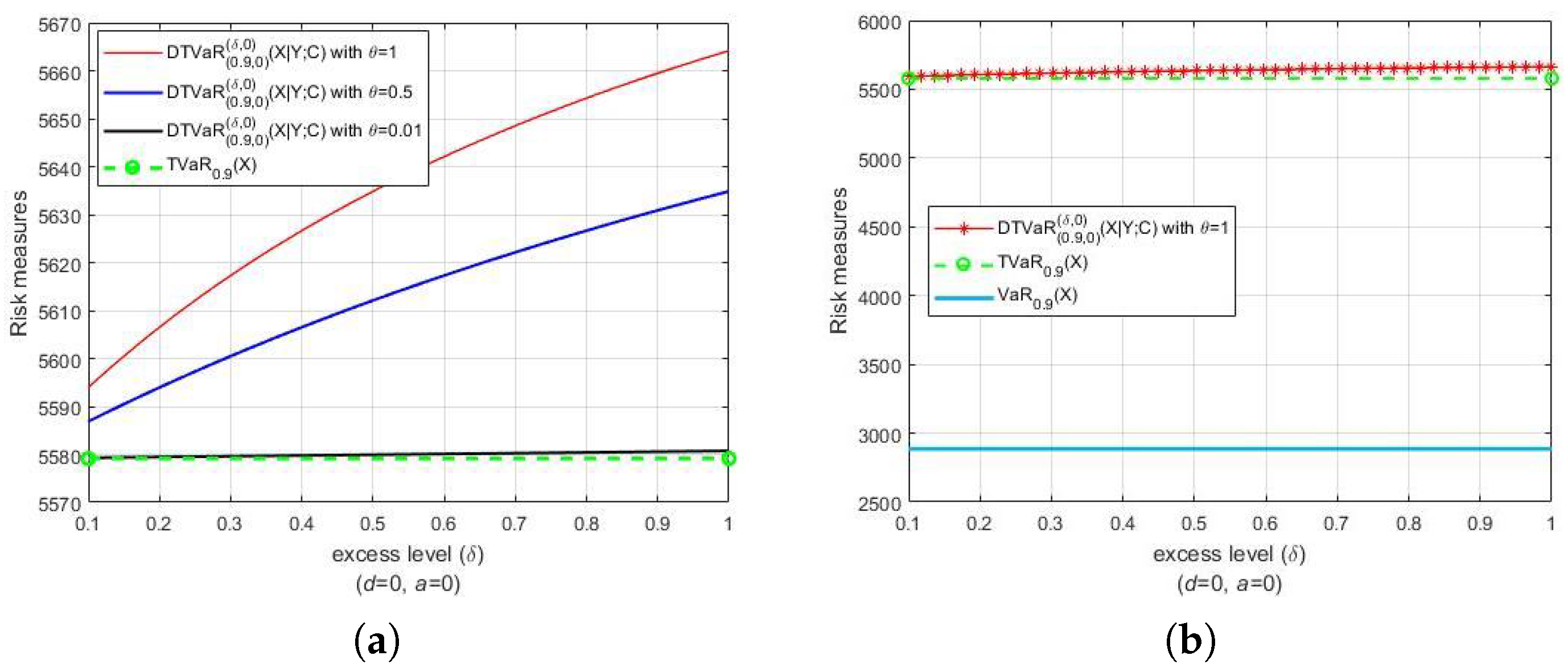
Figure 2.
(a) DTVaR of the target loss X with associated loss Y for negative values of FGM copula parameter and along with (b) its comparison with TVaR and VaR of X. Both X and Y are Pareto distributed ().
Figure 2.
(a) DTVaR of the target loss X with associated loss Y for negative values of FGM copula parameter and along with (b) its comparison with TVaR and VaR of X. Both X and Y are Pareto distributed ().
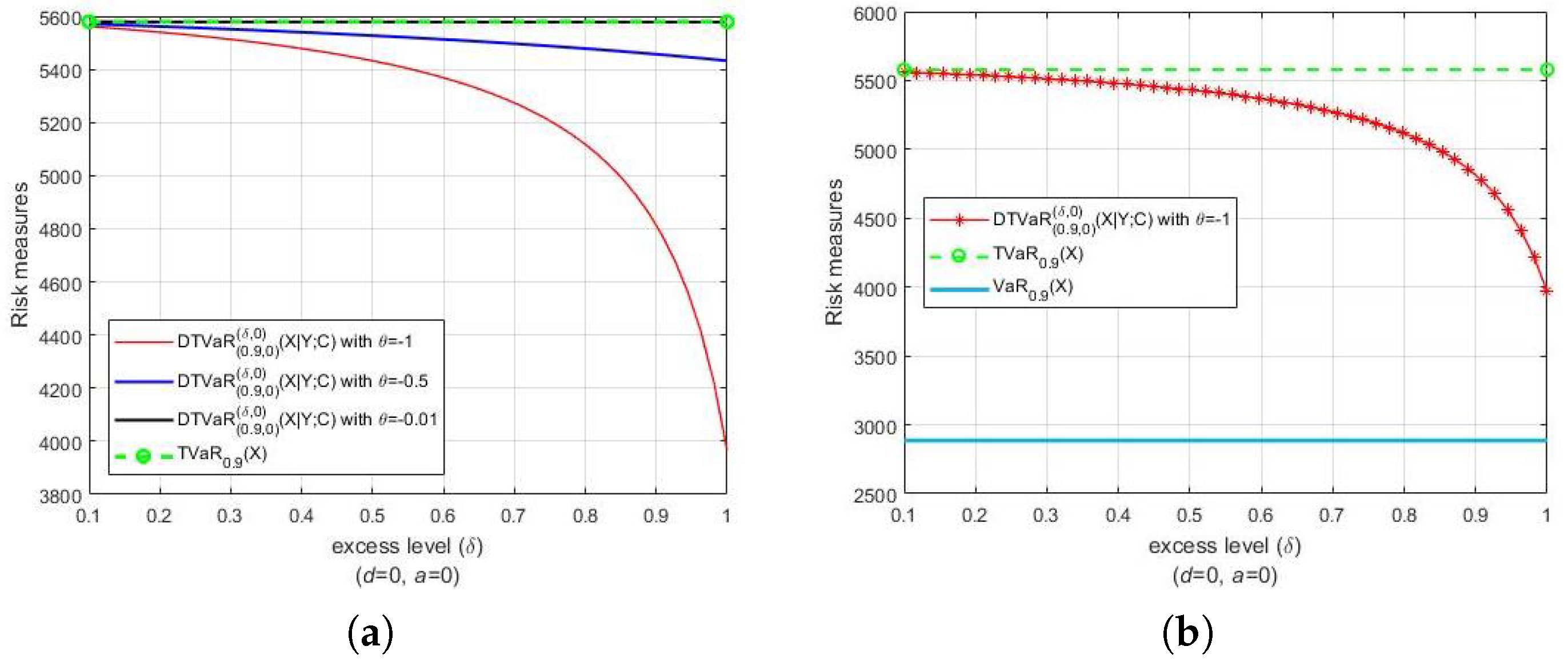
Figure 3.
(a) Histogram of insurance claim amount; (b) histogram of vehicle value; (c) box plot of insurance claim amount.
Figure 3.
(a) Histogram of insurance claim amount; (b) histogram of vehicle value; (c) box plot of insurance claim amount.

Figure 4.
DTVaR of the target loss X with associated loss Y and its comparison with (a) VaR of X and (b–c) TVaR of X. Both X and Y are Pareto distributed with , whilst FGM copula parameter estimate is
Figure 4.
DTVaR of the target loss X with associated loss Y and its comparison with (a) VaR of X and (b–c) TVaR of X. Both X and Y are Pareto distributed with , whilst FGM copula parameter estimate is
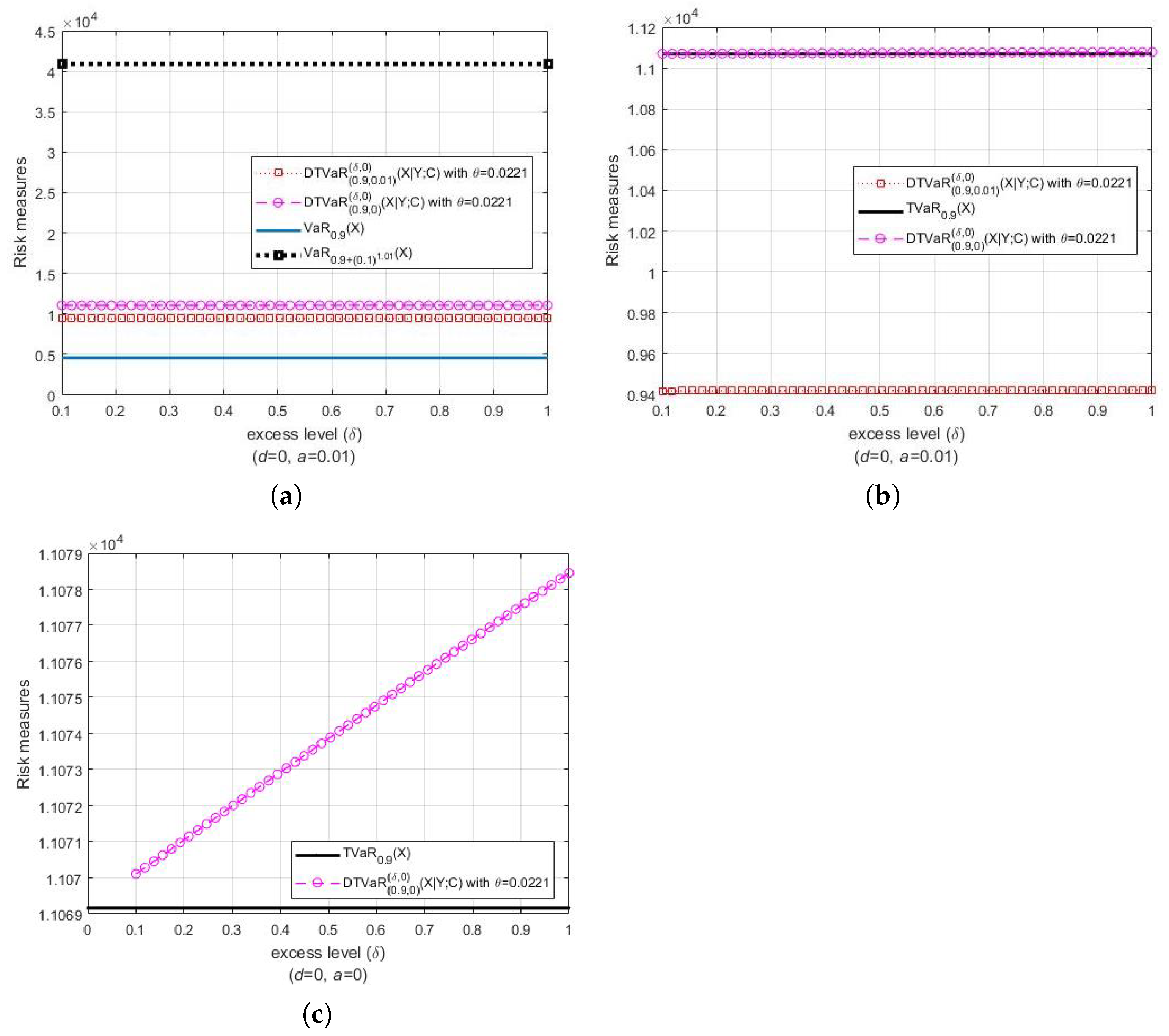
Figure 5.
The estimates of DTVaR of claim amount associated with vehicle value, along with the estimates of DTVaR and TVaR for (a) and (b) .
Figure 5.
The estimates of DTVaR of claim amount associated with vehicle value, along with the estimates of DTVaR and TVaR for (a) and (b) .
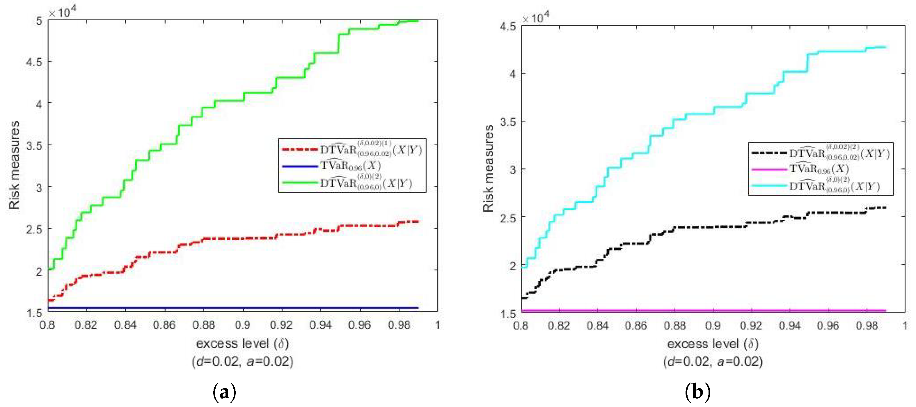
Figure 6.
(a) The estimates of DTVaR, , of claim value associated with vehicle value, along with their comparison with the estimates of DCTV for (b) and (c) .
Figure 6.
(a) The estimates of DTVaR, , of claim value associated with vehicle value, along with their comparison with the estimates of DCTV for (b) and (c) .

Figure 7.
Parametric estimates of DTVaR of claim amount associated with vehicle value, in comparison with nonparametric estimates for (a) and (b) .
Figure 7.
Parametric estimates of DTVaR of claim amount associated with vehicle value, in comparison with nonparametric estimates for (a) and (b) .

Table 1.
Descriptive statistics.
| Statistics | Claim Amount (X) | Vehicle Value (Y) |
|---|---|---|
| Sample number | 4618 | 4618 |
| Mean | 1.8616 | |
| Standard deviation | 1.1584 | |
| Skewness | 5.0470 | 1.8614 |
| Kurtosis | 43.3102 | 9.9344 |
Table 2.
Joint significance level and number of violations of nonparametric estimates of DTVaR and parametric estimates through FGM copula with .
Table 2.
Joint significance level and number of violations of nonparametric estimates of DTVaR and parametric estimates through FGM copula with .
| Method of Estimations | Estimators | 0.9 j.s.l. (%) | No. viol. (%) | Estimators | 0.92 j.s.l. (%) | No. viol. (%) | Estimators | 0.94 j.s.l. (%) | No. viol. (%) | Estimators | 0.96 j.s.l. (%) | No. viol. (%) |
|---|---|---|---|---|---|---|---|---|---|---|---|---|
| Nonparametric | DTVaR | 0.95 | 62 | DTVaR | 0.76 | 44 | DTVaR | 0.57 | 29 | DTVaR | 0.38 | 19 |
| (15,601) | (1.34) | (18,216) | (0.95) | (20,880) | (0.63) | (23,693) | (0.41) | |||||
| DTVaR | 65 | DTVaR | 49 | DTVaR | 33 | DTVaR | 20 | |||||
| (14,890) | (1.41) | (17,420) | (1.06) | (20,002) | (0.71) | (22,785) | (0.43) | |||||
| Parametric | ||||||||||||
| (Pareto, FGM Copula) | DTVaR | 130 | DTVaR | 103 | DTVaR | 65 | DTVaR | 41 | ||||
| (10,557) | (2.81) | (12,132) | (2.23) | (14,423) | (1.41) | (18,229) | (0.89) | |||||
| Nonparametric | DTVaR | 0.76 | 59 | DTVaR | 0.61 | 40 | DTVaR | 0.45 | 26 | DTVaR | 0.30 | 18 |
| (15,920) | (1.28) | (18,744) | (0.87) | (21,468) | (0.56) | (24,143) | (0.39) | |||||
| DTVaR | 65 | DTVaR | 47 | DTVaR | 33 | DTVaR | 20 | |||||
| (15,029) | (0.76) | (17,741) | (1.02) | (20,366) | (0.69) | (23,011) | (0.43) | |||||
| Parametric | ||||||||||||
| (Pareto, FGM Copula) | DTVaR | 130 | DTVaR | 103 | DTVaR | 65 | DTVaR | 41 | ||||
| (11,052) | (2.81) | (12,586) | (2.23) | (14,825) | (1.41) | (18,565) | (0.89) | |||||
| Nonparametric | DTVaR | 0.57 | 52 | DTVaR | 0.45 | 36 | DTVaR | 0.34 | 20 | DTVaR | 0.23 | 17 |
| (16,715) | (1.12) | (19,184) | (0.78) | (22,811) | (0.43) | (25,298) | (0.37) | |||||
| DTVaR | 63 | DTVaR | 47 | DTVaR | 27 | DTVaR | 18 | |||||
| (15,554) | (1.36) | (17,902) | (1.02) | (21,391) | (0.58) | (23,864) | (0.39) | |||||
| Parametric | ||||||||||||
| (Pareto, FGM Copula) | DTVaR | 130 | DTVaR | 103 | DTVaR | 65 | DTVaR | 41 | ||||
| (11,052) | (2.81) | (12,585) | (2.23) | (14,824) | (1.41) | (18,564) | (0.89) | |||||
| Nonparametric | DTVaR | 0.38 | 51 | DTVaR | 0.30 | 34 | DTVaR | 0.23 | 17 | DTVaR | 0.15 | 15 |
| (17,159) | (1.10) | (19,622) | (0.74) | (24,876) | (0.37) | (26,802) | (0.32) | |||||
| DTVaR | 63 | DTVaR | 47 | DTVaR | 20 | DTVaR | 18 | |||||
| (15,472) | (1.36) | (17,744) | (1.02) | (22,720) | (0.43) | (24,638) | (0.39) | |||||
| Parametric | ||||||||||||
| (Pareto, FGM Copula) | DTVaR | 130 | DTVaR | 103 | DTVaR | 65 | DTVaR | 41 | ||||
| (11,051) | (2.81) | (12,584) | (2.23) | (14,824) | (1.41) | (18,564) | (0.89) | |||||
| Nonparametric | DTVaR | 0.19 | 93 | DTVaR | 0.15 | 74 | DTVaR | 0.11 | 53 | DTVaR | 0.08 | 41 |
| (13,143) | (2.01) | (14,053) | (1.60) | (16,639) | (1.15) | (18,459) | (0.89) | |||||
| DTVaR | 92 | DTVaR | 74 | DTVaR | 52 | DTVaR | 40 | |||||
| (13,253) | (1.99) | (14,184) | (1.60) | (16,790) | (1.12) | (18,656) | (0.87) | |||||
| Parametric | ||||||||||||
| (Pareto, FGM Copula) | DTVaR | 130 | DTVaR | 103 | DTVaR | 65 | DTVaR | 41 | ||||
| (11,050) | (2.81) | (12,584) | (2.23) | (14,823) | (1.41) | (18,564) | (0.89) | |||||
1 No. viol. states the number of violations. 2 j.s.l. states the joint significance level expressed in percent. 3 The numbers in parentheses in columns 4, 6, 8, 10 and 12 indicate the percentages of violations to the data size (m = 4618).
Table 3.
DTVaR estimates and bootstrap confidence intervals.
| Estimators | ||||||
|---|---|---|---|---|---|---|
| DTVaR | 15,601 | 18,216 | 20,880 | 23,693 | 28,982 | |
| 12,826 | 13,189 | 13,233 | 13,057 | 11,630 | ||
| LCL | −0.3261 | −0.3585 | −0.3877 | −0.4408 | −0.5043 | |
| UCL | 0.3567 | 0.3937 | 0.4476 | 0.4860 | 0.5720 | |
| DTVaR | 14,890 | 17,420 | 20,002 | 22,785 | 28,059 | |
| 11,908 | 12,250 | 12,270 | 12,079 | 10,468 | ||
| LCL | −0.2784 | −0.3119 | −0.3598 | −0.4069 | −0.4719 | |
| UCL | 0.4462 | 0.4820 | 0.5410 | 0.5867 | 0.7214 | |
| DTVaR | 15,920 | 18,744 | 21,468 | 24,143 | 29,369 | |
| 13,366 | 13,789 | 13,841 | 13,672 | 12,346 | ||
| LCL | −0.3435 | −0.3869 | −0.4406 | −0.4784 | −0.5490 | |
| UCL | 0.3895 | 0.4422 | 0.4776 | 0.5228 | 0.6402 | |
| DTVaR | 15,029 | 17,741 | 20,366 | 23,011 | 28,218 | |
| 12,278 | 12,691 | 12,732 | 12,565 | 11,103 | ||
| LCL | −0.3017 | −0.3428 | −0.3844 | −0.4296 | −0.4988 | |
| UCL | 0.5095 | 0.5619 | 0.6233 | 0.6564 | 0.7848 | |
| DTVaR | 16,715 | 19,184 | 22,811 | 25,298 | 30,409 | |
| 14,148 | 14,530 | 14,567 | 14,291 | 12,954 | ||
| LCL | −0.3840 | −0.4233 | −0.4862 | −0.5222 | −0.6004 | |
| UCL | 0.4388 | 0.4971 | 0.5523 | 0.5970 | 0.6761 | |
| DTVaR | 15,554 | 17,902 | 21,391 | 23,864 | 28,987 | |
| 12,881 | 13,280 | 13,346 | 13,098 | 11,684 | ||
| LCL | −0.3358 | −0.3568 | −0.4303 | −0.4519 | −0.5566 | |
| UCL | 0.5700 | 0.6423 | 0.7151 | 0.7514 | 0.8861 | |
| DTVaR | 17,159 | 19,622 | 24,876 | 26,802 | 31,595 | |
| 15,074 | 15,541 | 15,540 | 15,205 | 13,923 | ||
| LCL | −0.4296 | −0.4775 | −0.5689 | −0.6046 | −0.6908 | |
| UCL | 0.5107 | 0.5495 | 0.6413 | 0.6918 | 0.8115 | |
| DTVaR | 15,472 | 17,744 | 22,720 | 24,638 | 29,412 | |
| 13,337 | 13,848 | 13,987 | 13,708 | 12,490 | ||
| LCL | −0.3640 | −0.4029 | −0.4832 | −0.5196 | −0.5904 | |
| UCL | 0.6988 | 0.7635 | 0.9066 | 0.9198 | 1.0359 | |
| DTVaR | 13,143 | 14,053 | 16,639 | 18,459 | 20,468 | |
| 6773.1 | 6644.3 | 5665.9 | 4318.5 | 1769.9 | ||
| LCL | −0.6585 | −0.6870 | −0.8201 | −0.9703 | −0.9887 | |
| UCL | 0.6671 | 0.6957 | 0.7464 | 0.7341 | 0.8679 | |
| DTVaR | 13,253 | 14,184 | 16,790 | 18,656 | 20,637 | |
| 6849.2 | 6,16.6 | 5715.9 | 4316.7 | 1711.9 | ||
| LCL | −0.6502 | −0.7013 | −0.8250 | −1.0162 | −1.1208 | |
| UCL | 0.6390 | 0.6518 | 0.7331 | 0.6889 | 0.7987 |
Table 4.
DTVaR estimates and bootstrap confidence intervals.
| Estimators | |||||||
|---|---|---|---|---|---|---|---|
| DTVaR | 15,910 | 19,014 | 22,145 | 25,388 | 30,139 | ||
| 13,783 | 14,325 | 14,403 | 14,114 | 12,694 | |||
| LCL | −0.3248 | −0.3862 | −0.4613 | −0.5435 | −0.5979 | ||
| UCL | 0.3840 | 0.4108 | 0.4380 | 0.4291 | 0.5628 | ||
| DTVaR | 14,939 | 17,907 | 20,928 | 24,151 | 28,936 | ||
| 12,657 | 13,207 | 13,297 | 13,033 | 11,482 | |||
| LCL | −0.2875 | −0.3471 | −0.4074 | −0.5003 | −0.5566 | ||
| UCL | 0.4912 | 0.5206 | 0.5557 | 0.5757 | 0.7132 | ||
| DTVaR | 16,242 | 19,801 | 22,439 | 26,026 | 31,517 | ||
| 14,197 | 14,767 | 14,829 | 14,509 | 12,651 | |||
| LCL | −0.3512 | −0.4359 | −0.4773 | −0.5801 | −0.6906 | ||
| UCL | 0.3453 | 0.3377 | 0.4072 | 0.3706 | 0.4660 | ||
| DTVaR | 15,189 | 18,594 | 21,139 | 24,711 | 30,312 | ||
| 13,049 | 13,649 | 13,739 | 13,474 | 11,457 | |||
| LCL | −0.2909 | −0.3844 | −0.4107 | −0.5234 | −0.6754 | ||
| UCL | 0.4593 | 0.4547 | 0.5226 | 0.5022 | 0.5964 | ||
| DTVaR | 17,580 | 20,330 | 26,482 | 28,849 | 31,595 | ||
| 15,440 | 15,908 | 15,573 | 14,912 | 13,923 | |||
| LCL | −0.4515 | −0.5125 | −0.6770 | −0.7624 | −0.6662 | ||
| UCL | 0.4726 | 0.4952 | 0.5424 | 0.5672 | 0.7846 | ||
| DTVaR | 15,801 | 18,342 | 24,243 | 26,648 | 29,412 | ||
| 13,712 | 14,252 | 14,113 | 13,507 | 12,490 | |||
| LCL | −0.3748 | −0.4290 | −0.5916 | −0.6701 | −0.5855 | ||
| UCL | 0.6643 | 0.7088 | 0.7794 | 0.8211 | 1.0668 | ||
| DTVaR | 17,308 | 20,218 | 27,083 | 29,875 | 33,249 | ||
| 15,909 | 16,553 | 16,419 | 15,676 | 14,387 | |||
| LCL | −0.4237 | −0.4849 | −0.6829 | −0.7833 | −0.7663 | ||
| UCL | 0.4719 | 0.4938 | 0.4801 | 0.4499 | 0.6182 | ||
| DTVaR | 15,375 | 18,031 | 24,598 | 27,461 | 30,994 | ||
| 14,097 | 14,846 | 15,054 | 14,430 | 13,158 | |||
| LCL | −0.3363 | −0.3979 | −0.5754 | −0.6828 | −0.6794 | ||
| UCL | 0.6686 | 0.7002 | 0.6862 | 0.6770 | 0.8527 | ||
Table 5.
DTVaR estimates and bootstrap confidence intervals.
| Estimators | |||||||||||
|---|---|---|---|---|---|---|---|---|---|---|---|
| DTVaR LCL UCL DTVaR LCL UCL | 12,500 6665.3 −0.0647 2.3908 12,595 6748.8 −0.0804 2.3226 | 12,500 6665.3 −0.0719 2.3684 12,595 6748.8 −0.0469 2.3294 | 11,406 6116.2 0.1294 2.7870 11,505 6223.1 0.1060 2.6779 | 18,301 4615.1 −0.1676 4.0913 18,476 4654.9 −0.1869 4.0551 | 18,301 4615.1 −0.1319 4.1357 18,476 4654.9 −0.1846 4.0480 | 18,301 4615.1 −0.1520 4.0711 18,476 4654.9 −0.1944 4.0487 | 20,468 1769.9 0.8529 12.3001 20,637 1711.9 0.8545 12.6727 | 20,468 1769.9 0.9921 12.6703 20,637 1711.9 0.7986 12.7271 | 20,468 1769.9 0.9070 12.5987 20,637 1711.9 0.7832 12.6842 | ||
| DTVaR LCL UCL DTVaR LCL UCL | 11,481 6243.5 0.1043 2.6871 11,576 6341.7 0.0759 2.6477 | 11,481 6243.5 0.1172 2.7063 11,576 6341.7 0.1068 2.6221 | 10,123 5222.3 0.3885 10,222 5362.1 0.3889 3.3928 | 17,459 4804.0 0.0013 4.1230 17,653 4867.9 −0.0120 4.0887 | 17,459 4804.0 −0.0240 4.1619 17,653 4867.9 −0.0516 4.0430 | 17,459 4804.0 −0.0054 4.1322 17,653 4867.9 −0.0019 4.0177 | 20,068 1880.4 10,297 118,503 20,264 1830.7 1.0705 12.2409 | 20,068 1880.4 1.1467 12.0218 20,264 1830.7 0.8565 12.0540 | 20,068 1880.4 1.1327 11.8399 20,264 1830.7 0.9883 12.0647 | ||
| DTVaR LCL UCL DTVaR LCL UCL | 11,481 6243.5 0.0971 2.6883 11,576 6341.7 0.1104 2.6320 | 11,481 6243.5 0.0969 2.7121 11,576 6341.7 0.1038 2.6449 | 10,123 5222.3 0.3918 3.4545 10,222 5362.1 0.3510 3.4162 | 17,459 4804.0 −0.0014 4.0688 17,653 4867.9 −0.0625 4.0382 | 17,459 4804.0 −0.0212 4.0664 17,653 4867.9 −0.0243 3.9866 | 17,459 4804.0 −0.0049 4.1201 17,653 4867.9 −0.0441 4.0767 | 20,068 1880.4 1.1327 11.8503 20,264 1830.7 0.9883 12.2752 | 20,068 1880.4 1.0817 11.8451 20,264 1830.7 0.9955 11.9624 | 20,068 1880.4 1.0736 11.8207 20,264 1830.7 1.0935 11.9624 | ||
| DTVaR LCL UCL DTVaR LCL UCL | 14,572 6950.0 −0.7380 0.5712 14,701 7030.0 −0.7490 0.5444 | 14,572 6950.0 −0.7253 0.5648 14,701 7030.0 −0.7425 0.5659 | 13,277 6679.9 −0.5678 0.8019 13,417 6790.9 −0.5666 0.7660 | 20,468 1769.9 −3.5026 0.6560 20,678 1687.6 −3.7977 0.5639 | 20,468 1769.9 −3.5026 0.6560 20,678 1687.6 −3.7977 0.5639 | 20,468 1769.9 −3.5026 0.6560 20,678 1687.6 −3.7977 0.5639 | 20,468 1769.9 −0.9887 0.8679 20,637 1711.9 −1.1208 0.7987 | 20,468 1769.9 −0.9887 0.8679 20,637 1711.9 −1.1208 0.7987 | 20,468 1769.9 −0.9887 0.8679 20,637 1711.9 −1.1208 0.7987 | ||
| DTVaR LCL UCL DTVaR LCL UCL | 14,572 6950.0 −0.7264 0.5789 14,701 7030.0 −0.7534 0.5714 | 14,572 6950.0 −0.7496 0.5870 14,701 7030.0 −0.7474 0.5659 | 13,277 6679.9 −0.5777 0.8008 13,417 6790.9 −0.5846 0.7533 | 20,468 1769.9 −3.5026 0.6560 20,678 1687.6 −3.7977 0.5639 | 20,468 1769.9 −3.5026 0.6560 20,678 1687.6 −3.7977 0.5639 | 20,468 1769.9 −3.5026 0.6560 20,678 1687.6 −3.7977 0.5639 | 20,468 1769.9 −0.9887 0.8679 20,637 1711.9 −1.1208 0.7987 | 20,468 1769.9 −0.9887 0.8679 20,637 1711.9 −1.1208 0.7987 | 20,468 1769.9 −0.9887 0.8679 20,637 1711.9 −1.1208 0.7987 | ||
| DTVaR LCL UCL DTVaR LCL UCL | 14,572 6950.0 −0.7504 0.5906 14,701 7030.0 −0.7474 0.5572 | 14,572 6950.0 −0.7370 0.6010 14,701 7030.0 −0.7294 0.5752 | 13,277 6679.9 −0.5672 0.8118 13,417 6790.9 −0.5914 0.7590 | 20,468 1769.9 −3.5026 0.5803 20,678 1687.6 −3.7977 0.5639 | 20,468 1769.9 −3.5026 0.6560 20,678 1687.6 −3.7977 0.5639 | 20,468 1769.9 −3.5026 0.6560 20,678 1687.6 −3.7977 0.5639 | 20,468 1769.9 −0.9887 0.8679 20,637 1711.9 −1.1208 0.7987 | 20,468 1769.9 −0.9887 0.8679 20,637 1711.9 −1.1208 0.7987 | 20,468 1769.9 −0.9887 0.8679 20,637 1711.9 −1.1208 0.7987 | ||
Publisher’s Note: MDPI stays neutral with regard to jurisdictional claims in published maps and institutional affiliations. |
© 2022 by the authors. Licensee MDPI, Basel, Switzerland. This article is an open access article distributed under the terms and conditions of the Creative Commons Attribution (CC BY) license (https://creativecommons.org/licenses/by/4.0/).
Share and Cite
MDPI and ACS Style
Syuhada, K.; Neswan, O.; Josaphat, B.P. Estimating Copula-Based Extension of Tail Value-at-Risk and Its Application in Insurance Claim. Risks 2022, 10, 113. https://doi.org/10.3390/risks10060113
AMA Style
Syuhada K, Neswan O, Josaphat BP. Estimating Copula-Based Extension of Tail Value-at-Risk and Its Application in Insurance Claim. Risks. 2022; 10(6):113. https://doi.org/10.3390/risks10060113
Chicago/Turabian StyleSyuhada, Khreshna, Oki Neswan, and Bony Parulian Josaphat. 2022. "Estimating Copula-Based Extension of Tail Value-at-Risk and Its Application in Insurance Claim" Risks 10, no. 6: 113. https://doi.org/10.3390/risks10060113
Note that from the first issue of 2016, this journal uses article numbers instead of page numbers. See further details here.