
A Hyperbolic Bid Stack Approach to Electricity Price Modelling

1
Finance Discipline Group, UTS Business School, University of Technology Sydney, Sydney, NSW 2007, Australia
2
School of Mathematical and Physical Sciences, University of Technology Sydney, Sydney, NSW 2007, Australia
3
The African Institute of Financial Markets and Risk Management (AIFMRM), University of Cape Town, Cape Town 7700, South Africa
4
Faculty of Science, Department of Statistics, University of Johannesburg, Johannesburg 2006, South Africa
*
Author to whom correspondence should be addressed.
Risks 2023, 11(8), 147; https://doi.org/10.3390/risks11080147
Submission received: 29 May 2023
/
Revised: 1 August 2023
/
Accepted: 2 August 2023
/
Published: 10 August 2023
Abstract
:Modelling the energy price in the Australian National Electricity Market (NEM) requires features that are not well reflected in existing models. We present a semi-structural, multi-regional model wherein bidding is not required to be cost-based, renewable fuels and storage technology are structurally integrated, and network constraints are often binding in optimal dispatch. Available fuel capacity then does not necessarily sum to registered bid capacity, as-bid fuel costs do not dependably follow input fuel prices, and cross-regional interconnectedness requires modelling trade. Furthermore, modelling the NEM spot price path must admit price negativity and price spikes. Extending previous work in the literature, the present paper proposes a hyperbolic bid stack approach to price modelling under these conditions.
Keywords:
electricity price modelling; bid stack functions; network constraint effects; structural price model; fundamental price modelJEL Classification:
C60; Q40; Q41; Q421. Introduction
1.1. Aims
Electricity price modelling is central to investment and asset valuation—including physical power investments, commercial licences, clean energy certificates, debt and equity claims, and financial derivatives—as projecting the cash flows of these types of assets usually requires the expected value of the electricity price. In addition, the optimal control and the financial risk management involved in using these types of assets are no less dependent on the electricity price evolution. These applications require a price model that recovers the common empirical features of the spot price path, including negativity and spikes, with distributional accuracy at the minimum.
There has also been a renewed interest in modelling the electricity price in such a way that the price effects of certain market factors such as the capacity changes of the regional fuel mix or the cross-regional interconnectors are traceable. These features open any price model to scenario analysis, commonly used in, e.g., commissioning and capacity planning, system constraint cost pricing, investigating interconnector arbitrage, setting regulatory price thresholds, etc., by the market operator and in regulatory oversight. Available capacity variation, replicating the ramping speed, must-run amounts, shut-down periods, etc., and the intricate link between intermittent generation and the price, as found in empirical studies by Maciejowska (2020); Paraschiv et al. (2014) and Mwampashi et al. (2021, 2022), have been sources of detailed modelling assumptions in recent years. These often also have a lot of data support, giving more accurate modelling frameworks that are often highly specific to the fuel mix (see for example Benth and Ibrahim 2017; Deschatre and Veraart 2017; Gianfreda and Bunn 2018; Moazeni et al. 2016). Models of this type, which aim to reflect the way prices are formed in market, are typically called “structural”, as opposed to “reduced–form” models which simply assume a particular stochastic dynamic for prices.
The objective of the present paper is formulating a semi-structural electricity price model that reflects the market design in Australia sufficiently well, while also recovering the most important empirical features of the price path and tracking the price effects of both the permanent and temporary capacity changes in the fuels and interconnectors. The proposed approach is, in this sense, structural. More precisely, we suggest a hyperbolic variation to the market merit order dynamics of Carmona et al. (2013), giving a bid stack model formulation that extends to renewable and storage power sources as well as to network restrictions in multi-regional settings.
1.2. Bid Stack Modelling Context
The bid stack model literature—starting with Barlow (2002), who retrieved the stochastic microeconomic market structure of Föllmer and Schweizer (1993) and wrote the spiky electricity price as a non-linear transformation of a jumpless diffusion process for demand—typically maintains a characteristic, fundamental set of assumptions about the pre-existing supply–demand and auction schema relations. Most bid stack models still at least implicitly retain this characteristic market structure with perfect demand inelasticity and friction (Carmona and Coulon 2014). Also, to obtain the price, the different parametric bid stack models give different forms to the aggregate supply function, i.e., the market bid stack function, as appropriate in the local context. These differentiations give various instances of the largely typical market structure. The rationale is that the price formation cannot significantly detach from the equilibrium mechanism as long as end-user demand is assumed inelastic and electricity is not economically storable. In what follows, we give a generic overview of wholesale price settlement from the Australian perspective, which, however, demonstrates that any strict non-storability assumption is already untenable at the operational level. Also, the market structure underpinning the usual bid stack framework can easily be adjusted for storability.
In Australia and in other countries, electricity is almost always cleared as a homogeneous commodity in an automated multi-unit and often also uniform price auction according to Krishna (2009). The wholesale price is typically determined from the participants’ bids, in a way that is based on economic principles under the physical constraints of the electric system, using constrained linear optimization programs, such as the NEM Dispatch Engine (AEMC 2020) in the Australian National Electricity Market (NEM). Simply put, this program collects the bids in the maximum registered capacity of the units, discards the ones that are physically infeasible (“constrained-off”), enforces those that cannot be omitted for feasibility reasons (“constrained-on”), and returns the least-cost price from the marginal prices at the optimum solution (AEMO 2022a).
Bids are a series of price–quantity pairs offered by a unit as terms of trade. There are two basic types of bids. Firstly, generator bids are placed by generator units of any fuel type—e.g., coal, gas, solar, battery, hydro, etc.—to sell electricity. Regardless of their availability, the units partition their full capacity into quantity blocks. They assign the lowest price that they would ask for producing every quantity block to each block. These are the price–quantity pairs, i.e., the generator bids. They submit as many bids as there are blocks, and that number is usually capped by the market operator. Secondly, load bids are placed by load units of any fuel type—e.g., battery, hydro—to buy electricity. Regardless of their availability, the units also partition their full capacity into quantity blocks. They then assign the highest price that they would offer for purchasing every quantity block to each block. These are the price–quantity pairs, i.e., the load bids. The units submit as many bids as there are blocks, and that number is usually capped by the market operator.
For market price settlement, the generator bids are pooled and arranged in ascending order on price, i.e., in merit order. The generator bid stack is the cumulative sum of the bid quantities in merit order, at or below every price on the complete set of bid prices in ascending order, from the regulatory price floor to the regulatory price cap. It is agnostic to the fuel type behind the bids. The generator bid stack is a left-continuous, step-wise relation that resembles the implied aggregate inverse supply. As such, the bid stack is typically plotted with the quantity on the horizontal axis and the price along the vertical axis. With fully inelastic end-user demand, the price at demand—where the vertical demand line intersects the generator bid stack—is the market price. It is the price of the last bid in merit, i.e., the price of the most expensive generator bid still needed to fill the demand in full.
Similarly, the load bids are pooled and arranged in descending order of price, i.e., in merit order. The load bid stack is the cumulative sum of the bid quantities in merit order, at or above every price on the complete set of bid prices in descending order from the regulatory price cap to the regulatory price floor. The load bid stack is a right-continuous, step-wise relation that resembles the implied inverse demand of the load units. Market price settlement is not complete without coalescing the load bid stacks with the generation bid stacks in the equilibrium mechanism. The load bids that are eventually granted uptake in addition to end-user demand are the ones at or above the market price. Consequently, in the presence of loading, aggregate demand is higher, and becomes slightly elastic, compared to the generation-only market structure.
Above, in stating that the bid stacks from the two basic bid types resemble implied inverse supply and implied inverse demand, respectively, we are assuming that there exist appropriate parametric formulae for transforming the bid information to supply and demand functions within a mostly typical stochastic market structure. For generator bids and the implied inverse supply curve, this is a fundamental assumption in the parametric bid stack model literature (Carmona and Coulon 2014). For load bids and the implied inverse demand curve, however, this is a new assumption.1
The more recent bid stack models that emulate the above mechanism make extensive and varied assumptions about what constitutes aggregate supply under the operational constraints of the electric system2, mostly through the capacity variation effect, which concerns the removal of unavailable capacity (Burger et al. 2004; Cartea and Villaplana 2008; Coulon et al. 2013) or similarly, the scarcity effect, which captures sudden capacity depletion (Aid et al. 2013; Howison and Coulon 2009), and the merit order dynamics, i.e., fuel bid curve aggregation, when the fuel types are differentiated (Aid et al. 2009, 2013; Carmona et al. 2013; Howison and Coulon 2009). The models propose different functional forms to the aggregate inverse supply function, but usually omit two-way (i.e., storage) fuels with loads. Also, some are more explicit about the underlying market structure than others (Filipović et al. 2018). The diversity of the literature on these models also shows that the geographic and commercial wholesale environment has a profound impact on the spot price trajectory.
Indeed, as wholesale electricity is traded almost immediately after it is produced, and always locally, the main features of the local market, such as the fuel mix, the network sparsity, and the rules and regulatory requisites of the automated auction algorithm, all tend to factor into price discovery to some extent (Eydeland and Wolyniec 2003). We argue that the properties of the local market routinely determine the correct modelling assumptions and heavily restrict the functional form of the aggregate supply function.
Somewhat surprisingly, the well-known bid stack models with fuel-type differentiation mentioned above all encounter difficulties at the model assumption level when simulating the NEM power price due to the following peculiarities of the local market: the already high and increasing renewable penetration, the ongoing two-way fuel expansion, the price effects of binding network constraints, the price-based auction mechanism, and the frequent price negativity as a result. At the same time, the seminal model by Carmona et al. (2013) has an attractive merit order dynamic, which the present work retrieves and adapts in five directions for an improved approach that better reflects the NEM.
In the NEM, the fuel mix is increasingly high in solar-, wind-, and hydropower (Department of the Industry and Resources 2020) and therefore the model cannot rely on the spot and futures prices of the input fuels, e.g., gas and coal, as closely as the existing literature suggests (Aid et al. 2013; Carmona and Coulon 2014; Carmona et al. 2013). Given, however, that the NEM has a price-based auction mechanism, i.e., that the participants can bid at any price within the regulatory price thresholds with no obligation to justify their price on a cost basis according to AEMC (2020), the proposed model can establish the fuel-specific bidding behaviours by fitting a time-dependent fuel bid stack function to the different fuel bid data with fuel-specific variables. Using the fuels, or explicitly evaluating the relationship between the bidding behaviour and the input fuel prices by fuel type, then recovers the implied inverse supply curves in reduced form without tying the fitted functions to the production costs or the utility equations of the individual plants (thus making the model “semi-structural” in this sense). In any liberalised market, this is applicable to all fuels in which the individual operators engage in bidding, including renewables.
While fitting the functions to the fuel bid data transfers easily between the different fuel types, the physically available capacity of the fuels cannot be readily captured by the same formulation. In the NEM, the individual participants bid in their full capacity (AEMC 2020); these are the bid data. They also provide other real-time technical data, e.g., ramp rates, renewable forecast measurements, etc., from which the available quantities can be ascertained centrally. Drawing on the same data set, rather than introducing a “hidden” variable for average capacity variation (Burger et al. 2004; Cartea and Villaplana 2008; Coulon et al. 2013) or a scarcity effect (Aid et al. 2013; Howison and Coulon 2009), the proposed model makes use of the technical data for approximating what constitutes the available aggregate capacity under the operational constraints.
The NEM also has a considerable amount of pumped hydropower and a rapidly growing battery fleet, as described in Department of the Industry and Resources (2020). These two-way fuels enter on both sides of the market by placing two distinct sets of generator and load bids, and thus open the typical market structure to demand elasticity with an evident effect on the electricity price. Therefore, the suggested equilibrium formulation that extends to two-way fuels is a new contribution in the bid stack modelling literature.
Furthermore, dispatch scheduling and price settlement in the NEM is subject to a myriad of security constraints. When some of these constraints bind, some bids are forced on (constrained-on) and others are curtailed (constrained-off) in result, depending on the constraint coefficients of the participating units placing the bids. It follows that the market bid stack, or more simply and equivalently (as we show) the demand quantity, must be adjusted to reflect these constraint effects on quantity. This is not a case of higher scarcity when the constrained-on quantities are considered, but a new feature we suggest incorporating into the usual market bid stack formulation.
Finally, the regulatory market price floor is AUD in the NEM and negative prices, incl. negative price spikes, are common. This requires a model that evaluates the positive and the negative price outcomes in much the same way. Although the existing bid stack models write elaborate mechanisms for positive prices, they only provide probabilistic overlays (Carmona and Coulon 2014; Carmona et al. 2013), if anything, for the negative prices. More commonly, they disallow (Filipović et al. 2018; Howison and Coulon 2009) or disregard (Aid et al. 2009, 2013) price negativity. In contrast, our approach assigns a hyperbolic form to the fuel bid stack functions and preconditions the negative price outcomes the same way as the positive ones, as long as the bid data record negative bids. This hyperbolic feature is akin to the spread adjustment method of Ward et al. (2019), who apply this to the short-term marginal cost of thermal technologies, in the sense that both approaches clearly identify what puts prices under downward pressure near the negative end of the price spectrum, and use a hyperbolic feature to reproduce it.
1.3. Other Structural Models
For completeness, it is worth mentioning further papers that model the electricity price as an equlibrium between supply and demand curves. Because they do this, these are all structural to some degree. However, the more refined (the more structural) a model, the more likely it is to reflect the settings of a specific exchange or wholesale market. A day-ahead market model in Europe might have very different ingrained assumptions, such as sequential arbitrage, stable offer capacity over time, lack of real-time balancing constraints, etc., compared to the requirements of a wholesale real-time market model for Australia. In addition, negative prices are relatively large and common in some regions in Australia, which is why the standard assumption of an exponential supply curve is not adequate in this setting without adjustments. Because of these, the applicability of the models below to the Australian market is limited.
The X-model proposed by Ziel and Steinert (2016) and further improved by Kulakov (2020) first creates a small number of price classes, i.e., price ranges that are sub-segments of the full price range. The authors then stochastically model the bid volume within every price class, whereby the correlation structure of the bids is also retained. Finally, the bid volumes are reassessed probabilistically for every discrete price within every price class. This is referred to as price curve reconstruction. The original model in Ziel and Steinert (2016) reconstructs both price curves for supply and demand, while Kulakov (2020) reworks the supply curve so that it contains the elastic negative supply bids from the demand curve, which allows for the demand curve to be perfectly inelastic. Therefore, Kulakov (2020) models the supply curve with multiple price classes, but only one price class for the demand curve. The name of the approach comes from the fact that in equilibrium the curves appear as the letter X. This approach would be problematic for Australia without first adjusting the bid-in data to the available capacity and constrained-on/off volumes (see Section 2.2.5 below). This is possible, but is not recommended by the authors. Moreover, the computational burden of the whole exercise would be much higher because more price classes would be required, since market prices might take any value on the range [AUD −1000, AUD 16,000] and not only [−EUR 50, EUR 3000].
Buzoianu et al. (2012) suggest an exponential supply curve function that incorporates temperature and seasonality effects, and distinguishes between gas-fuelled and non-gas generation. In addition, they formulate a linear demand function with an autoregressive component to equilibrate the two. Furthermore, Rassi and Kanamura (2023) use a stochastic power transform to map excess supply quantity minus LNG (liquefied natural gas) volume to the price using a closed-form expression. Their model takes a near-exponential shape for the supply curve when implemented on JEPX (Japan Electric Power Exchange) data. Neither of these models is likely to admit negative prices and they are most suitable for markets or price regions with a high share of natural gas.
Beran et al. (2019) assume a piece-wise linear supply curve, bidding at marginal cost by fuel type and a level of must-run CHP (combined heat and power) capacity. They apply fuel-specific available capacity truncation as well before obtaining the price at the intersection of supply and demand. This approach is well developed in terms of fuel specification, but the assumption that fuels are bid on at marginal cost is problematic for the Australian market. In Australia, disorderly bidding away from marginal cost and bid shading (submitting more than one price–quantity bid pair) are allowed.
Mahler et al. (2019) tackle the pricing problem as an optimisation, where the objective function minimises the sum of the parametrised marginal prices times residual generation quantities by production type. The authors make special adjustments for nuclear and hydroelectric plants. The parametric stack function for the marginal prices is linear. This model is also well developed in terms of fuel availability, but the linear assumption limits the model’s ability to predict positive and negative price spikes.
Pinhão et al. (2022) posit a polynomial form for the so-called price sensitivity curve, which is obtained by subtracting the supply curve from the demand curve. The root of this curve gives the price. The parameters of the curve are updated over time using a VAR model with harmonic components. This method does not attempt to isolate fuel-specific properties in the bid stack; therefore, similar to Ziel and Steinert (2016) and Kulakov (2020), one would need to adjust the fitted bid-in data for availability and constrained-on/off quantities first. Otherwise, the supply and demand curves cannot capture the true volumes after physical network constraints. These are, however, inevitably present in every real-time wholesale electricity market.
In summary, the current work is a hyperbolic variation of the market merit order mechanism put forward in Carmona et al. (2013). The new approach permits the inclusion of both renewable and two-way fuels, available capacities, and binding security constraints, and therefore better reflects the Australian wholesale environment in an interconnected regional setting than the existing models in the literature. Also, due to the hyperbolic formulation of the fuel bid stack functions, persistently observed price features, including negativity and spikes, arise semi-structurally in the model.
The paper is organised as follows. Section 2 gives the model formulation, with the main price map in Section 2.1 and the input processes in Section 2.2. Then, Section 4 presents some model implementation results for two different multi-regional demand specifications. Finally, Section 5 concludes.
2. New Approach
The proposed method captures supply and demand in the wholesale market to recover the electricity price as the equilibrium solution of the assumed market structure. The supply representation combines the supply from a multitude of power plants fuelled by a diverse range of generator fuels, e.g., coal, solar, hydro, etc., through time-dependent fuel bid stack functions. These express the supply contributed by each fuel over a range of price levels, as implied by the bid data of the plants using the fuel. Demand is a combination of end-user demand from the consumers, both industrial and household, in the region, export–imports, and demand from the load leg of the two-way fuels, e.g., pumped hydro and battery. End-user consumption plus trade (generation net of loads) is assumed perfectly inelastic and it is subject to a number of adjustments in the model. Formulating it as a diffusion process is generally sufficient for the model to admit a price sequence with spikes. In addition, we propose load fuel bid stack functions to capture the uptake demand of each two-way fuel over a range of price levels, usually with a degree of price elasticity, using the respective plant commitment (bid) data.
A market bid stack function is then built out of the fuel bid stack functions, noting that every fuel bid stack equation is fundamentally dependent on the typical availability variation in the particular fuel. This temporal variation can be linked to a factor that is physically induced, or to a factor that is both physically induced and arises out of the market mechanism. For example, the quantity of the solar supply relies on the rate of solar irradiance, an entirely physical component that puts an upper bound on the available quantity domain of the solar bid stack function. In contrast, the quantity of the coal supply usually relies on the ramp rates, a factor that is both physical and economic. The ramp-down rate poses a lower bound and the ramp-up rate an upper bound on the available quantity domain of the coal bid stack function. It is a physical factor, because the supply quantity range around the initial output level is based on the technical ramping specifications of the plants using the fuel. And it is an economic factor too, because the initial output level is the output quantity dictated by the equilibrium solution of the preceding time interval. In summary, the different fuel bid stack functions are defined on different quantity domains, as determined by the appropriate availability factors, prior to being aggregated in the market bid stack function.
The resulting market bid stack function is a time-dependent price map that transforms the expected value of the inelastic demand quantity into the expected value of the electricity price. Visually, the market bid stack function gives the price at the quantity where the inelastic demand, a vertical line, intersects the market supply curve, which is an increasing function over higher quantities. This is consistent with the merit order principles, as end-user demand is matched with least-cost supply first.
The quantities of the fuels generated and uptaken to meet end-user demand to realise the price result (dispatch quantities) are a consequence of the equilibrium solution, which highlights that compliance with the dispatch targets is what makes the scheduled units in a fuel compatible with the proposed framework. In the NEM, by use of the dispatch quantities at the end of the previous trade interval, the engine determines the optimal dispatch schedule and issues quantity targets based on it for the next interval (AEMO 2022a), i.e., the targets correspond to the dispatch quantities at the end of the current time interval provided that the plants change their dispatch precisely as prescribed. To orchestrate this, the engine has timely technical information about the physical limitations of the plants in all fuel types. Using that and other network data, it performs congestion and contingency planning to find the most optimal schedule for the period and to provide the plants with viable targets. In addition, for the purposes of a well-met congestion and contingency protocol, the market operator also enables ancillary response services (reserves) to maintain the operational frequency of the electric system between 49.85 and 50.15 Hz at all times (AEMO 2021). The ancillary balancing is necessary when the fuels are unable to change their dispatch quantities precisely as planned. However, the need for ancillary balancing never arises under the simplifying assumptions of the proposed hyperbolic price model. The available quantity domains of the fuel bid stack functions are presumed fully feasible, i.e., the fuels are modelled such that they are always able (and willing) to change their generation and uptake to any value within the available quantity domains of their bid stack functions. This is achieved by introducing fuel-level capacity limitations based on the unit-level available capacity limits as well as the constraint-driven capacity limitations that capture the network-wide infeasibilities of some quantities, e.g., for thermal overload, stability thresholds, tie-breaks, etc., subsumed under the constrained-on/off variable. These settings are designed to promote the accuracy of the available quantity domain in the model. Then, the fuels’ compliance, i.e., whether the units in the fuels in fact alter their dispatch as needed to realise the price result, is immediate under the model assumptions. Therefore, fuels that do not alter their generation and uptake at economic command cannot be modelled through fuel bid stack functions in the proposed approach.
Moreover, the units in the fuels may forgo bidding but still supply or demand smaller quantities. However, this only happens either when the plants are given a non-scheduled status at registration, or when they use fixed bids to act as price takers to secure trade with no price conditions. The model accommodates this activity using fixed bid quantity variables.
Then, perhaps the most important aspect of the equilibrium solution is the merit order dynamic. There are three steps involved in matching end-user demand with the least-cost supply, insofar as the availability and feasibility factors as well as the fixed bid quantities permit, that prepare our discussion of the merit order dynamic. The first step is to calculate the inelastic demand for the scheduled fuels to fill. For that, we take the net of the expected value of the inelastic demand term, the fixed bid quantities, and the constrained-on/off variable. The second step is to categorise the scheduled fuels as low-priced, mid-priced, or high-priced, for the following purpose. The low-priced generator fuels and the high-priced load fuels are granted complete dispatch and are netted against demand, just as, e.g., the fixed bid quantities are in step one. Then, the high-priced generator fuels and the low-priced load fuels with an available quantity lower bound at nil are taken out, i.e., their bids are removed from the merit order, as these quantities are uneconomic. If, however, the available quantity lower bound of a high-priced (uneconomic) generator fuel is not zero, i.e., the fuel is physically unable to shut down, then it is labelled an online fuel (a scheduled fuel that must be kept online). It remains dispatched in its lower-bound quantity and is netted from the demand at this time. There might be one or more online generator fuel simultaneously. That leaves the remaining mid-priced fuels as marginal to set the price at the adjusted inelastic demand, the demand for the marginal fuels to fill. The third step is to express the market bid stack function that returns the price at the adjusted inelastic demand in closed form.
The three steps in combination realise a market merit order dynamic that retains the core mathematical apparatus and the overlapping and dynamic properties of the Carmona et al. (2013) model, but also introduces three new price effects, which are the load effect, the online fuel effect, and the network constraint effect. The overlapping property allows the different bid stack functions to overlap on price. For example, solar may bid at prices between AUD −10 and AUD 10, coal between AUD 0 and AUD 100, and the fact that these overlap between AUD 0 and AUD 10 is perfectly acceptable. The dynamic property allows the fuel bid stack functions to be time-dependent, which is desirable for modelling the variability in the bid curves due to strategic bidding. The load effect is then the price effect that arises out of the two-way fuels entering with both a generator bid stack and a load bid stack at the same time. The online fuel effect ensures that fuels with a minimum operating level that cannot shut down are represented accordingly in the model. Lastly, the network constraint effect uses the constrained-on/off variable as a demand offset to avoid using quantities subject to curtailment but to use must-run quantities.
The regional market merit order dynamic that determines the dispatch quantities and the marginal price in the model is also subject to the influence of export–import between the regions in multi-regional markets. In real life, the dispatch engine of the NEM determines the price as the cost of the incremental 1 MW change in supply in the focus region by the end of the next 5 min trade interval, including the costs of the marginal energy targets and the consequential marginal frequency balancing target re-arrangements as per AEMO (2010), which involves interconnector availability as follows. When there is free interconnector capacity for price regions that have undispatched bids at lower prices, then the engine allows for trade and the regional prices are set at a similar level. In the absence of interconnector flow capabilities, however, the price is set within each focus region such that the prices of the different islanded regions are remarkably different. The model accommodates these export–import assumptions by carefully estimating the trade quantities between different regions within the respective interconnector capacity bounds that then enter as adjustments to the inelastic demand level.
The model generally maps well to other electricity markets that meet the following criteria. First and foremost, in regional markets the dual variables of the physical constraints should not be components of the marginal price. Also, the auction scheme of the market must be similar enough to that of the assumed market structure, i.e., to liberalised regional markets where the participants engage in price-based bidding. Whether bidding is price-based or cost-based in a market can impact the suitability of the model when capturing the price levels and the temporal changes in the fuel bid stack functions. The diurnal and seasonal shift variable of the proposed model is only concerned with strategic bidding, as is arguably appropriate in the price-based NEM; however, this may not be the recommended approach in cost-based markets, e.g., input fuel-price-based overlays might be needed for certain fuels. Moreover, sufficient historical non-price data must be available for the model to be accurately calibrated to ensure the physical feasibility of the projected equilibrium solutions over time.
Thus, the new approach returns the electricity price as the equilibrium solution of the assumed market structure as described. It is worth noting that the proposed hyperbolic model can also be helpful for the purposes of market analysis, as it does not detach from the production activity dictated by the auction scheme of the assumed market structure.
2.1. Model Formulation
The model works as a transformation map that takes inelastic demand as an input and produces price as an output at time t.
2.1.1. Fuel Bid Stack Functions
We denote with the scheduled generator fuel set of a price region, with the scheduled load fuel set of the same price region, and with the complete scheduled fuel set of the region. Let fuel be a generator fuel and fuel be a load fuel. We give two distinct fuel bid stack functions: one for the n generator fuels and another one for the m load fuels. Both have fuel-, region-, and time-dependent parameters. Additionally, we also introduce the price taker fuel set for the f fuels that make small, price-independent quantity commitments.
The time , which partitions the pricing period from time until time T into 5 min time intervals starting at .
At time t, the maximum registered capacity of generation fuel i is represented by , and the maximum registered capacity of load fuel l by , both measured in MW. Then, the maximum scheduled generation capacity of the region (in MW) is computed as the sum of the maximum scheduled registered generation capacities in the region, i.e., . The full capacity range of generation fuel i is and the full capacity range of load fuel l is . When proportionate to the maximum generation capacity of the region, the scaled full capacity range of generation fuel i is given by (in unit amounts), and the scaled full capacity range of load fuel l is given by (in unit amounts). The bid stack functions are fitted to data on these scaled full capacity ranges.
If the lower and upper availability generation bounds are and (in MW), respectively, then the available capacity range of generation fuel i would be . Similarly, if the lower and upper availability load bounds are and (in MW), then the available capacity range of load fuel l would be . When proportionate to the maximum generation capacity in the region , then the scaled available capacity range of generation fuel i would be (in unit amounts), and the scaled available capacity range of load fuel l would be (in unit amounts). The bid stack functions are restricted to these scaled available capacity ranges after the available capacity truncation.
Further, we introduce the regulatory price thresholds for the market price floor, which is usually negative (at around −$A1000), and for the market price cap (at around AUD 15,000 indexed to inflation) in AUD. When proportionate to the market price cap, at time t, the scaled price range between the regulatory thresholds would be or equivalently (in unit amounts).
Let the generator fuel bid stack function be the map from the scaled available capacity range of generation fuel i (the quantity x fuel i is able to trade) in unit amounts to the price range of generation fuel i (the price y fuel i receives per MW after scaling) in unit amounts as . While price y on the real codomain is a monotonically increasing function of quantity x, price y is not necessarily within the scaled regulatory thresholds. The economic interpretation of the map identifies it as an inverse supply curve, or as an implied inverse supply curve, when fitted to data.
Let the load fuel bid stack function be the map from the scaled available capacity range of load fuel l (the quantity x fuel l is able to trade) in unit amounts, to the price range of load fuel l (the price y fuel l pays per MW after scaling) in unit amounts as . While price y on the real codomain is a monotonically decreasing function of quantity x, price y is not necessarily within the scaled regulatory thresholds. The economic interpretation of the map identifies it as an inverse demand curve, or as an implied inverse demand curve, when fitted to data.
In this setting, we give two separate fuel bid stack functions, one for the generator fuels and another one for the load fuels.
First, we express the bid stack function for every generator fuel as a strictly increasing hyperbolic map from quantity in unit amounts to price in unit amounts, as
with at time t.
Then, for a left-continuous fuel bid stack map focusing only on the available capacity in the fuel, we define on the scaled available capacity quantity range of fuel i in most cases, except when the lower availability generation bound of the fuel is nil. In that circumstance, we define the map on .
Furthermore, we introduce the bid stack function for every load fuel as a strictly decreasing hyperbolic map from quantity in unit amounts to price in unit amounts, , as
with and at time t.
Then, for a right-continuous fuel bid stack map focusing only on the available capacity in the fuel, we define on the scaled available capacity quantity range of fuel l.
In comparison, Carmona et al. (2013) use exponential fuel bid stack functions on the positive real codomain for generation fuels only, making no assumptions about fuel availability.
Finally, the fuel bid curve equations for generator (1) and load fuels (2) are inherently symmetric. Before the availability truncation, the regional alpha captures the price elasticity (positive relationship) and the fuel beta the width (negative relationship) of the mid-range of the symmetric fuel curves. The regional alpha parameter is the same for all generator fuels i and load fuels l in the price region3. The beta parameter, i.e., for generator fuels and for load fuels, is specified for every fuel independently. However, the symmetry of the fuel bid stack equations is limited by the scope of the scaled full capacity range of generator fuel i on which its bid stack curve will have been fitted to the data , and also by the available capacity truncation.
2.1.2. Inverse Fuel Bid Stack Functions
We also propose inverse fuel curves, first in the spirit of Carmona et al. (2013) in general form, and then using the hyperbolic formulae to specify them.
Let the inverse fuel bid curve for fuel be the strictly increasing, left-continuous hyperbolic map from price y in unit amounts to quantity x on the scaled available capacity range, as4 , giving the lowest quantity x with at or above price y, if such exists, or giving the scaled available capacity upper bound otherwise as
as (see Carmona et al. 2013).
Analogously, let the inverse fuel bid stack function for fuel be the strictly decreasing, right-continuous hyperbolic map from price y in unit amounts to quantity x on the scaled available capacity range, as , giving the highest quantity x with at or above price y, if such exists, or else giving the scaled available capacity lower bound as
as .
2.1.3. Fuel Subset Definition
The fuel subsets help distinguish the type of quantity commitment made by each scheduled fuel within U. Two strands of quantity commitment are considered, constant and formulaic, for both generator and load fuels. Scheduled fuels are categorised as low-priced, mid-priced, or high-priced, and the type they are allotted determines the way they usually fill demand and set the price, i.e., they might enter as price-constant amounts or with price-dependent quantity formulae.
More specifically, every generator fuel can be completely dispatched (low-priced, constant), marginal (mid-priced, formulaic), online or unused (high-priced, constant). In contrast, the load fuels can be completely dispatched (high-priced, constant), marginal (mid-priced, formulaic), or unused (low-priced, constant), i.e., and are the only legal subsets loosely following Carmona et al. (2013).
Then, every generator fuel is allocated to one of the following four disjoint subsets, , as
Every load fuel is allocated to one of the following three disjoint subsets, , as
Furthermore, let be the market bid stack function that aggregates the fuel bid stack functions in formulaically, assuming that only the fuels in contribute formulaically to the market bid stack and that the fuels in the remaining subsets contribute to the demand quantity with price-constant quantity adjustments. From above, the set is the union of the marginal generator fuel set and the marginal load fuel set. Then, the function solves for the market price at the adjusted demand quantity x such that the value of the applied demand adjustment is linked to the subset specification .5 This adjusts demand by a term encapsulating the price-constant supply contribution of the fuels in , which gives . Thus, the value of x is not equal to , unless the supply contribution of the excluded fuels equals zero.
Denoting the upper price in generation fuel i at time t with and the lower price with , the merit order rule for generation gives that , i.e., the highest price in any completely dispatched generator fuel is always lower than the lowest price in any marginal generator fuel . Also, , i.e., the highest price in any marginal generator fuel is always lower than the lowest price in any online or unused generator fuel . Then, for n generator fuels on four subsets,6 the following fuel categorisation defines the elements of (low-priced), (mid-priced), and (high-priced):
- , generator fuel i is in subset . If the price from the market bid stack function 7 at quantity , the demand net of the quantity supplied by fuels , is greater than the highest price of any completely dispatched generator fuel ;
- , generator fuel i is in subset . If the price from the market bid stack function at quantity , the demand net of the quantity supplied by fuels , is lower than the lowest price of any online and unused fuel , , and if the lower capacity bound of fuel i is greater than 0;
- , generator fuel i is in subset . If the price from the market bid stack function at quantity , the demand net of the quantity supplied by fuels , is lower than the lowest price of any online or unused fuel , and if the lower capacity bound of fuel i equals 0;
- otherwise.
To explain these conditions for one fuel at a time, first consider a setting where the market price is already known. Given the upper and the lower price of fuel i, it can be assigned to a subset immediately by arranging and the market price in ascending order. If the market price is greater than , then is completely dispatched. Or, if the market price is lower than , then is online or unused, depending on the lower capacity bound . Otherwise, is marginal. But, because solves for the market price using the pre-existing subset allocation on , one cannot pinpoint the market price until are assigned to the correct subset, i.e., the market price is typically not yet known. One can, however, show that i always behaves online or unused on the price range , marginal on the price range , and completely dispatched on the price range from the given upper and the lower price of fuel i and the inverse bid stack formula in (3). By partitioning the entire price range at the upper and lower price of every fuel , one can obtain a string of smaller price segments8 and each segment then has a well-defined subset configuration associated with it, which is the same for all quantities within the segment, but may or may not be the same for two adjacent segments. The two price points defining each segment can be used to obtain the correct subset allocation by replacing “the market price” with the two price points and arranging and the two prices in ascending order. If the two price points are both greater than , then is completely dispatched. Conversely, if the two prices are both lower than , then is online or unused. Otherwise, is marginal.
Turning to the load fuels, let us denote the upper price of load fuel l with and the lower price with at time t. Using the merit order rules for load uptake, whereby , the lowest price for any completely dispatched load fuel is always greater than the highest price for any marginal load fuel , and the lowest price for any marginal load fuel is always greater than the highest price for any unused load fuel . The following are the fuel category conditions for m generator fuels on three subsets, (high-priced), (mid-priced), and (low-priced):
- generator fuel l is in subset . If the price from the market bid stack function at quantity , the demand net of the quantity supplied by fuels is lower than the lowest price for any completely dispatched load fuel ;
- generator fuel l is in subset . If the price from the market bid stack function at quantity , the demand net of the quantity supplied by fuels is greater than the lowest price of any unused load fuel .
- otherwise.
These conditions are perhaps more intuitive considering that a single fuel is always completely dispatched on the price range , marginal on the price range , and unused on the price range , as in the inverse bid stack formula in (5). By partitioning the entire price range at the upper , and the lower prices , of every fuel and , one obtains a string of smaller price segments, such that each segment has a particular subset configuration associated with it. The subset of fuel l can then be found using the above observation and the previously described subset process with this extended partitioning, as opposed to a more direct application of the subset rules.
In conclusion, the subsets of the fuels determine their role in filling the adjusted inelastic demand and consequently in price formation, i.e., in the market bid stack formula that solves for the market price. The completely dispatched fuels in are generated or uptaken in the quantity of their upper capacity bound or , which are constant in the sense that they do not depend on the exact price level beyond what is already known about the possible range of the price level that assigned them to in the first place. Similarly, the online fuels in are generated in the quantity at their lower capacity bound , which is also constant in that sense. Moreover, the unused fuels in are not generated or uptaken any quantity. In contrast, the marginal fuels in are generated or uptaken in some quantity within their capacity bounds, but the quantity has not been determined by the subset as such. Thus, from the perspective of the market bid stack formula , the type of quantity commitment the fuels must make due to being allocated to one particular subset and not to another polarises the subsets into constant dispatch and formulaic (marginal) dispatch subsets. The generation or uptake quantity of any fuel in the constant dispatch subsets is determined outside and enters as part of an additive term, i.e., as a demand adjustment, whereas the dispatch quantity of any fuel in the marginal dispatch subsets is determined by the market bid stack formula .
2.1.4. Market Bid Stack Formula
Let be the market bid stack function that aggregates every fuel bid curve on the complete regional fuel set under the appropriate subset allocation in merit order to evaluate the market price at quantity x. To that effect, first it distinguishes the constant dispatch fuels (in ) from the formulaic–marginal or price-setter fuels (in ).
The contribution of the former is captured in the constant term h that adds up the constant supply sum in the generator fuels with a negative sign and the constant demand sum in the load fuels with a positive sign as
To move these quantities to the inelastic demand side of the equilibrium, the demand quantity for the marginal fuels to fill can be expressed as .
In contrast, every marginal fuel in is represented by the inverse bid stack function of the fuel. The strictly increasing left-continuous market bid stack function maps the adjusted demand quantity to the highest price , such that the corresponding quantity over all inverse fuel bid stack functions is still below the cleared quantity , provided that there is at least one marginal generator fuel in the region. Then, the main structural components of the market bid stack, the constant term h and the aggregate of the inverse fuel curves, give the price solution of the function as
in general form, extending the market merit order dynamic of Carmona et al. (2013) (see Proposition 1 in Carmona et al. 2013) to a new generator fuel subset and to load fuels.
Then, the hyperbolic specification of (8) is expressed as
Example 1.
To demonstrate the proposed method, we consider a price region at time t with four generator and two load fuels, where the bid stack parameters and the adjusted inelastic demand quantity are already known, but remain unspecified. After careful arrangement9, the subset configuration is also already given. We know that of the generator fuels is completely dispatched, is online, and is marginal. Then, there is also completely dispatched and marginal load fuel.
We can then express h as
and denote the inverse fuel bid stack functions of the two marginal generator fuels with and , and the inverse fuel bid stack function of the marginal load fuel with .
2.1.5. Price Formula
The market bid stack function (9) solves for the market price under the normal market assumption. The value of demand implies the normal market assumption when it is between the lowest and the highest available generation quantity in the market. The values of and are specified shortly. The market price can then be written as . Conversely, should the market have either a demand deficit or a supply deficit , it is then in a system-tied state, and the corresponding prices are and , respectively. In general, we can express the market price as
i.e., the price in any state of the system.
To find the price in a normal market, let us partition the demand domain of the normal state into a string of quantity segments, such that one particular subset configuration holds for any level of demand within each segment. Finding the boundary points of the segments involves a corresponding string of price segments as well, as the quantity domain and the price codomain are bijective, since the fuel bid stack functions in (1) and (2) are strictly monotonic.
The boundary points of the price segments with the property can be given by the upper , and the lower , price points in all generation and load fuels in U. Let denote these prices in increasing order.
Then let, for every price , quantity be the quantity that sums the generation sum from the left-continuous inverse fuel maps in (3) with a positive sign, the uptake sum from the right-continuous inverse fuel maps in (5) with a negative sign, and the constant quantities h in (7) with a negative sign
giving the boundary points of the respective quantities also in increasing order.
Then, and . Additionally, every segment of the partitioned quantity domain , , , …, has a well-defined fuel subset combination associated with it that holds for any level of demand within the segment. The market bid stack function in (9) gives the price using the subset combination , which can be represented by for segment , by for segment , by for , and so on. For the same fuel set U, the appropriate fuel subset configuration changes over the different quantity segments. As a result, the market bid stack formula also has a segment-wise formulation, owing to its dependence on the segment-wise different .
Extending (10), we can then express price p as a segment-wise relation
where
loosely following Carmona et al. (2013).
Lastly, we recover the market price in AUD from the price in (12). To obtain , the price in unit amounts is multiplied by the market price cap and the result is projected to the regulatory price floor or cap , if it is exceeding either of the two. The reason why the threshold restriction has been delayed until now is that tracing the fuel dispatch quantities over time, i.e., computing the generation and the uptake quantities from the inverse fuel curves based on , requires strictly monotonic fuel bid stack formulations, which an untimely threshold projection could potentially impair.
Example 2.
We suggest an efficient algorithm for finding the appropriate fuel subset configurations on all segments of the partitioned demand domain and executing pricing using (12). To see how this computation works, we consider a price region with five generator and two load fuels, where the bid stack parameters and the demand quantity are already known. The scaled available capacity ranges and and the fixed net generation quantity (if any) are also already specified at the start of the algorithm as shown in Table 1.
Table 1 shows the four scheduled generator fuels (G1–G4), the one price taker generator fuel (G5), and the two scheduled load fuels (L1–L2) in this example. First by fuel type, which identifies the fuel source and places the six scheduled fuels in set and the one price taker fuel in set F. It then gives the bid stack parameters of the fuels. In the third column, the table specifies the available capacity ranges of the fuels in MW, which is subsequently scaled by the maximum registered generation capacity , which appears to coincide with the total available (scheduled) generation capacity in the region. We also have the lowest available generation capacity in the region as 10. The fourth column shows the price ranges of the fuels, which have been calculated using the bid stack parameters, the quantity ranges, and the maximum registered generation capacity. Finally, it is also stated that the region has a regulatory market price floor of and a cap of .

Table 2.
Market view.
| Price | −$5 | −$4 | −$3 | −$2 | −$1 | $0 | $1 | $2 | $3 | $4 | $5 | $6 | $7 | $8 | $9 | $10 | $11 | $12 | $13 | $14 | $15 |
|---|---|---|---|---|---|---|---|---|---|---|---|---|---|---|---|---|---|---|---|---|---|
| Generation quantity | |||||||||||||||||||||
| G1 | 30 | 30 | 30 | 30 | 30 | 30 | 91 | 100 | 105 | 109 | 111 | 114 | 116 | 117 | 119 | 120 | 120 | 120 | 120 | 120 | 120 |
| G2 | 0 | 0 | 0 | 0 | 0 | 0 | 16 | 19 | 20 | 21 | 22 | 22 | 23 | 23 | 23 | 24 | 24 | 24 | 25 | 25 | 25 |
| G3 | 0 | 0 | 0 | 1 | 2 | 7 | 7 | 7 | 7 | 7 | 7 | 7 | 7 | 7 | 7 | 7 | 7 | 7 | 7 | 7 | 7 |
| G4 | 0 | 0 | 0 | 0 | 0 | 0 | 0 | 0 | 1 | 1 | 1 | 1 | 2 | 2 | 2 | 2 | 2 | 2 | 2 | 2 | 3 |
| Total | 30 | 30 | 30 | 31 | 32 | 37 | 114 | 126 | 132 | 137 | 141 | 144 | 147 | 149 | 151 | 153 | 153 | 154 | 154 | 154 | 155 |
| Load uptake quantity | |||||||||||||||||||||
| L1 | 20 | 20 | 19 | 18 | 16 | 0 | 0 | 0 | 0 | 0 | 0 | 0 | 0 | 0 | 0 | 0 | 0 | 0 | 0 | 0 | 0 |
| L2 | 25 | 25 | 25 | 25 | 24 | 14 | 4 | 3 | 2 | 1 | 1 | 0 | 0 | 0 | 0 | 0 | 0 | 0 | 0 | 0 | 0 |
| Total | 45 | 45 | 44 | 43 | 39 | 14 | 4 | 3 | 2 | 1 | 1 | 0 | 0 | 0 | 0 | 0 | 0 | 0 | 0 | 0 | 0 |
| Net market quantity (generation minus load uptake) | |||||||||||||||||||||
| Total | −15 | −15 | −13 | −12 | −7 | 23 | 110 | 123 | 130 | 136 | 140 | 144 | 147 | 149 | 151 | 153 | 153 | 154 | 154 | 154 | 155 |
The table gives a tabulated view of the market showing the contribution of each scheduled fuel to the net market quantity (bottom line) at any price level. As the price increases, the generator fuels are contributing more and the load fuels are demanding less. For a more concise view, the price range (in AUD) has been discretised to integers and the quantity amounts (in MW) have been rounded to integers as well. The quantities shown in bold are obtained from the inverse fuel bid stack functions (4) and (6). The remaining (not bold) quantities are constants, as these are either below the available quantity lower bound or above the available quantity upper bound in the given fuel as per Table 1.
Then, Table 2 carries the main operations of the algorithm, which are the following:
- 1.
- Obtain the lower and the upper available capacity bound quantities from the third column in Table 1, i.e., every and in MW. Scale (divide) these by the maximum registered generation capacity . Then, use the fuel bid stack functions in (1) and (2) to find the corresponding prices, i.e., the upper , and the lower , price points, as shown in column four in Table 1, e.g., AUD 0 and AUD 10 for G1, AUD 0 and AUD 14 for G2, etc. When scaled by AUD 14 and in increasing order, these prices correspond to . For exposition purposes, Table 2 (unscaled view) also fills the price interval with additional prices for an evenly spaced price interval between −AUD 5 and AUD 15 (first row). Also notice that the prices are not yet projected to the regulatory price thresholds −AUD 4 and AUD 14.
- 2.
- Fill the table with the constant quantities (not bold) at the prices outside the price ranges of the fuels, i.e., with and . See lines G1, G2, G3, G4 and L1, L2 in Table 2. Notice how the G1 line lists 30 MW at every price level up to AUD 0. This way, if the market price ends up below price AUD 0 (and G1 is online in ), it would still be accounted for and dispatched in 30 MW.
- 3.
- 4.
- Sum the quantities in rows G1, G2, G3, G4 vertically at every price for the generation quantity total. Similarly, sum the quantities in the L1, L2 lines for the load uptake quantity total. Take away the load uptake total from the generation total to obtain the net market total at every price (last row), which is equivalent to the interval plus h (unscaled view in Table 2).
- 5.
- Assume the constrained-on/off adjustment (in MW). Obtain the inelastic end-user demand proxied by net generation (in MW), the fixed net generation quantity of the price taker fuels 1.5 MW (see Table 1), and the maximum generation 155 MW in the region. Then, the adjusted inelastic demand is computed as . We are going to look at two different demand levels. Firstly, when 31 MW. Secondly, when 115 MW.
- 6.
- Establish the state of the market, i.e., whether holds. From earlier, and . Thereby, the market has a demand deficit at and it is in a normal state at .
- 7.
- If the market has a demand deficit, every scheduled fuel is or and the price (in unit amounts) is set by , which then may be multiplied by and projected to the regulatory thresholds to obtain the market price in AUD—this is the end of the algorithm.
- 8.
- In a normal market, obtain the two quantity points (last row) nearest to and obtain the corresponding two price points too (first row). We have that falls within 110 and 123 (last row), and price AUD 1 and AUD 2. Using the two prices, we can assign every fuel to a subset using simple rules.
- 9.
- For generator fuels G1, G2, G3, G4, if the two prices AUD 1 and AUD 2 are both greater than , then fuel is completely dispatched. Or, if the two prices are both lower than , then fuel is online or unused. Otherwise, fuel is marginal.
- 10.
- For load fuels L1, L2, if the two prices AUD 1 and AUD 2 are both lower than , then fuel is completely dispatched. Or, if the two prices are both greater than , then fuel is unused. Otherwise, fuel is marginal.
- 11.
- Obtain the price (in unit amounts) from the market bid stack functionin (9) using the subset configuration on from above. Back out the current dispatch quantity in each fuel. Then, may be multiplied by and projected to the regulatory thresholds to obtain the market price in AUD—this is the end of the algorithm.
2.2. Input Processes
The market price Formula (12) requires several input processes including the formulaic bid stack function parameter that captures strategic bidding over time, the fuel-specific processes of available capacity truncation, the fixed capacity input, the constrained-on/off quantity process that encompasses network feasibility, and finally also the pre-adjustment demand term, which we decompose into regional consumption and export–import.
2.2.1. Fuel Gamma
The formulaic fuel gamma , i.e., for generator fuels and for load fuels, expresses what proportion of the maximum fuel capacity is being offered at negative prices for a given fuel at time t. More precisely, is the inflection point of the fuel bid curve (1) for generator fuel i and is the inflection point of the formulaic load bid stack (2) for load fuel l. The fact that these are time-dependent assumes that bidding activity changes over time, i.e., the bid stack functions shift horizontally as gamma changes over time.
For any time in the pricing period, we can give the day and the time can be identified precisely. Let be the day of year, assuming leap years. Then, we denote with the time of year for time points per day, i.e., is the time of day. For example, for , has 5 min increments. Further, let be a shifted time-of-day parameter
Further, is a sinusoidal function that captures both yearly seasonality for the day of year through parameters and diurnal variation for the time of day using .
For a generator fuel i, we express as
For a load fuel l, we give as
Note that the gamma parameters of the fuel bid curves can take the formulaic form directly from (14) and (15) at time t.
An alternative to this would be estimating the initial gamma parameters together with the initial alpha and beta parameters of the fuel bid curves using the least-squares method. Then, over time, by updating the gamma parameter by the cyclical change in the formulaic form, while retaining its estimated level from , we would have
2.2.2. Available Capacity
Available capacity truncation involves restricting in (1) for generator fuel i to quantity x on to the scaled available capacity range in unit amounts. Also, we let in (2) for load fuel l take a quantity x on the scaled available capacity range in unit amounts for all fuels.
From a non-stop power system point of view, the available capacity range is the range around the initial dispatch quantity at time that bounds the dispatch quantity at time .
A non-zero lower capacity bound is necessary whenever a fuel, i.e., the individual plants in a fuel collectively, is unable to shut down immediately. Regardless of the economic value of their activity, the units in this position are usually given appropriate non-zero targets in the central dispatch optimisation (AEMO 2010). In the model, we have an analogous treatment for the fuels with inflexible ramping profiles and minimum loading requirements, e.g., black and brown coal, in anticipation of this problem, using non-zero lower capacity bounds and the online fuel category .
In addition, different upper bounds arise as the availability up to the maximum registered capacity rarely holds in most fuels. First, given the ramp rate specifications and the length of the scheduling intervals, the units in the fuel might be too slow to ramp up to a higher, economically feasible capacity region, approaching the maximum registered fuel capacity at time by the start of next interval at . Second, the units of particular fuels are often unwilling or unable to be produced at their full capacity due to external factors, such as existing ancillary commitments, planned outages, or, more commonly, weather effects. Third, there are two-way fuels that trade both sides of the market, i.e., act as generators or loads interchangeably over time. As any load unit, e.g., pumped hydro or battery, would need to charge up in order to “produce” electricity, load units are usually registered in both categories and bid on in both categories as well to participate accordingly (AEMC 2020). In this sense, we refer to them as two-way fuels. Two-way fuels are actively balancing a storage level, which usually determines their remaining capacity for load uptake and generator dispatch at the same time.
Moreover, the model can capture the permanent changes in the maximum registered fuel capacity of the regional fuel mix for some time ahead, e.g., at the anticipated commissioning or decommissioning of units. The available capacity truncation is then a subsequent layer of capacity reduction.
Let be the dispatch quantity in generator fuel i and be the dispatch quantity in load fuel l, at time , in unit amounts. After we have the market price at time from (12), we can obtain the current dispatch quantity of a fuel by passing in the inverse fuel bid stack function of the fuel in (4) for a generator fuel i and in (6) for a load fuel l. We then give the available capacity bounds and at time around the dispatch level at the end of the previous time interval in a fuel-specific manner.
Base Case
Let , denote the ramp-up and ramp-down rates in MW/5 min for every generator fuel i and , the ramp-up and ramp-down rates in MW/5 min for every load fuel l. Furthermore, let m denote the regional ramp rate multiplier. This multiplier makes an allowance for the distortions arising out of the fact that the unit ramp rates are aggregated at fuel level to obtain the fuel-level ramp rates instead of applying unit-level ramping directly.
Across all fuels, particularly fossil fuels, e.g., coal, gas, etc., as a base case solution we can specify the available capacity bounds in MW using these fuel-specific ramp-up and ramp-down rates as follows. Let the lower availability bound of fuel i or l at time be the higher value of the dispatch quantity in the previous period minus the ramp-down rate and 0 as
Then let the upper availability bound of fuel i or l at time be the lower value of the dispatch quantity in the previous period plus the ramp-up rate and full as-bid fuel capacity
Assuming that the ramp rate specifications are time- and dispatch-level-invariant, we write these as averages and estimate them from the historical ramp rate data for the different fuels, ensuring that the MW/minutes raw ramp rate data are interpreted correctly11.
Intermittent Fuels
Across renewable fuels, such as solar and wind, as an intermittent case solution, we can give the available capacity upper bounds in MW using fuel-specific available capacity forecasts. This assumes either the direct or the indirect availability of some renewable generation forecast measures via prediction models or predictive indicators. We opt for two very simple forecast processes for the upper availability bounds of solar and wind generation.
Let the lower availability bound of intermittent fuel i at time be zero . This is a reasonable approximation as the ramp-down rates are generally quite high and not restrictive in renewable generation.
Let the upper availability bound of solar energy i at time t be estimated by a deterministic sinusoidal intraday generation function specified as
where is the time of day for observations per day. In this formula, the sum of two shifted sine functions is evaluated for generation between 0 and an upper bound g.
Finally, let the upper availability bound of wind generation at time t be estimated by a scaled Brownian motion discretised as
such that , where we denote with the time increment and with and the allowed thresholds of wind output.
Two-Way Fuels
Two-way fuels, such as hydro plants and batteries, actively balance a storage level k over time. Generator dispatch is at time t and the remaining capacity for load uptake is times the maximum capacity in the fuel .
An interesting outcome of the proposed hyperbolic market bid stack method is that the implied storage level k can be inferred from the modelled dispatch solution at the end of each interval when leaving the storage level unrestricted at the beginning of the interval.
Minimum Capacity Criterion
Fuels that are slow to start up often have operational capacity minima in the price settlement and scheduling process of the market operator, i.e., minimum load amounts. We represent this in the model for all affected generator fuel i via the lower-bound criterion in unit amounts, such that the available capacity lower bound of the fuel is always at or above this criterion .12
2.2.3. Net Fixed Generation by Price Takers
Apart from the basic bid types used in compulsory bidding, fixed bids are optional for both generators and loads in the NEM (AEMC 2020). In a fixed bid, the bidder opts to trade a predetermined amount at the regional market price as price taker. At time , we denote the fixed bid quantity in generator fuel with and the fixed bid quantity in load fuel , both measured in MW.
We also introduce for the net non-scheduled generation quantity in the region (in MW) at time to capture the quantity flows of the small-scale units excluded from bidding (AEMC 2020).
Then, we express the fixed net generation quantity as
at time .
The price taker quantities enter the pricing mechanism in two ways. First, the fixed net generation quantity (in MW) needs to be subtracted from the end-user demand as an adjustment when we calculate the demand for the scheduled fuels to fill.
Second, if a generator fuel i or load fuel l has both a bid stack function and a non-zero fixed bid quantity at time , i.e., or , respectively, then the time dispatch quantity of that fuel would have to be revised accordingly. In case of a generator fuel i that is both a scheduled and a price taker at the same time , the fixed bid quantity would have to be added to the dispatch quantity at the end of the time interval for . Similarly, in such a load fuel , the fixed bid quantity would have to be added to the dispatch quantity for . In principle, this can impact the available capacity bounds of the particular fuel at time .
2.2.4. Demand
The demand term incorporates trade as follows. Let represent the input process for net regional generation, the maximum scheduled generation, the fixed net generation of the price taker fuels, and the input process for the net constrained-on/off quantity in the price region at time t. The quantity can then be computed as in unit amounts, where can be expressed as a deterministic function with yearly seasonality for the day of year through parameters and diurnal variation for the time of day using
and is from (21) and is introduced in Section 2.2.5.
2.2.5. Constrained-On/Off Quantity
In practice, price settlement is performed by a linear programming (LP) engine subject to thousands of security constraints. Often, the binding constraints force the dispatch of some bid quantities and prevent the dispatch of some others. These are referred to as constrained-on and constrained-off quantities, respectively.
Let denote the constrained-on (must-run) generator quantity sum in the region. This is the quantity extent to which the generators are dispatched in the bids offered at prices above the realised market price, i.e., the generators in the region collectively receive higher targets by than what is expected on a price basis. When parsing the supply data in merit order, we want to take into account the effect of using these expensive bids, which can be achieved by reducing end-user demand by . Note that this term refers to all must-run generator quantities in the system, which is broader than the ramp-rate-implied must-run quantity over all fuels in set . More specifically, .
Let denote the constrained-off (curtailed) generator quantity sum in the region. This is the quantity extent to which the generators are not fully dispatched in the bids offered at prices below the realised market price, i.e., the generators in the region collectively receive lower targets from that what is expected on a price basis. When parsing the supply data in merit order, we want to skip over these unused inexpensive bids, which can be achieved by incrementing end-user demand with .
Let denote the constrained-on (must-run) load quantity sum in the region. This is the quantity extent to which the loads are dispatched in the bids offered at prices below the realised market price, i.e., the loads in the region collectively receive higher targets from than what is expected on a price basis. When parsing the supply data in merit order, we want to take into account the effect of exceedingly high targets for the price, which can be achieved by incrementing end-user demand with .
Let denote the constrained-off (curtailed) load quantity sum in the region. This is the quantity extent to which the loads are not fully dispatched in the bids offered at prices above the realised market price, i.e., the loads in the region collectively receive lower targets from than what is expected on a price basis. When parsing the supply data in merit order, we want to skip over these missed expensive load bids, which can be achieved by reducing end-user demand with .
It follows that the constrained-on/off quantity is the sum of the above introduced variables
which is expressed stochastically as
and is subtracted from demand before adjustments.
3. Model Implementation
The implementation of the proposed approach is now described. The results are from three 31-day periods between 4:00 A.M. 1 January 2022 and T 4:00 A.M. 1 February 2022, 4:00 A.M. 1 May 2022 and T 4:00 A.M. 1 June 2022, and 4:00 A.M. 1 October 2022 and T 4:00 A.M. 1 November 2022 for 5 min time intervals (8928 observations each period).
For both model variations A and B, the implementation begins by obtaining the fuels on the regional fuel set U in full capacity 13, and initialising the ramp rates , and the fixed bid quantities . The hyperbolic fuel bid stack formulae are then fitted to the stacked fuel bid data to acquire the fuel bid curve parameters at time .
The time-dependent input processes are initialised for . First, strategic bidding is captured by altering the value of the intercept variable of every fuel bid curve , i.e., by shifting the bid curves over time. Moreover, available capacity truncation is executed to restrict the fuel bid stack functions to their available capacity quantity domains defined between a lower and an upper capacity threshold for each trading interval. The upper capacity bounds of the renewable fuels follow formulaic relations and ramp rates are applied around the initial dispatch quantity in other fuels to obtain both the lower and the upper bounds. Furthermore, the physical feasibility of the fuels overall under the binding network constraints is also time-dependent. This enters the model via the constrained-on/off variable , which adjusts demand over time. Then, demand given as generation is also updated using the applicable time-dependent formulae.
The fuel set allocation and price calculation are performed as in Section 2, noting that because the wind availability and the constrained-on/off variable are stochastic, one must also iterate the model a number of times for every time point. The current implementation takes 25 iterations before averaging those for the model result.
3.1. Data Source
3.2. Fuel Summary
All plants present within the Bidmove Complete file (AEMO 2023b) with a dispatchable unit identifier (DUID) at time 14 are mapped to fuel types using the market operator’s mapping in AEMO (2022b) to retrieve the regional fuel sets. Each fuel type with a non-zero full bid capacity is included15 as shown in Table 5, Table 6 and Table 7.
3.3. Fuel Bid Curves
The fuel bid stack functions are then fitted to the bid data as of or (or or as for the May sample, where the last day of the previous month falls on a weekend) as shown in the last column of Table 5, Table 6 and Table 7.16 First, the parameters () and () are estimated using a squared error cost function with a number of tweaks.17 The fitted function is projected to the regulatory maximum and minimum price levels when it would otherwise exceed those. Also, underestimation is penalised five times as much as overestimation. Furthermore, only an arbitrarily chosen price interval of the bid data is fitted, usually the mid-range prices, as also shown in the last column of Table 5, Table 6 and Table 7.18 Finally, to have the same in all fuels in a region, a helper function is used to calculate what value of minimises the fitting error in all fuels at time when fitting the bid data. Then, () and () are estimated, keeping fixed. Table 8 (left side) shows the parameter results.
3.4. Strategic Bidding
It is assumed that some fuels are bid on following a particular dynamic bidding strategy rather than bidding the same strategy (bid curve) all the time, i.e., some bid curves are not time-constant. This strategy involves a reallocation of all quantities onto more (less) expensive prices along the bid curve that is achieved by shifting the fuel bid stack to the left (right) along the quantity axis. The shift is achieved by changing the value of the fuel bid curve intercept .
In this implementation, we take the value from the parameter estimation via least-squares fitting and apply an initial update of to reflect the time differential and obtain . After that, the value of the intercept changes according to Formula (16).19
By fitting the Formulae (14) and (15) for (16), some proportion of the full bid capacity of the particular fuel is returned (on ) for . This value is then multiplied by and divided by MW, the approximate full bid capacity sum of every generation fuel in the NEM, to recover on the correct scale. The parameters of the fit are shown in Table 9, Table 10 and Table 11.
3.5. Fuel Availability Updates
3.5.1. Ramp Rates
Restrictive ramp rates apply to slow-start and quick-start fuels to determine their lower and upper capacity bounds around the starting dispatch level in the trade interval, e.g., a ramp rate of 0.05 in the case of black coal in NSW signifies an MW amount equal to 5% of the full bid capacity of the fuel . These are shown in Table 5, Table 6 and Table 7, where we see that the ramp rates of the slow-start fuels are typically much lower and therefore more restrictive than those of the quick-start fuels.
3.5.2. Renewable Fuels
By contrast, only the upper availability bounds are calculated for renewable fuels as their lower bounds are kept at nil. Table 12 shows the parameter estimation for the upper threshold of solar generation in (19).20 The function parameters are not very dissimilar for the fuels across time periods, except for the value of g which is somewhat lower in May for NSW and QLD.
3.6. Demand Process
The modelled price paths are considered under a generation-based process for demand . This requires the Ornstein–Uhlenbeck process for the feasibility adjustment and the deterministic formulae with intraweek and intraday variation for generation as inputs.
3.6.1. Feasibility Adjustment
The constrained-on/off quantity in (24) constitutes the feasibility adjustment in the model. It is computed as the sum of the unused low-price (constrained-off) and the used high-price (constrained-on) bid quantities. The path of this process can be drawn from a distribution with mean zero and variance , where the values of and are estimated from the data. Table 14 shows these values for the three sample periods.
As in Table 14, the values are stable for all regions, but there is some slight variation in the values.
3.6.2. Deterministic Component
The formulae for generation is given by the sinusoidal function (22) that captures both weekly and diurnal variation. This is fitted to the data to recover the function parameters as in Table 15. The quantity data are divided by 7000 MW in all five regions before fitting for a more tractable scale. There is quite a bit of variation in the fitted generation function parameters between the different data windows.
4. Model Results
The model result analysis starts with the hyperbolic map before turning to assess the full model.
4.1. An Assessment of the Hyperbolic Map
The hyperbolic map is dynamic in that it captures the changes in the strategic bidding activity, the fuel availability, and the fuel feasibility every 5 min for . These features unequivocally improve the model’s performance although their execution is susceptible to slight inaccuracies.
First, strategic bidding is modelled with diurnal variation only. This presumes that the units of the fuels allocate their MW quantities mostly on the same price domain during the day,21 but that they are shifting their quantities onto the next more (less) expensive price points every 5 min as the day progresses. More precisely, the bid curves slide to the right (left) due to strategic bidding in a pattern that repeats every day the same way. Yet this is a rather restrictive way of bidding and the actual bidding profiles are somewhat more changeable in the NEM in comparison. Therefore, the model is prone to errors when the fuels are shifting their quantities more or less aggressively than anticipated. This is indicated by the imperfect scores for the fit of the dynamic intercept in Table 9, Table 10 and Table 11.
Second, regarding the fuel availability features, the fact that their focus is inherently fuel-specific also poses some problems. Amassing the available quantities in the different units within a fuel for the fuel-level availability sometimes misrepresents what unit bids correspond to the available fuel quantities, e.g., when the ramp-rate-based availability truncation deems extremely priced bids unavailable before deeming those priced closer to the current price level so. The lowest-price quantities are then erroneously filled first in merit order even if those were not in fact available as, e.g., the high ramp rates correspond to higher priced quantities falsely tagged unavailable in the model, or due to locational differences in generation in the case of renewables, which are physical factors independent of the merit order principle. If one such misrepresented fuel receives higher targets at falsely deemed available lower prices than it would have received in real life, then another fuel is receiving lower targets than it would have in the actual, real-life run. What can then happen is a sharp increase in price if the other low-target fuel subsequently cannot ramp up to, i.e., its fuel curve is cut off too low to be able to ramp up to, a higher target in the next round, and a remaining quantity has to be filled by the next, considerably more expensive fuel in merit order. This erroneous mid-price spike effect could be mitigated by using ramp rate multipliers.
Third, related to the previous argument, negative spikes also arise when a slow-start fuel receives relatively low targets and it operates at its lower capacity bound as a must-run fuel. In this case, the remaining flexible demand sets the price, but because this demand is lower than it would have been in the absence of the lower bound, the price is also lower, hence the negative spikes. This effect is, too, mitigated by the ramp rate multiplier .
Furthermore, there is an overlap between the constrained-on and the must-run quantities. The first are forced on due to physical constraints disallowing their disuse, while the latter must stay online due to the supply-side availability truncation. However, the constrained-on/off data ultimately also encapsulate the must-run quantity data. Separating out the unavailable sum can be performed by running the map a few times at different levels of demand and computing the average , but this has been omitted from the current implementation. The possible consequences of such double counting include a suppressed price level and an increased proportion of fuels in subset , since the constrained-on/off variable is overestimated.
4.2. An Assessment of the Full Model
The main difference between the transformation map and the full-blown model is that the map is agnostic to the way demand is defined. Indeed, a keystone assumption of the proposed approach is that modelling regional net generation might be a more appropriate input for the price map than modelling regional consumption. That is because net generation (net of storage load) assimilates trade between the regions, after which the post-trade price level can be determined from the market bid stack function at that quantity level, which is congruent with the trade assumption. In practice, too, the marginal quantity being priced is understood to be the post-trade quantity.
Therefore, the generation-based formulation takes the the post-trade quantity as the demand to be fed into the transformation map to obtain the modelled price. Fitting the generation data for the process gives back the historical quantity of export–import over time. This estimation is error-prone to the extent that the historical generation quantities, on which is based, might deviate from the current ones, and also to the extent of the general imprecision of the fit.
4.3. Evaluation Metric
The distributional fit by the model is evaluated using the Wasserstein metric, which represents the similarity between the actual and the modelled price distribution in that it measures the “work” required to transform one into the other. This “distance to model” is then benchmarked against the distributional variation in the actual price data measured as the Wasserstein distances between the three different samples pairwise. Comparing the distributional inaccuracy of the model to the magnitude of the ex ante uncertainty in the actual price data, if the distance to model is approximately the same or less than the distances between the empirical distributions, then representing the electricity price risk using the model is reasonably accurate, i.e., the distributional fit produced by the model is adequate. The rationale for this is that the model distribution is then no further (in the Wasserstein sense) from the empirical distribution than the empirical distributions themselves vary over time. Table 16 shows these results.
4.4. Results
In each of the five modelled NEM price regions, the price path from using the generation-based demand measure can, to some degree, be characterised to display the required empirical properties, including price negativity and price spikes. Figure 1 shows the full view of the average price path result (between the regulatory price thresholds), while Figure 2 displays the distributional accuracy of the average results over the mid-range prices only. In addition, we refer to the overall distributional distance for the modelling using the numerical values in Table 16.
The New South Wales (NSW) region has a relatively good mid-range fit and correct diurnal patterns most of the time. However, the modelled price series (red) over-delivers on mid-size price spikes in Jan in that these spikes are too frequent, also driving a higher Wasserstein metric in May. In contrast, the modelled prices for October do not exhibit any spikes, contrary to the fact that the sample does have a couple of large spikes. In terms of price negativity, the average results omit negative prices, which is problematic in October, but the individual iterations allow for them.
The modelled prices (red) in Queensland (QLD) are, to a lesser extent, also reasonably close to the actual price path (black) distributionally. The Wasserstein distance is below the benchmark for January and May. During these months, the main issue is an over-emphasis on near-nil prices, which can be traced back to inadequate bid curve shifts. Despite this, however, the intraday pattern is largely correct. Regarding the large spikes present in the actual price sample, the model does not emulate them in Jan, but it does in May and October, although with a slight overemphasis in October, which drives the high distance to model in that period. Price negativity is rare and the model replicates this aspect of the price sufficiently.
With the best Wasserstein metrics amongst the regions, the modelled price paths (red) in Victoria (VIC) reflect the actual price distribution (black) reasonably well, although there are issues around supressed price volatility in the modelled sample for January and May.
The fit is overall not good in South Australia (SA), with ballooned Wasserstein metrics in May and October, due to excessive volatility in the modelled paths (red). That is with the exception of January, when the modelled price path is more limited due to the [AUD 0,AUD 500] fit of the bid curves of multiple quick fuels. However, in this instance the actual spikes (black) are not captured at all.
The modelled price paths (red) for Tasmania (TAS) struggle maintaining the correct price levels (black) in January and October, as seen in the mid-range distributions. But because price spikes are infrequent and the model does not produce them at all, the Wasserstein distance to model remains moderate. Furthermore, the diurnal patterns are mostly correct.
5. Conclusions
In nodal markets, equilibrium prices include the shadow prices of the binding physical network constraints, but equilibrium prices in zonal markets, such as the Australian NEM, do not. Therefore, in zonal markets, demand can be adjusted for the constrained-on/off quantities to account for the as-bid quantities that are either necessary for dispatch schedule feasibility (constrained-on) or unfeasible for security-constrained dispatch (constrained-off) to capture the price effects of the binding security constraints. After these region-wide demand adjustments, and after another minor adjustment for the fixed bids, regional markets, including the NEM, lend themselves readily to bid-stack-type price modelling.
The current work proposes a semi-structural bid-stack-type approach. The novel parametric price model has primarily been developed to match features of the multi-regional Australian NEM, as the existing fuel-specific bid stack models from the literature seldom reflect the market design and the empirical price properties of this market. The proposed model allows for five interconnected regions where bidding is price-based, renewable technology penetration is high, and battery storage is an increasingly integral part of the daily operation. Moreover, due to its modular structure, the model can easily be adapted to any interconnected zonal market designs with similar features.
The inclusion of the renewable fuels is achieved by a departure from modelling the intertemporal changes in the generator and load fuel bid stack (inverse supply) functions in connection to the input fuel, e.g., gas, coal, etc., prices. We recommend shifting the fuel supply curves by some fuel-specific quantities that follow seasonal and diurnal patterns to capture the strategic bidding behaviour in the different fuels regardless of the input fuel prices.
We then suggest a trade specification built on the assumption that the as-bid price at the marginal regional dispatch amount sets the price. This treats the demand before adjustments as the net local generation in the region (net of storage loading), which is the sum of end-user consumption and trade, i.e., export–import flows. The specification estimates the sum with a deterministic function with intraweek and diurnal changes. The size and direction of the trade flow between any two regions can be inferred from this sum as well. Randomness comes from the stochastic constrained-on/off demand adjustment in this case.
Once truncated to the available capacity, the generator and load fuel bid stacks are coalesced into the market bid stack map, which then transforms the demand after adjustments into a stochastic price process that allows for negativity and extreme values, i.e., price spikes, to realistically capture the spot price path in the NEM and other markets. One remaining limitation is that in reality, the fuel bid curves change every 5 min. The intraday and seasonal changes (intercept shifts) in the fuel bid curves are capturing some, but not all of this variation: the shifts are too regular and restrictive compared to what actual bidding looks like. This shape-constant setup is the main limitation of the proposed model in its current form.
The potential applications of this type of modelling include market modelling for scenario analysis, e.g., for commissioning and capacity planning, the introduction of new network constraints, changing the rules of bidding, etc., and the computation of the expected value of the electricity price for cash flow analysis. Forthcoming work would apply the model in one of these directions.
Author Contributions
Conceptualization, K.K., C.S.N. and E.S.; Methodology, K.K., C.S.N. and E.S.; Software, K.K.; Formal analysis, K.K.; Investigation, K.K.; Resources, C.S.N.; Data curation, K.K.; Writing—original draft, K.K.; Writing—review & editing, K.K., C.S.N. and E.S.; Visualization, K.K.; Supervision, C.S.N. and E.S. All authors have read and agreed to the published version of the manuscript.
Funding
This research is supported by the UTS President’s scholarship and the UTS International Research Scholarship.
Data Availability Statement
Publicly available datasets were analysed in this study. The data sources are listed in Table 4, with URLs given in the list of References, below. NEOPoint data was accessed under an academic license, see http://products.iesys.com/Prophet/AcademicToU (last accessed on 1 August 2023).
Conflicts of Interest
The authors declare no conflict of interest.
| 1 | When using parametric bid curve formulae, the variable quantities are usually estimated from the appropriate non-price data, as the equilibrium formulation has a way of converting the non-price data into the expected value of the price. This is valuable for modelling the electricity price in scenarios that are in some way unprecedented, e.g., in anticipating the highest rates of green generation on record, or shutting down a historically relevant coal plant. Furthermore, the model can then be tested on historical price data, without having to split the price data between calibration and testing, as explained in Eydeland and Wolyniec (2003). |
| 2 | See Carmona and Coulon (2014) for a summary. |
| 3 | The alpha and beta parameters are estimated by least-squares from data at time . Note, however, that one should evaluate whether the quality of the fit would suffer significantly by this restriction on alpha, and if so, it may be worth opting for different values for alpha per fuel per region and a numerical solution in place of a closed-form solution. |
| 4 | Or on when the lower availability generation bound of the fuel is nil. |
| 5 | Note that the allocation of the fuels into fuel subsets is anterior to the market bid stack function. |
| 6 | For the two-fuel case on three subsets see Table 1 in Carmona et al. (2013). |
| 7 | Using the market bid stack formula as specified in the upcoming Section 2.1.4. |
| 8 | The present discussion ignores load fuels , but the subset and price algorithm in the example in Section 2.1.5 does not. Where then more generally, the string of smaller price segments (the extended partitioning) is obtained by dissecting the price range at the upper , and the lower prices , of every fuel on . |
| 9 | Using the subset and price algorithm as in the example in Section 2.1.5. |
| 10 | The fact that does not include the load fuels (therefore always non-negative ) is acceptable, because the electric system is always a net generator, but not without drawbacks, as it sometimes leads to underestimating the must-run price, see demand between 23 and 30 in Table 2. |
| 11 | Multiplied by 5 for the 5-min ramping limits. |
| 12 | Data for the minimum load amounts are not used in the present model implementation. |
| 13 | The bid data is truncated to the maximum availability of the units, i.e., the full registered capacity of the fuel is proxied by the maximum available capacity in it, as indicated by the units at the time. |
| 14 | Or at time in case of the May sample where the last day of the previous month falls on a weekend. |
| 15 | In addition, if only the zero maximum availability of a load fuel prevents it from being included then that load fuel is included in 20 MW full capacity. |
| 16 | Note that and we detail the approach for in Section 3.4. |
| 17 | The data is scaled before fitting, i.e., the prices are divided by the regulatory price cap at and the MW amounts by MW, which is an approximation of the full bid capacity sum of every generation fuel in the NEM. |
| 18 | More precisely, the slow-start and quick start fuels are sought to be fitted on the [$0, $500] price range only. However, if there is fewer than two bid points within that range then the fuel is fitted on the full price range instead. |
| 19 | Note, however, that the intrayear seasonality of gamma is ignored as the fitting interval is only 5-days long. |
| 20 | The generation data is divided by 2300 MW in all five regions before fitting for a more tractable scale. |
| 21 |
References
- AEMC. 2020. National Electricity Rules Version 142. June. Available online: https://energy-rules.aemc.gov.au/ner/28 (accessed on 20 June 2020).
- AEMO. 2010. Pre-Dispatch Process Description. July.—No Longer in Use. New Version Since 2021. Available online: https://www.aemo.com.au/-/media/files/electricity/nem/5ms/procedures-workstream/stakeholder-consultation/dispatch-procedures/so_op_3704—predispatch—marked-up.pdf (accessed on 1 August 2023).
- AEMO. 2021. Market Ancillary Services Specification. June.—No Longer in Use. New Version Since 2022. Available online: https://aemo.com.au/-/media/files/stakeholder_consultation/consultations/nem-consultations/2021/mass/final-determination/market-ancillary-services-specification-v70-marked-changes.pdf?la=en (accessed on 1 August 2023).
- AEMO. 2022a. Dispatch, July. —No Longer in Use. New Version Since 2022. Available online: https://aemo.com.au/-/media/files/stakeholder_consultation/consultations/nem-consultations/2022/dispatch-procedure-consultation/dispatch-procedure-change-marked.pdf?la=en (accessed on 1 August 2023).
- AEMO. 2022b. NEM Registration and Exemption List. Available online: https://www.aemo.com.au/-/media/Files/Electricity/NEM/Participant_Information/NEM-Registration-and-Exemption-List.xls (accessed on 5 January 2023).
- AEMO. 2023a. Nemspdoutputs. Available online: https://nemweb.com.au/Data_Archive/Wholesale_Electricity/NEMDE/2022/NEMDE_2022_10/NEMDE_Market_Data/NEMDE_Files/ (accessed on 3 January 2023).
- AEMO. 2023b. Next Day Bids Applied Dispatch Report-COMPLETE. Available online: https://nemweb.com.au/Reports/Current/Bidmove_Complete/ (accessed on 3 January 2023).
- Aid, René, Luciano Campi, Adrien Nguyen Huu, and Nizar Touzi. 2009. A structural risk-neutral model of electricity prices. International Journal of Theoretical and Applied Finance 12: 925–47. [Google Scholar] [CrossRef] [Green Version]
- Aid, René, Luciano Campi, and Nicolas Langrené. 2013. A structural risk-neutral model for pricing and hedging power derivatives. Mathematical Finance: An International Journal of Mathematics, Statistics and Financial Economics 23: 387–438. [Google Scholar] [CrossRef]
- Barlow, Martin T. 2002. A diffusion model for electricity prices. Mathematical Finance 12: 287–98. [Google Scholar] [CrossRef]
- Benth, Fred Espen, and Noor Ibrahim. 2017. Stochastic modeling of photovoltaic power generation and electricity prices. Journal of Energy Markets 10: 1–33. [Google Scholar] [CrossRef] [Green Version]
- Beran, Philip, Christian Pape, and Christoph Weber. 2019. Modelling german electricity wholesale spot prices with a parsimonious fundamental model–Validation & application. Utilities Policy 58: 27–39. [Google Scholar] [CrossRef]
- Burger, Markus, Bernhard Klar, Alfred Muller, and Gero Schindlmayr. 2004. A spot market model for pricing derivatives in electricity markets. Quantitative Finance 4: 109–22. [Google Scholar] [CrossRef]
- Buzoianu, Manuela, Anthony Brockwell, and Duane Seppi. 2012. A Dynamic Supply-Demand Model for Electricity Prices. Technical Report. Pittsburgh: Carnegie Mellon University. [Google Scholar] [CrossRef]
- Carmona, René, and Michael Coulon. 2014. A survey of commodity markets and structural models for electricity prices. In Quantitative Energy Finance. New York: Springer, pp. 41–83. [Google Scholar]
- Carmona, René, Michael Coulon, and Daniel Schwarz. 2013. Electricity price modeling and asset valuation: A multi-fuel structural approach. Mathematics and Financial Economics 7: 167–202. [Google Scholar] [CrossRef] [Green Version]
- Cartea, Álvaro, and Pablo Villaplana. 2008. Spot price modeling and the valuation of electricity forward contracts: The role of demand and capacity. Journal of Banking & Finance 32: 2502–19. [Google Scholar]
- Coulon, Michael, Warren B. Powell, and Ronnie Sircar. 2013. A model for hedging load and price risk in the texas electricity market. Energy Economics 40: 976–88. [Google Scholar] [CrossRef] [Green Version]
- Department of the Industry, Science, Energy and Resources. 2020. Australian Energy Statistics, Table O.—Newer Version Available. Available online: https://www.energy.gov.au/sites/default/files/2022-04/Australian%20Energy%20Statistics%202022%20Table%20O%20-%20Publication%20version.pdf (accessed on 1 January 2023).
- Deschatre, Thomas, and Almut E. D. Veraart. 2017. A joint model for electricity spot prices and wind penetration with dependence in the extremes. In Forecasting and Risk Management for Renewable Energy. Berlin and Heidelberg: Springer, pp. 185–207. [Google Scholar]
- Eydeland, Alexander, and Krzysztof Wolyniec. 2003. Energy and Power Risk Management: New Developments in Modeling, Pricing, and Hedging. Hoboken: John Wiley & Sons, vol. 206. [Google Scholar]
- Filipović, Damir, Martin Larsson, and Tony Ware. 2018. Polynomial processes for power prices. Swiss Finance Institute Research Paper 26: 453–474. [Google Scholar] [CrossRef] [Green Version]
- Föllmer, Hans, and Martin Schweizer. 1993. A microeconomic approach to diffusion models for stock prices. Mathematical Finance 3: 1–23. [Google Scholar] [CrossRef]
- Gianfreda, Angelica, and Derek Bunn. 2018. A stochastic latent moment model for electricity price formation. Operations Research 66: 1189–203. [Google Scholar] [CrossRef] [Green Version]
- Howison, Sam, and Michael Coulon. 2009. Stochastic behaviour of the electricity bid stack: From fundamental drivers to power prices. The Journal of Energy Markets 2: 29–69. [Google Scholar]
- Krishna, Vijay. 2009. Auction Theory. Cambridge: Academic Press. [Google Scholar]
- Kulakov, Sergei. 2020. X-model: Further development and possible modifications. Forecasting 2: 20–35. [Google Scholar] [CrossRef] [Green Version]
- Maciejowska, Katarzyna. 2020. Assessing the impact of renewable energy sources on the electricity price level and variability–A quantile regression approach. Energy Economics 85: 104532. [Google Scholar] [CrossRef]
- Mahler, Valentin, Robin Girard, Sébastien Billeau, and Georges Kariniotakis. 2019. Simulation of day-ahead electricity market prices using a statistically calibrated structural model. Paper presented at 2019 16th International Conference on the European Energy Market (EEM), Ljubljana, Slovenia, September 18–20; pp. 1–5. [Google Scholar] [CrossRef]
- Moazeni, Somayeh, Michael Coulon, I. Arciniegas Rueda, B. Song, and Warren Buckler Powell. 2016. A non-parametric structural hybrid modeling approach for electricity prices. Quantitative Finance 16: 213–30. [Google Scholar] [CrossRef]
- Mwampashi, Muthe Mathias, Christina Sklibosios Nikitopoulos, Alan Rai, and Otto Konstandatos. 2022. Large-scale and rooftop solar generation in the nem: A tale of two renewables strategies. Energy Economics 115: 106372. [Google Scholar] [CrossRef]
- Mwampashi, Muthe Mathias, Christina Sklibosios Nikitopoulos, Otto Konstandatos, and Alan Rai. 2021. Wind generation and the dynamics of electricity prices in australia. Energy Economics 103: 105547. [Google Scholar] [CrossRef]
- NEOPoint. 2023. Region Generation and Load Summary 5 min ALL. Data Retrieved. Available online: http://neopoint.com.au/ (accessed on 3 January 2023).
- Paraschiv, Florentina, David Erni, and Ralf Pietsch. 2014. The impact of renewable energies on eex day-ahead electricity prices. Energy Policy 73: 196–210. [Google Scholar] [CrossRef] [Green Version]
- Pinhão, Miguel, Miguel Fonseca, and Ricardo Covas. 2022. Electricity spot price forecast by modelling supply and demand curve. Mathematics 10: 2012. [Google Scholar] [CrossRef]
- Rassi, Samin, and Takashi Kanamura. 2023. Electricity price spike formation and lng prices effect under gross bidding scheme in jepx. Energy Policy 177: 113552. [Google Scholar] [CrossRef]
- Ward, K. R., Richard Green, and Iain Staffell. 2019. Getting prices right in structural electricity market models. Energy Policy 129: 1190–206. [Google Scholar] [CrossRef]
- Ziel, Florian, and Rick Steinert. 2016. Electricity price forecasting using sale and purchase curves: The x-model. Energy Economics 59: 435–54. [Google Scholar] [CrossRef] [Green Version]
Figure 1.
Modelled paths: A full-range view. The figure shows the pathwise differences on the complete price range between the average of the simulated 5 min prices (red) with and the sample (black) for the five NEM regions for the three sample periods January, May, and October (left to right).
Figure 1.
Modelled paths: A full-range view. The figure shows the pathwise differences on the complete price range between the average of the simulated 5 min prices (red) with and the sample (black) for the five NEM regions for the three sample periods January, May, and October (left to right).
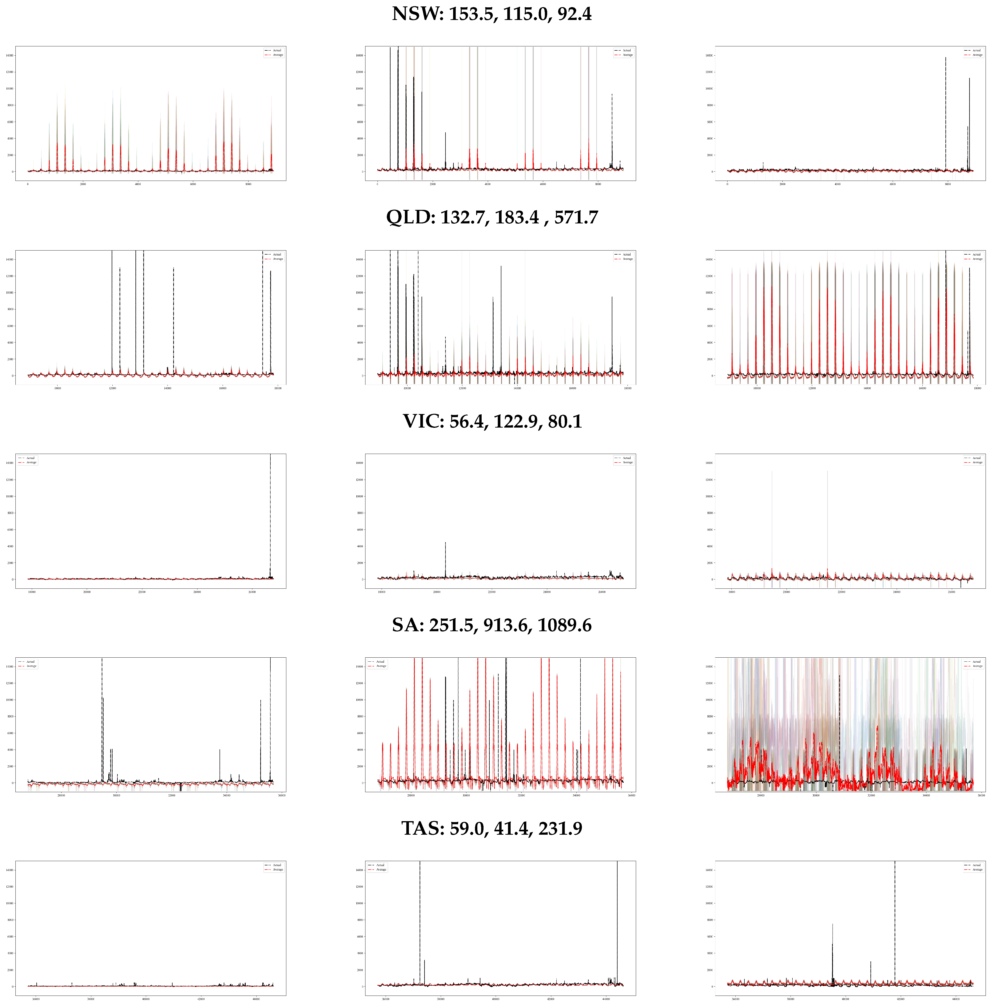
Figure 2.
Distributional results: A mid-range view. The figure shows the mid-range distributional differences between AUD −1000 and AUD 1000 of the average of the simulated 5 min prices (red) and the sample prices (black) for the three sample periods January, May, and October (left to right).
Figure 2.
Distributional results: A mid-range view. The figure shows the mid-range distributional differences between AUD −1000 and AUD 1000 of the average of the simulated 5 min prices (red) and the sample prices (black) for the three sample periods January, May, and October (left to right).
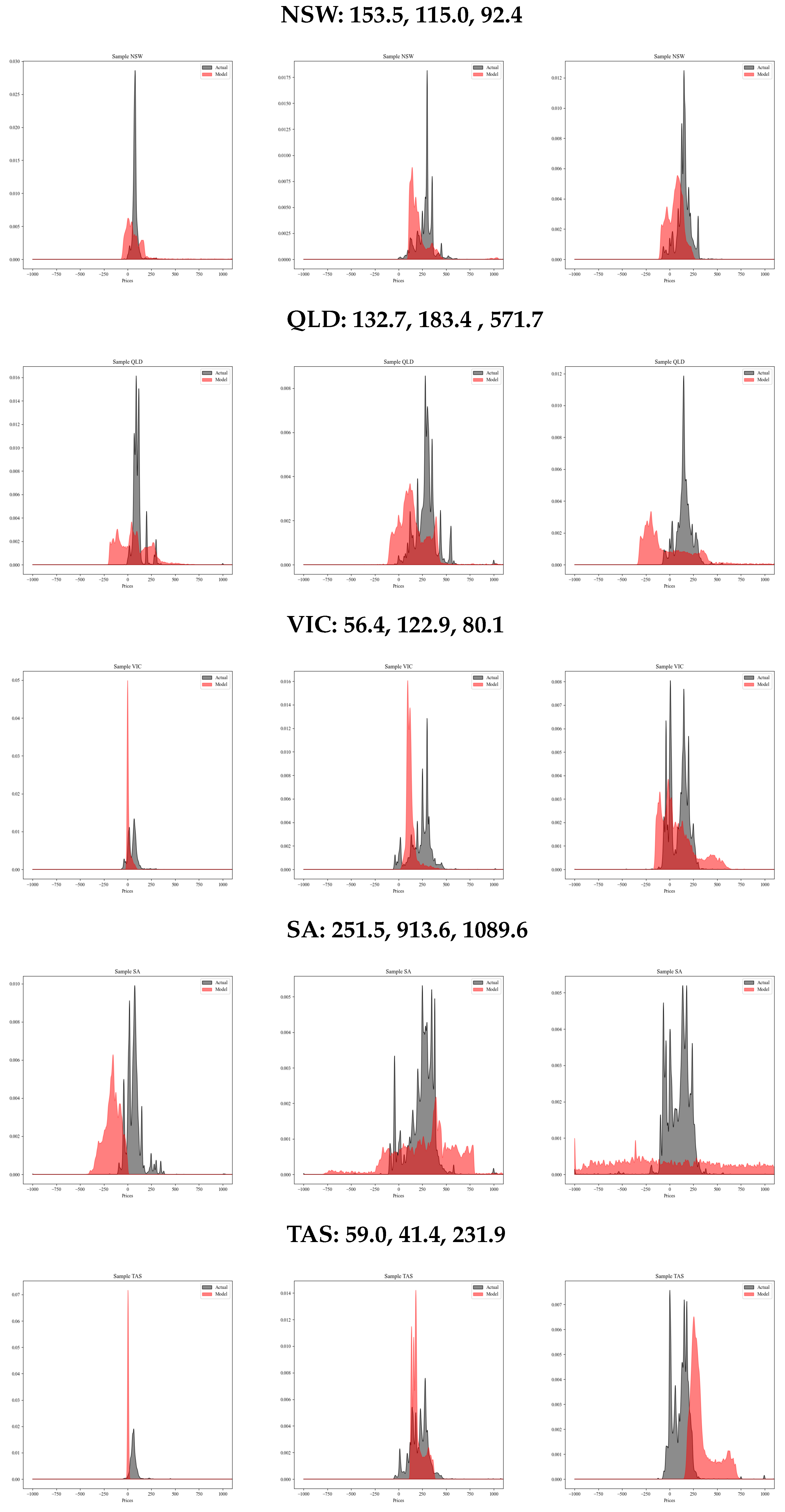
Table 1.
The fuels in the example.
| Fuel Type | Parameters | ||||||
|---|---|---|---|---|---|---|---|
| Generator fuels | |||||||
| G1 | Coal | Scheduled | 0.001 | 12.4 | 0.192 | ||
| G2 | Hydro | Scheduled | 0.001 | 47.4 | 0.002 | ||
| G3 | Solar | Scheduled | 0.001 | 150.3 | 0.043 | ||
| G4 | Gas | Scheduled | 0.001 | 131.9 | −0.041 | ||
| G5 | Biomass | Price taker | - | - | - | ||
| Load fuels | |||||||
| L1 | Battery | Scheduled | −0.001 | 48.9 | 0.000 | ||
| L2 | Hydro | Scheduled | −0.001 | 77.1 | 0.089 | ||
| Fuel type | Quantity range | Price range | |||||
| Generator fuels | |||||||
| G1 | Coal | Scheduled | 30 MW | 120 MW | AUD 0 | AUD 10 | |
| G2 | Hydro | Scheduled | 0 MW | 25 MW | AUD 0 | AUD 14 | |
| G3 | Solar | Scheduled | 0 MW | 7 MW | AUD −3 | AUD 0 | |
| G4 | Gas | Scheduled | 0 MW | 3 MW | AUD 2 | AUD 15 | |
| G5 | Biomass | Price taker | 1.5 MW | - | - | ||
| Load fuels | |||||||
| L1 | Battery | Scheduled | 0 MW | 20 MW | −$4 | $0 | |
| L2 | Hydro | Scheduled | 0 MW | 25 MW | −$2 | $0 | |
The table shows the fuels of both the regional scheduled U fuel set and the regional price taker F fuel set by type, economic classification, parameters, and quantity (in MW), and bid price (in AUD) range. The region in this example has a maximum registered generation capacity of . The parameters and are rounded to two decimal places and the to integers for every fuel . The market in the example has a market price floor of and a price cap of , but bids may appear outside that range, e.g., in fuel G4 we see the upper price at AUD 15.
Table 3.
Subset result.
| MW | MW | |||||
|---|---|---|---|---|---|---|
| Fuel Type | Subset | Dispatch Quantity | Subset | Dispatch Quantity | ||
| Generator fuels | ||||||
| G1 | Coal | Scheduled | MW | |||
| G2 | Hydro | Scheduled | MW | |||
| G3 | Solar | Scheduled | MW | MW | ||
| G4 | Gas | Scheduled | MW | 0 MW | ||
| G5 | Biomass | Price taker | - | 1.5 MW | - | 1.5 MW |
| Load fuels | ||||||
| L1 | Battery | Scheduled | - | 0 MW | ||
| L2 | Hydro | Scheduled | - | |||
| Total: MW | Total: 115 MW | |||||
The table shows the appropriate subset configuration in demand deficit scenario with end-user demand at MW (first column) and in a normal market with MW (second column). At MW, all generator and load fuels are in and , respectively, and their dispatch quantities are all shown to be constants. The total dispatch quantity also overshoots to 31.5 MW. At MW, the table shows which fuels are marginal (coal G1, hydro G2, and hydro L2) and which fuels are contributing to the constant term for the demand adjustment (solar G3), and the total dispatch quantity is exactly 115 MW. The price taker fuel (biomass G5) enjoys complete dispatch in both cases.
Table 4.
Input data.
| Model Parameter/Variable | Source (File) | Source (Field) | Data as of | Type |
|---|---|---|---|---|
| in (1) and (2) | AEMO (2023b) | PRICEBAND1-10, BANDAVAIL1-10 | See Table 5, Table 6 and Table 7 | Fitted |
| in (1) and (2) from (14)–(16) | AEMO (2023b) | PRICEBAND1-10, BANDAVAIL1-10 | 5 working days before | Fitted |
| , in (17) and (18) | AEMO (2023b) | ROCUP, ROCDOWN | ( in May) | Read off |
| m in (17) and (18) | - | - | - | Arbitrary |
| in (18) | AEMO (2023b) | MAXAVAIL, reg. cap.* | ( in May) | Read off |
| from (19) | AEMO (2023a) | EnergyTarget | 5 working days before | Randomly generated |
| from (20) | AEMO (2023a) | EnergyTarget | 5 working days before | Randomly generated |
| from (21) | AEMO (2023b) | FIXEDLOAD | ( in May) | Read off |
| from (23) | AEMO (2023a) | Price, Bids, EnergyTarget | 5 working days before | Computed, fitted |
| from (22) | NEOPoint (2023) | Dispatchable Gen | 31 days a year earlier | Fitted |
* This is calculated as the minimum of the maximum availability (MAXAVAIL in AEMO 2023b) and the registered capacity (as in AEMO 2022b) of all scheduled DUIDs in the fuel. The table shows the source of the input data together with the parametric interpretation of each field in the price algorithm.
Table 5.
Regional fuel sets—January 2022.
| Fuel | Full Bid Capacity | Ramp Speed, Multiplier | Fixed Bids | Fitting Date, Range | ||||
|---|---|---|---|---|---|---|---|---|
| NSW | ||||||||
| G1 | Black coal | Slow-start | 6340 MW | 0.05 | 0.05 | 4 | - | , [$0, $500] |
| G2 | Gravity hydro | Quick-start | 2553 MW | 0.80 | 0.80 | 4 | 65 MW | , full range |
| G3 | Natural gas | Quick-start | 1085 MW | 0.62 | 0.62 | 4 | - | , full range |
| G4 | Pumped hydro | Two-way | 160 MW | - | - | - | - | , full range |
| G5 | Battery | Two-way | 49 MW | - | - | - | - | , full range |
| L1 | Battery | Two-way | 46 MW | - | - | - | - | , full range |
| G6 | Solar | Intermittent | 2382 MW | - | - | - | - | , full range |
| G7 | Wind | Intermittent | 2237 MW | - | - | - | - | , full range |
| QLD | ||||||||
| G1 | Black coal | Slow-start | 6472 MW | 0.07 | 0.07 | 4 | - | , [$0, $500] |
| G2 | Coal seam gas | Quick-start | 1034 MW | 0.30 | 0.30 | 4 | - | , [$0, $500] |
| G3 | Kerosene | Quick-start | 395 MW | 0.41 | 0.41 | 4 | - | , full range |
| G4 | Natural gas | Quick-start | 697 MW | 0.53 | 0.53 | 4 | - | , full range |
| G5 | Run of hydro | Quick-start | 154 MW | 0.91 | 0.91 | 4 | - | , [$0, $500] |
| G6 | Pumped hydro | Two-way | 570 MW | - | - | - | - | , full range |
| G7 | Solar | Intermittent | 1692 MW | - | - | - | - | , full range |
| G8 | Wind | Intermittent | 509 MW | - | - | - | - | , full range |
| VIC | ||||||||
| G1 | Brown coal | Slow-start | 3825 MW | 0.07 | 0.07 | 4 | - | , [$0, $500] |
| G2 | Gravity hydro | Quick-start | 2165 MW | 0.62 | 0.62 | 4 | - | , [$0, $500] |
| G3 | Natural gas | Quick-start | 1758 MW | 0.48 | 0.48 | 4 | - | , full range |
| G4 | Battery | Two-way | 33 MW | - | - | - | - | , full range |
| L1 | Battery | Two-way | 80 MW | - | - | - | - | , full range |
| G5 | Solar | Intermittent | 973 MW | - | - | - | - | , full range |
| G6 | Wind | Intermittent | 3271 MW | - | - | - | - | , full range |
| SA | ||||||||
| G1 | Diesel oil | Quick-start | 253 MW | 1.44 | 1.44 | 1 | - | , [$0, $500] |
| G2 | Natural gas | Quick-start | 1029 MW | 1.05 | 1.05 | 1 | - | , [$0, $500] |
| G3 | Oil products | Quick-start | 553 MW | 0.32 | 0.32 | 1 | - | , [$0, $500] |
| G4 | Battery | Two-way | 135 MW | - | - | - | - | , full range |
| L1 | Battery | Two-way | 112 MW | - | - | - | - | , full range |
| G5 | Solar | Intermittent | 365 MW | - | - | - | - | , full range |
| G6 | Wind | Intermittent | 1923 MW | - | - | - | - | , full range |
| TAS | ||||||||
| G1 | Gravity hydro | Quick-start | 2008 MW | 1.13 | 1.13 | 1 | - | , [$0, $500] |
| G2 | Natural gas | Quick-start | 30 MW | 5.50 | 5.50 | 1 | - | , full range |
| G3 | Wind | Intermittent | 422 MW | - | - | - | - | , full range |
The table shows the scheduled fuel set of each of the five NEM regions, New South Wales (NSW), Queensland (QLD), Victoria (VIC), South Australia (SA), and Tasmania (TAS) for the third sample.
Table 6.
Regional fuel sets—May 2022.
| Fuel | Full Bid Capacity | Ramp Speed, Multiplier | Fixed Bids | Fitting Date, Range | ||||
|---|---|---|---|---|---|---|---|---|
| NSW | ||||||||
| G1 | Black coal | Slow-start | 5360 MW | 0.05 | 0.05 | 4 | - | , [$0, $500] |
| G2 | Gravity hydro | Quick-start | 2454 MW | 0.82 | 0.82 | 4 | 49 MW | , [$0, $500] |
| G3 | Natural gas | Quick-start | 1099 MW | 0.61 | 0.61 | 4 | - | , full range |
| L1 | Pumped hydro | Two-way | 160 MW | - | - | - | - | , full range |
| G4 | Battery | Two-way | 49 MW | - | - | - | - | , full range |
| L2 | Battery | Two-way | 46 MW | - | - | - | - | , full range |
| G5 | Solar | Intermittent | 2502 MW | - | - | - | - | , full range |
| G6 | Wind | Intermittent | 2225 MW | - | - | - | - | , full range |
| QLD | ||||||||
| G1 | Black coal | Slow-start | 5823 MW | 0.07 | 0.07 | 4 | - | , [$0, $500] |
| G2 | Coal seam gas | Quick-start | 870 MW | 0.36 | 0.36 | 4 | - | , [$0, $500] |
| G3 | Kerosene | Quick-start | 396 MW | 0.40 | 0.40 | 4 | - | , full range |
| G4 | Natural gas | Quick-start | 719 MW | 0.51 | 0.51 | 4 | - | , full range |
| G5 | Run of hydro | Quick-start | 132 MW | 1.06 | 1.06 | 4 | - | , full range |
| G6 | Pumped hydro | Two-way | 285 MW | - | - | - | - | , full range |
| L1 | Pumped hydro | Two-way | 244 MW | - | - | - | - | , full range |
| G7 | Solar | Intermittent | 1739 MW | - | - | - | - | , full range |
| G8 | Wind | Intermittent | 549 MW | - | - | - | - | , full range |
| VIC | ||||||||
| G1 | Brown coal | Slow-start | 3058 MW | 0.08 | 0.08 | 4 | - | , [$0, $500] |
| G2 | Gravity hydro | Quick-start | 1584 MW | 0.85 | 0.85 | 4 | - | , [$0, $500] |
| G3 | Natural gas | Quick-start | 1813 MW | 0.47 | 0.47 | 4 | - | , full range |
| G4 | Battery | Two-way | 240 MW | - | - | - | - | , full range |
| L1 | Battery | Two-way | 268 MW | - | - | - | - | , full range |
| G5 | Solar | Intermittent | 1001 MW | - | - | - | - | , full range |
| G6 | Wind | Intermittent | 2874 MW | - | - | - | - | , full range |
| SA | ||||||||
| G1 | Diesel oil | Quick-start | 269 MW | 1.36 | 1.36 | 1 | - | , full range |
| G2 | Natural gas | Quick-start | 773 MW | 0.97 | 0.97 | 1 | - | , full range |
| G3 | Oil products | Quick-start | 537 MW | 0.33 | 0.33 | 1 | - | , full range |
| G4 | Battery | Two-way | 98 MW | - | - | - | - | , full range |
| L1 | Battery | Two-way | 112 MW | - | - | - | - | , full range |
| G5 | Solar | Intermittent | 381 MW | - | - | - | - | , full range |
| G6 | Wind | Intermittent | 2152 MW | - | - | - | - | , full range |
| TAS | ||||||||
| G1 | Gravity hydro | Quick-start | 2044 MW | 1.02 | 1.02 | 1 | - | , [$0, $500] |
| G2 | Natural gas | Quick-start | 92 MW | 1.79 | 1.79 | 1 | - | , [$0, $500] |
| L1 | Battery | Two-way | 16 MW | - | - | - | - | , full range |
| G3 | Wind | Intermittent | 422 MW | - | - | - | - | , full range |
The table shows the scheduled fuel set of each of the five NEM regions, New South Wales (NSW), Queensland (QLD), Victoria (VIC), South Australia (SA), and Tasmania (TAS) for the third sample.
Table 7.
Regional fuel sets—October 2022.
| Fuel | Full Bid Capacity | Ramp Speed, Multiplier | Fixed Bids | Fitting Date, Range | ||||
|---|---|---|---|---|---|---|---|---|
| NSW | ||||||||
| G1 | Black coal | Slow-start | 6365 MW | 0.04 | 0.04 | 4 | - | , [$0, $500] |
| G2 | Gravity hydro | Quick-start | 2449 MW | 0.82 | 0.82 | 4 | 58 MW | , [$0, $500] |
| G3 | Natural gas | Quick-start | 712 MW | 0.94 | 0.94 | 4 | - | , full range |
| G4 | Pumped hydro | Two-way | 240 MW | - | - | - | - | , full range |
| L1 | Pumped hydro | Two-way | 20 MW | - | - | - | - | , full range |
| G5 | Battery | Two-way | 50 MW | - | - | - | - | , full range |
| L2 | Battery | Two-way | 51 MW | - | - | - | - | , full range |
| G6 | Solar | Intermittent | 2617 MW | - | - | - | - | , full range |
| G7 | Wind | Intermittent | 2221 MW | - | - | - | - | , full range |
| QLD | ||||||||
| G1 | Black coal | Slow-start | 5858 MW | 0.07 | 0.07 | 4 | - | , [$0, $500] |
| G2 | Coal seam gas | Quick-start | 712 MW | 0.44 | 0.44 | 4 | - | , full range |
| G3 | Kerosene | Quick-start | 276 MW | 0.58 | 0.58 | 4 | - | , full range |
| G4 | Natural gas | Quick-start | 702 MW | 0.52 | 0.52 | 4 | - | , full range |
| G5 | Run of hydro | Quick-start | 132 MW | 1.06 | 1.06 | 4 | - | , full range |
| G6 | Pumped hydro | Two-way | 524 MW | - | - | - | - | , full range |
| G7 | Battery | Two-way | 20 MW | - | - | - | - | , full range |
| L1 | Battery | Two-way | 75 MW | - | - | - | - | , full range |
| G8 | Solar | Intermittent | 2294 MW | - | - | - | - | , full range |
| G9 | Wind | Intermittent | 661 MW | - | - | - | - | , full range |
| VIC | ||||||||
| G1 | Brown coal | Slow-start | 3615 MW | 0.07 | 0.07 | 4 | - | , [$0, $500] |
| G2 | Gravity hydro | Quick-start | 1792 MW | 0.75 | 0.75 | 4 | - | , [$0, $500] |
| G3 | Natural gas | Quick-start | 1204 MW | 0.70 | 0.70 | 4 | - | , full range |
| G4 | Battery | Two-way | 295 MW | - | - | - | - | , full range |
| L1 | Battery | Two-way | 285 MW | - | - | - | - | , full range |
| G5 | Solar | Intermittent | 1015 MW | - | - | - | - | , full range |
| G6 | Wind | Intermittent | 3124 MW | - | - | - | - | , full range |
| SA | ||||||||
| G1 | Diesel oil | Quick-start | 204 MW | 1.18 | 1.18 | 1 | - | , full range |
| G2 | Natural gas | Quick-start | 822 MW | 0.91 | 0.91 | 1 | - | , full range |
| G3 | Oil products | Quick-start | 40 MW | 3.75 | 3.75 | 1 | - | , full range |
| G4 | Battery | Two-way | 117 MW | - | - | - | - | , full range |
| L1 | Battery | Two-way | 130 MW | - | - | - | - | , full range |
| G5 | Solar | Intermittent | 386 MW | - | - | - | - | , full range |
| G6 | Wind | Intermittent | 2294 MW | - | - | - | - | , full range |
| TAS | ||||||||
| G1 | Gravity hydro | Quick-start | 2044 MW | 1.08 | 1.08 | 1 | - | , [$0, $500] |
| G2 | Natural gas | Quick-start | 148 MW | 1.11 | 1.11 | 1 | - | , full range |
| G3 | Wind | Intermittent | 422 MW | - | - | - | - | , full range |
The table shows the scheduled fuel set of each of the five NEM regions, New South Wales (NSW), Queensland (QLD), Victoria (VIC), South Australia (SA), and Tasmania (TAS) for the third sample.
Table 8.
Fuel bid curve parameters—January, May, and October 2022.
| January | May | October | |||||||
|---|---|---|---|---|---|---|---|---|---|
| NSW | |||||||||
| NSWBlack coalGENERATOR | 1.99999 | 0.1 | 0.08379 | 0.35548 | 0.92 | 0.07641 | 1.09017 | 0.22 | 0.08624 |
| NSWNatural gasGENERATOR | 1.99999 | 159.79 | 0.0068 | 0.35548 | 1.44 | −0.00553 | 1.09017 | 244.67 | 0.00125 |
| NSWPumped hydroGENERATOR | 1.99999 | 333.12 | −0.00127 | 0.35548 | 19.86 | −0.08223 | 1.09017 | 981.21 | −0.00003 |
| NSWPumped hydroLOAD | — | — | — | 0.35548 | 2367.99 | 0.00371 | −1.09017 | 0.02 | 1 |
| NSWSolarGENERATOR | 1.99999 | 1851.45 | 0.05241 | 0.35548 | 1497.17 | 0.05159 | 1.09017 | 2285.51 | 0.05873 |
| NSWWindGENERATOR | 1.99999 | 185.48 | 0.04655 | 0.35548 | 434.47 | 0.04547 | 1.09017 | 1090.43 | 0.04805 |
| NSWGravity hydroGENERATOR | 1.99999 | 18.66 | 0.00239 | 0.35548 | 1.55 | −0.01212 | 1.09017 | 0.33 | −0.04448 |
| NSWBatteryGENERATOR | 1.99999 | 476.4 | −0.00003 | 0.35548 | 2136.83 | −0.00004 | 1.09017 | 570.82 | −0.00026 |
| NSWBatteryLOAD | −1.99999 | 0 | 1 | 0.35548 | 0.16 | 0.98906 | −1.09017 | 1915.19 | 0.24422 |
| QLD | |||||||||
| QLDBlack coalGENERATOR | 0.614 | 0.9 | 0.10642 | 0.54915 | 1.48 | 0.09741 | 1.73724 | 0.48 | 0.09323 |
| QLDCoal seam gasGENERATOR | 0.614 | 8.42 | 0.00036 | 0.54915 | 5.73 | −0.00122 | 1.73724 | 1679.01 | 0.00745 |
| QLDNatural gasGENERATOR | 0.614 | 285.07 | 0.01253 | 0.54915 | 787.26 | 0.01101 | 1.73724 | 201.29 | 0.00711 |
| QLDRun of hydroGENERATOR | 0.614 | 17.09 | −0.00003 | 0.54915 | 983.36 | 0.00163 | 1.73724 | 4358.63 | 0.00215 |
| QLDSolarGENERATOR | 0.614 | 1875.17 | 0.03681 | 0.54915 | 3827.84 | 0.03899 | 1.73724 | 405.74 | 0.04834 |
| QLDKeroseneGENERATOR | 0.614 | 12.41 | −0.0884 | 0.54915 | 130.63 | −0.00104 | 1.73724 | 9.07 | −0.05116 |
| QLDPumped hydroGENERATOR | 0.614 | 189.77 | 0.00631 | 0.54915 | 321.04 | 0.00343 | 1.73724 | 151.03 | −0.0003 |
| QLDPumped hydroLOAD | — | — | — | 0.54915 | 1915.19 | 0.24422 | — | — | — |
| QLDWindGENERATOR | 0.614 | 181.07 | 0.00463 | 0.54915 | 194.75 | 0.00520 | 1.73724 | 1736.17 | 0.0138 |
| QLDBatteryGENERATOR | — | — | — | — | — | — | 1.73724 | 2300.41 | −0.0002 |
| QLDBatteryLOAD | — | — | — | — | — | — | −1.73724 | 1915.19 | 0.24422 |
| VIC | |||||||||
| VICBatteryGENERATOR | 0.37907 | 2032.06 | −0.00004 | 1.30902 | 341.47 | 0.00357 | 0.38197 | 421.3 | 0.00209 |
| VICBatteryLOAD | −0.37907 | 5.26 | 0.03187 | 1.30902 | 12.59 | 0.01019 | −0.38197 | 0.05 | 1 |
| VICBrown coalGENERATOR | 0.37907 | 0.09 | 0.07338 | 1.30902 | 0.44 | 0.05840 | 0.38197 | 1.08 | 0.06282 |
| VICNatural gasGENERATOR | 0.37907 | 682.82 | 0.01303 | 1.30902 | 0.30 | −0.00715 | 0.38197 | 8.67 | −0.19373 |
| VICSolarGENERATOR | 0.37907 | 1775.27 | 0.01987 | 1.30902 | 482.08 | 0.02075 | 0.38197 | 752.42 | 0.02082 |
| VICWindGENERATOR | 0.37907 | 1039.12 | 0.06728 | 1.30902 | 441.68 | 0.05243 | 0.38197 | 364.33 | 0.06292 |
| VICGravity hydroGENERATOR | 0.37907 | 1.33 | 0.00041 | 1.30902 | 2.73 | 0.00090 | 0.38197 | 4.22 | −0.00066 |
| SA | |||||||||
| SABatteryGENERATOR | 0.32016 | 550.24 | −0.00023 | 0.21425 | 779.41 | 0.00019 | 3.29586 | 95.13 | −0.00017 |
| SABatteryLOAD | −0.32016 | 0.13 | 1 | 0.21425 | 0.22 | 1.00000 | −3.29586 | 0.01 | −1 |
| SADiesel oilGENERATOR | 0.32016 | 8.29 | −0.0072 | 0.21425 | 8.05 | −0.01433 | 3.29586 | 266.18 | −0.00035 |
| SANatural gasGENERATOR | 0.32016 | 6.13 | 0.01037 | 0.21425 | 23.68 | 0.00489 | 3.29586 | 81.33 | 0.00391 |
| SAOil productsGENERATOR | 0.32016 | 17.42 | 0.00426 | 0.21425 | 306.95 | 0.00261 | 3.29586 | 88.88 | 0.00081 |
| SAWindGENERATOR | 0.32016 | 823.46 | 0.03962 | 0.21425 | 387.09 | 0.04007 | 3.29586 | 208.4 | 0.05053 |
| SASolarGENERATOR | 0.32016 | 5428.98 | 0.00787 | 0.21425 | 9997.15 | 0.00843 | 3.29586 | 1852.37 | 0.00855 |
| TAS | |||||||||
| TASNatural gasGENERATOR | 5.377 × | 6176.97 | −0.00188 | 1.32753 | 865.44 | 0.00188 | 18.66066 | 90.66 | 0.00276 |
| TASWindGENERATOR | 5.377 × 10 | 2690.81 | 0.00397 | 1.32753 | 205.33 | 0.00624 | 18.66066 | 169.04 | 0.00623 |
| TASGravity hydroGENERATOR | 5.377 × 10 | 169.49 | −0.0254 | 1.32753 | 0.58 | 0.00571 | 18.66066 | 0.09 | 0.00849 |
| TASBatteryLOAD | — | — | — | 1.32753 | 0.01 | −0.99899 | — | — | — |
The table shows the fuel bid stack function parameters () given a regional in a NEM-wide breakdown.
Table 9.
Gamma formula inputs—Jan 2022.
| Fuel | ||||||||
|---|---|---|---|---|---|---|---|---|
| NSW | ||||||||
| NSWBlack coalGENERATOR | 0.70 | 0.18 | −0.13 | −0.84 | −0.86 | 0.05 | −4.84 | 0.17 |
| NSWNatural gasGENERATOR | 0.19 | −0.19 | −0.10 | 0.29 | −1.85 | 0.15 | −1.64 | 0.49 |
| NSWPumped hydroGENERATOR | - | - | - | - | - | - | - | - |
| NSWSolarGENERATOR | - | - | - | - | - | - | - | - |
| NSWWindGENERATOR | - | - | - | - | - | - | - | - |
| NSWGravity hydroGENERATOR | 0.01 | 0.10 | 0.13 | 3.76 | 2.37 | 0.37 | −6.00 | 0.27 |
| NSWBatteryGENERATOR | - | - | - | - | - | - | - | - |
| NSWBatteryLOAD | - | - | - | - | - | - | - | - |
| QLD | ||||||||
| QLDBlack coalGENERATOR | 0.89 | 0.02 | 0.02 | −0.78 | 2.81 | 0.38 | −1.44 | 0.28 |
| QLDCoal seam gasGENERATOR | - | - | - | - | - | - | - | - |
| QLDNatural gasGENERATOR | 0.36 | −0.34 | −0.29 | −1.00 | −3.86 | 0.17 | −0.98 | 0.68 |
| QLDRun of hydroGENERATOR | 0.01 | 0.44 | 0.30 | 2.55 | 1.48 | 2.47 | −6.00 | 0.27 |
| QLDSolarGENERATOR | - | - | - | - | - | - | - | - |
| QLDKeroseneGENERATOR | - | - | - | - | - | - | - | - |
| QLDPumped hydroGENERATOR | - | - | - | - | - | - | - | - |
| QLDWindGENERATOR | 0.35 | −0.43 | 0.43 | −3.40 | −3.41 | 3.00 | −3.10 | 0.16 |
| VIC | ||||||||
| VICBatteryGENERATOR | - | - | - | - | - | - | - | - |
| VICBatteryLOAD | 0.01 | 0.39 | 0.42 | 0.71 | −0.29 | 3.00 | −3.49 | 0.35 |
| VICBrown coalGENERATOR | 0.76 | 1.04 | −1.11 | −2.20 | −2.06 | 0.14 | −0.13 | 0.38 |
| VICNatural gasGENERATOR | 0.00 | −1.27 | 1.33 | 2.95 | 2.95 | 1.24 | −1.16 | 0.24 |
| VICSolarGENERATOR | 1.00 | −0.10 | −0.04 | 0.88 | −1.77 | 0.24 | −4.24 | 0.51 |
| VICWindGENERATOR | - | - | - | - | - | - | - | - |
| VICGravity hydroGENERATOR | 0.04 | 0.07 | −0.05 | 3.25 | 0.91 | 1.14 | −0.02 | 0.24 |
| SA | ||||||||
| SABatteryGENERATOR | 0.00 | 0.01 | −0.01 | 0.09 | −1.06 | 0.46 | −4.73 | 0.01 |
| SABatteryLOAD | 0.02 | 0.52 | −0.39 | −0.56 | −0.32 | 1.19 | −6.00 | 0.16 |
| SADiesel oilGENERATOR | 0.00 | 0.06 | −0.05 | 0.90 | 0.97 | 2.47 | −3.99 | 0.32 |
| SANatural gasGENERATOR | 0.22 | 0.08 | −0.20 | 2.77 | −1.31 | 0.28 | −0.24 | 0.21 |
| SAOil productsGENERATOR | 0.00 | 0.35 | 0.23 | 1.01 | 3.00 | 1.20 | −0.92 | 0.26 |
| SAWindGENERATOR | −0.20 | 1.20 | −0.03 | 3.82 | 2.19 | 0.00 | −5.81 | 0.13 |
| SASolarGENERATOR | - | - | - | - | - | - | - | - |
| TAS | ||||||||
| TASNatural gasGENERATOR | - | - | - | - | - | - | - | - |
| TASWindGENERATOR | 0.66 | 0.00 | −0.01 | 0.90 | 1.19 | 1.92 | −5.23 | 0.01 |
| TASGravity hydroGENERATOR | 0.58 | −0.20 | −0.09 | 0.91 | −1.12 | 1.49 | −0.43 | 0.20 |
Table 10.
Gamma formula inputs—May 2022.
| Fuel | ||||||||
|---|---|---|---|---|---|---|---|---|
| NSW | ||||||||
| NSWBlack coalGENERATOR | 0.7 | −0.06 | 0.09 | −1.38 | −3.93 | 0.9 | −1.26 | 0.23 |
| NSWNatural gasGENERATOR | 0.04 | 0.21 | 0.42 | −4 | 2.49 | 1.46 | −1.3 | 0.19 |
| NSWPumped hydroGENERATOR | - | - | - | - | - | - | - | - |
| NSWPumped hydroLOAD | - | - | - | - | - | - | - | - |
| NSWSolarGENERATOR | −0.86 | 0 | 1.83 | −2.6 | 2.42 | 0.95 | 0 | 0.08 |
| NSWWindGENERATOR | 0.99 | −0.09 | −0.02 | 4 | −2.61 | 0 | −3.53 | 0.13 |
| NSWGravity hydroGENERATOR | −0.24 | −1.93 | 2.21 | −2.16 | −2.65 | 0.04 | −0.02 | 0.12 |
| NSWBatteryGENERATOR | - | - | - | - | - | - | - | - |
| NSWBatteryLOAD | 0.02 | 0.23 | 0.2 | −0.34 | −4 | 2.37 | −0.63 | 0.12 |
| QLD | ||||||||
| QLDBlack coalGENERATOR | 0.76 | 0.13 | −0.16 | −2.67 | −2.32 | 0.11 | −0.74 | 0.32 |
| QLDCoal seam gasGENERATOR | - | - | - | - | - | - | - | - |
| QLDNatural gasGENERATOR | 0.51 | −0.31 | -0.25 | −1.98 | 0.72 | 0.32 | −5.1 | 0.21 |
| QLDRun of hydroGENERATOR | −0.95 | 0.03 | 1.51 | −1.49 | 2.35 | 1.24 | 0 | 0.02 |
| QLDSolarGENERATOR | 0.92 | −0.03 | −0.02 | 2.76 | −2.51 | 0.07 | −1.31 | 0.12 |
| QLDKeroseneGENERATOR | −0.29 | −1.75 | 2.08 | −2.23 | −2.81 | 0.04 | −0.02 | 0.13 |
| QLDPumped hydroGENERATOR | - | - | - | - | - | - | - | - |
| QLDWindGENERATOR | 0.32 | 0.15 | -0.11 | −4 | −2.81 | 0.34 | −2.22 | 0.16 |
| QLDBatteryGENERATOR | - | - | - | - | - | - | - | - |
| QLDBatteryLOAD | - | - | - | - | - | - | - | - |
| VIC | ||||||||
| VICBatteryGENERATOR | 0 | 0.23 | −0.14 | -4 | −2.87 | 0.42 | −2.36 | 0.16 |
| VICBatteryLOAD | - | - | - | - | - | - | - | - |
| VICBrown coalGENERATOR | −0.14 | 0.86 | 0.08 | 0.16 | −3.93 | 0 | −2.19 | 0.14 |
| VICNatural gasGENERATOR | 0.3 | 0.27 | 0 | 2.33 | 0.31 | 0.52 | 0.19 | 0.12 |
| VICSolarGENERATOR | −0.84 | 0.01 | 1.75 | −4 | 0.79 | 1.6 | 0 | 0.17 |
| VICWindGENERATOR | −0.98 | −0.01 | 1.85 | 1.73 | 1.22 | 2.07 | 0 | 0.12 |
| VICGravity hydroGENERATOR | 1 | −1.03 | 0.29 | 1.26 | 2.62 | 0.01 | −1.74 | 0.13 |
| SA | ||||||||
| SABatteryGENERATOR | 0.5 | −1.51 | 1.03 | 1.57 | 1.6 | 0.04 | −0.06 | 0.14 |
| SABatteryLOAD | 1 | −0.99 | −0.11 | 1.66 | −2.31 | 0.01 | −1.56 | 0.11 |
| SADiesel oilGENERATOR | 1 | −1.01 | −0.12 | 2.39 | −2.31 | 0.01 | −0.81 | 0.15 |
| SANatural gasGENERATOR | - | - | - | - | - | - | - | - |
| SAOil productsGENERATOR | 1.00 | −0.88 | −0.18 | 1.50 | −2.90 | 0.00 | −4.14 | 0.05 |
| SAWindGENERATOR | 0.88 | 0.12 | −0.12 | −1.89 | −2.10 | 0.11 | −0.23 | 0.11 |
| SASolarGENERATOR | −0.96 | 1.94 | −0.10 | −2.13 | 0.13 | 0.00 | −6.00 | 0.16 |
| TAS | ||||||||
| TASNatural gasGENERATOR | - | - | - | - | - | - | - | - |
| TASWindGENERATOR | 0.65 | −0.01 | 0.08 | -2.06 | −4.00 | 0.22 | −0.94 | 0.14 |
| TASGravity hydroGENERATOR | 0.17 | 0.15 | −0.16 | −4.00 | −2.85 | 0.45 | −2.63 | 0.10 |
| TASBatteryLOAD | - | - | - | - | - | - | - | - |
Table 11.
Gamma formula inputs—October 2022.
| Fuel | ||||||||
|---|---|---|---|---|---|---|---|---|
| NSW | ||||||||
| NSWBlack coalGENERATOR | −0.65 | 1.28 | 0.10 | 0.21 | 2.26 | 0.00 | −0.71 | 0.31 |
| NSWNatural gasGENERATOR | 0.54 | −0.55 | 0.05 | −0.73 | 2.60 | 0.01 | −4.61 | 0.36 |
| NSWPumped hydroGENERATOR | - | - | - | - | - | - | - | - |
| NSWPumped hydroLOAD | - | - | - | - | - | - | - | - |
| NSWSolarGENERATOR | - | - | - | - | - | - | - | - |
| NSWWindGENERATOR | - | - | - | - | - | - | - | - |
| NSWGravity hydroGENERATOR | 0.07 | 0.04 | 0.06 | −3.92 | 0.06 | 1.04 | −0.27 | 0.37 |
| NSWBatteryGENERATOR | 0.00 | −0.17 | 0.31 | 2.62 | 2.62 | 3.00 | −6.00 | 0.24 |
| NSWBatteryLOAD | 0.00 | 0.02 | 0.09 | −0.83 | −0.09 | 1.88 | −6.00 | 0.09 |
| QLD | ||||||||
| QLDBlack coalGENERATOR | 0.73 | −0.04 | −0.05 | 0.49 | −1.00 | 1.64 | −1.86 | 0.36 |
| QLDCoal seam gasGENERATOR | 0.00 | 0.14 | 0.27 | 4.00 | 2.84 | 0.44 | −1.94 | 0.61 |
| QLDNatural gasGENERATOR | 0.40 | −0.37 | −0.30 | −2.83 | 0.56 | 0.15 | −1.33 | 0.42 |
| QLDRun of hydroGENERATOR | 0.68 | −0.79 | −0.75 | −4.00 | −0.15 | 0.71 | −0.52 | 0.74 |
| QLDSolarGENERATOR | - | - | - | - | - | - | - | - |
| QLDKeroseneGENERATOR | - | - | - | - | - | - | - | - |
| QLDPumped hydroGENERATOR | - | - | - | - | - | - | - | - |
| QLDWindGENERATOR | 0.93 | −1.27 | 1.08 | −0.42 | −0.44 | 1.05 | −0.97 | 0.47 |
| VIC | ||||||||
| VICBatteryGENERATOR | 0.00 | 0.00 | 0.00 | 0.41 | 1.74 | 2.47 | −5.20 | 0.04 |
| VICBatteryLOAD | 0.00 | 0.17 | 0.18 | 0.19 | −3.55 | 1.06 | −2.04 | 0.21 |
| VICBrown coalGENERATOR | 0.77 | 0.06 | 0.06 | 0.72 | −0.56 | 0.64 | −2.93 | 0.11 |
| VICNatural gasGENERATOR | 0.01 | 2.25 | −2.06 | 2.30 | 2.19 | 0.43 | −0.45 | 0.65 |
| VICSolarGENERATOR | - | - | - | - | - | - | - | - |
| VICWindGENERATOR | - | - | - | - | - | - | - | - |
| VICGravity hydroGENERATOR | −0.35 | −0.30 | 0.99 | 1.88 | 0.17 | 0.74 | −0.02 | 0.20 |
| SA | ||||||||
| SABatteryGENERATOR | −0.72 | −1.62 | 2.34 | −3.17 | −3.81 | 0.00 | 0.00 | 0.02 |
| SABatteryLOAD | 0.01 | 0.07 | 0.09 | −3.23 | 1.04 | 2.60 | −0.89 | 0.12 |
| SADiesel oilGENERATOR | 0.00 | 0.04 | 0.03 | 1.00 | −0.62 | 3.00 | −6.00 | 0.25 |
| SANatural gasGENERATOR | 0.20 | −3.00 | 2.79 | 1.02 | 1.13 | 0.25 | −0.20 | 0.62 |
| SAOil productsGENERATOR | - | - | - | - | - | - | - | - |
| SAWindGENERATOR | - | - | - | - | - | - | - | - |
| SASolarGENERATOR | - | - | - | - | - | - | - | - |
| TAS | ||||||||
| TASNatural gasGENERATOR | 0.25 | −0.21 | 0.13 | −3.04 | −0.01 | 0.34 | −1.03 | 0.14 |
| TASWindGENERATOR | 0.65 | −0.01 | 0.01 | 1.43 | 1.62 | 2.02 | −5.26 | 0.01 |
| TASGravity hydroGENERATOR | 0.49 | 0.04 | −0.07 | −0.24 | 2.93 | 0.32 | −0.54 | 0.32 |
Table 12.
Solar availability formula inputs.
| January 2022 | |||||||
|---|---|---|---|---|---|---|---|
| Region | a | b | c | d | e | f | g |
| NSW | 0.0000 | 0.0150 | −1.0000 | −0.9920 | 0.0000 | −0.5818 | 0.8 |
| QLD | −0.0007 | 0.0152 | −0.5354 | −0.3525 | −0.1253 | −0.5746 | 0.5 |
| VIC | −3.18 × | 1.78 × | 1.16 × | −5.36 × | −4.73 × | −8.92 × | 0.2 |
| SA | −0.0020 | 0.0119 | −0.0184 | 0.1870 | −0.2785 | −0.1330 | 0.1 |
| May 2022 | |||||||
| Region | a | b | c | d | e | f | g |
| NSW | −1.35 × | 1.55 × | 1.81 × | −9.57 × | −1.95 × | −2.49 × | 0.5 |
| QLD | −0.0008 | 0.0152 | −0.2712 | −0.1369 | −0.1450 | −0.5905 | 0.35 |
| VIC | −4.10 × | 1.86 × | 4.36 × | −4.02 × | −6.09 × | −8.61 × | 0.15 |
| SA | −0.0021 | 0.0058 | 0.4605 | −0.3066 | −0.2906 | −0.1429 | 0.1 |
| October 2022 | |||||||
| Region | a | b | c | d | e | f | g |
| NSW | −5.00 × | 1.55 × | −9.99 × | −9.99 × | −4.36 × | −9.99 × | 0.75 |
| QLD | −4.67 × | 1.53 × | −3.19 × | −9.49 × | −3.55 × | −4.58 × | 0.6 |
| VIC | −3.76 × | 1.83 × | 3.15 × | −4.53 × | −5.57 × | −8.73 × | 0.2 |
| SA | −0.0020 | 0.0119 | −0.2359 | 0.0365 | −0.2785 | −0.1078 | 0.125 |
The table shows the solar generation upper bound quantity (19) inputs of the relevant NEM regions: New South Wales (NSW), Queensland (QLD), Victoria (VIC), and South Australia (SA).
Table 13.
Wind availability formula inputs.
| January 2022 | May 2022 | October 2022 | |||||||
|---|---|---|---|---|---|---|---|---|---|
| Region | |||||||||
| NSW | 18.205 | 0.6 | 0.2 | 14.964 | 0.6 | 0.2 | 20.404 | 0.6 | 0.2 |
| QLD | 11.288 | 0.6 | 0.2 | 11.466 | 0.6 | 0.2 | 13.872 | 0.6 | 0.2 |
| VIC | 42.212 | 0.6 | 0.2 | 25.255 | 0.6 | 0.2 | 30.155 | 0.6 | 0.2 |
| SA | 21.921 | 0.4 | 0.2 | 25.077 | 0.4 | 0.2 | 21.354 | 0.4 | 0.2 |
| TAS | 6.162 | 0.6 | 0.2 | 7.687 | 0.6 | 0.2 | 6.027 | 0.6 | 0.2 |
The table shows the wind generation upper bound quantity (20) inputs of the five NEM regions: New South Wales (NSW), Queensland (QLD), Victoria (VIC), South Australia (SA), and Tasmania (TAS).
Table 14.
Constrained-on/off formula inputs.
| January 2022 | May 2022 | October 2022 | ||||
|---|---|---|---|---|---|---|
| Region | ||||||
| NSW | 0.1 | 4.60 | 0.1 | 5.68 | 0.1 | 7.11 |
| QLD | 0.1 | 5.25 | 0.1 | 5.43 | 0.1 | 5.30 |
| VIC | 0.25 | 9.84 | 0.25 | 3.02 | 0.25 | 3.17 |
| SA | 0.1 | 1.20 | 0.1 | 0.65 | 0.1 | 0.79 |
| TAS | 0.25 | 4.68 | 0.25 | 3.80 | 0.25 | 7.00 |
The table shows the inputs of the constrained-on/off quantity in (24) over the three periods for the five NEM regions: New South Wales (NSW), Queensland (QLD), Victoria (VIC), South Australia (SA), and Tasmania (TAS).
Table 15.
Generation formula inputs.
| January 2022 | |||||||||||
|---|---|---|---|---|---|---|---|---|---|---|---|
| Fuel | |||||||||||
| NSW | 0.83 | −0.06 | 0.64 | 1.10 | 0.48 | −0.25 | 1.65 | 0.76 | 0.13 | −0.43 | 0.53 |
| QLD | 0.88 | −0.03 | 0.56 | 1.14 | 0.26 | 0.00 | 2.62 | 0.87 | 0.24 | 1.43 | 0.75 |
| VIC | 0.74 | −0.02 | 1.46 | 1.19 | 0.15 | −0.01 | 2.81 | 1.09 | 0.53 | −0.91 | 0.26 |
| SA | 0.14 | −0.01 | 1.02 | 1.04 | 0.06 | 0.00 | 3.02 | 0.78 | 0.56 | 1.05 | 0.22 |
| TAS | 0.09 | 0.00 | 1.01 | 1.14 | 0.05 | 0.00 | 3.01 | 0.78 | 0.68 | 1.05 | 0.22 |
| May 2022 | |||||||||||
| Fuel | |||||||||||
| NSW | 0.90 | −0.05 | −10.78 | 1.16 | 0.61 | −0.54 | 1.28 | 0.77 | 0.12 | −0.43 | 0.56 |
| QLD | 0.84 | 0.03 | −2.39 | 1.13 | 0.24 | 0.00 | 2.88 | 0.82 | 0.59 | 1.27 | 0.55 |
| VIC | 0.72 | 0.04 | −2.43 | 1.13 | 0.19 | 0.00 | 2.90 | 0.91 | 0.83 | 1.02 | 0.42 |
| SA | 0.16 | −0.01 | 1.01 | 1.28 | 0.09 | 0.00 | 3.02 | 0.78 | 0.97 | 1.05 | 0.32 |
| TAS | 0.16 | −0.02 | 1.01 | 1.27 | 0.10 | 0.00 | 2.94 | 0.78 | 0.59 | 1.05 | 0.37 |
| October 2022 | |||||||||||
| Fuel | |||||||||||
| NSW | 0.82 | −0.06 | −27.91 | 1.15 | 0.57 | −0.57 | 1.30 | 0.65 | 0.15 | −0.31 | 0.59 |
| QLD | 0.80 | 0.03 | 1.49 | 1.17 | 0.25 | 0.00 | 2.82 | 0.85 | 0.47 | 1.38 | 0.69 |
| VIC | 0.67 | 0.03 | −13.05 | 1.11 | 0.16 | −0.11 | 3.00 | 0.34 | 1.08 | −0.58 | 0.57 |
| SA | 0.14 | −0.02 | 1.01 | 1.27 | 0.02 | 0.00 | 3.18 | 0.78 | 1.01 | 1.05 | 0.09 |
| TAS | 0.16 | 0.01 | 1.01 | 1.27 | 0.08 | 0.00 | 3.18 | 0.78 | 0.88 | 1.05 | 0.24 |
The table shows the inputs of the generation quantity in (22) over the three periods for the five NEM regions: New South Wales (NSW), Queensland (QLD), Victoria (VIC), South Australia (SA), and Tasmania (TAS).
Table 16.
Wasserstein distances.
| Actual Prices | Modelled Prices | |||||
|---|---|---|---|---|---|---|
| Region | January–May | May–October | January–October | January | May | October |
| NSW | 243.6 | 169.4 | 81.6 | 153.5 | 115.0 | 92.4 |
| QLD | 211.3 | 194.0 | 79.7 | 132.7 | 183.4 | 571.7 |
| VIC | 189.7 | 135.5 | 68.9 | 56.4 | 122.9 | 80.1 |
| SA | 223.8 | 219.4 | 74.7 | 251.5 | 913.6 | 1089.6 |
| TAS | 154.1 | 104.9 | 71.6 | 59.0 | 41.4 | 231.9 |
The table shows the Wasserstein distances between the actual price series (first column) and between the modelled price averages of 25 iterations and the actual price series. Cases where the distance to model is approximately the same or less than the distances between the empirical distributions are highlighted in bold.
Disclaimer/Publisher’s Note: The statements, opinions and data contained in all publications are solely those of the individual author(s) and contributor(s) and not of MDPI and/or the editor(s). MDPI and/or the editor(s) disclaim responsibility for any injury to people or property resulting from any ideas, methods, instructions or products referred to in the content. |
© 2023 by the authors. Licensee MDPI, Basel, Switzerland. This article is an open access article distributed under the terms and conditions of the Creative Commons Attribution (CC BY) license (https://creativecommons.org/licenses/by/4.0/).
Share and Cite
MDPI and ACS Style
Katona, K.; Nikitopoulos, C.S.; Schlögl, E. A Hyperbolic Bid Stack Approach to Electricity Price Modelling. Risks 2023, 11, 147. https://doi.org/10.3390/risks11080147
AMA Style
Katona K, Nikitopoulos CS, Schlögl E. A Hyperbolic Bid Stack Approach to Electricity Price Modelling. Risks. 2023; 11(8):147. https://doi.org/10.3390/risks11080147
Chicago/Turabian StyleKatona, Krisztina, Christina Sklibosios Nikitopoulos, and Erik Schlögl. 2023. "A Hyperbolic Bid Stack Approach to Electricity Price Modelling" Risks 11, no. 8: 147. https://doi.org/10.3390/risks11080147
Note that from the first issue of 2016, this journal uses article numbers instead of page numbers. See further details here.