
A Comparison of Generalised Linear Modelling with Machine Learning Approaches for Predicting Loss Cost in Motor Insurance


1
School of Computing, Birmingham City University, Birmingham B4 7RQ, UK
2
National Farmers Union Mutual Insurance Society, Tiddington, Stratford-upon-Avon CV37 7BJ, UK
*
Author to whom correspondence should be addressed.
†
These authors contributed equally to this work.
Risks 2024, 12(4), 62; https://doi.org/10.3390/risks12040062
Submission received: 17 February 2024
/
Revised: 27 March 2024
/
Accepted: 28 March 2024
/
Published: 31 March 2024
Abstract
:This study explores the insurance pricing domain in the motor insurance industry, focusing on the creation of “technical models” which are essentially obtained after combining the frequency model (the expected number of claims per unit of exposure) and the severity model (the expected amount per claim). Technical models are designed to predict the loss costs (the product of frequency and severity, i.e., the expected claim amount per unit of exposure) and this is a main factor that is taken into account for pricing insurance policies. Other factors for pricing include the company expenses, investments, reinsurance, underwriting, and other regulatory restrictions. Different machine learning methodologies, including the Generalised Linear Model (GLM), Gradient Boosting Machine (GBM), Artificial Neural Networks (ANN), and a unique hybrid model that combines GLM and ANN, were explored for creating the technical models. This study was conducted on the French Motor Third Party Liability datasets, “freMTPL2freq” and “freMTPL2sev” included in the R package CASdatasets. After building the aforementioned models, they were evaluated and it was observed that the hybrid model which combines GLM and ANN outperformed all other models. ANN also demonstrated better predictions closely aligning with the performance of the hybrid model. The better performance of neural network models points to the need for actuarial science and the insurance industry to look beyond traditional modelling methodologies like GLM.
1. Introduction
The financial services industry, especially its most prominent and visible member—Insurance—is undergoing a rapid and disruptive change fueled by advanced technologies and changing consumer needs. The insurance sector is on the brink of a digital revolution, transforming the way it conducts business, by leveraging advanced data analytical capabilities as a primary driver Garrido et al. (2016). The amount of data generated by the industry is huge and all the companies realising the potential benefits that data analysis can bring to them are investing billions into enhancing their data analytical techniques.
The insurance industry is unique because it manages the risks and uncertainties associated with unforeseeable events. Insurance companies offer the service of covering unpredictable events, as per their terms and conditions, in exchange for an annual sum (the insurance premium) to be paid by the customer Poufinas et al. (2023). Instead of knowing the precise cost up front, the pricing of insurance products is based on calculating the prospective losses that could occur in the future Kleindorfer and Kunreuther (1999). Insurance firms have long used mathematics and statistical analysis to make these estimations. Statistical methods have been used in the different subdivisions of the insurance sector, including motor, life, and general insurance, to ensure that the premiums charged to the customers are enough to maintain the financial solvency of the company while meeting its profit targets.
Motor insurance pricing is based on the risk factors of the policyholder, such as the age of the driver, the power of the vehicle, or the address where the policyholder resides in the case of auto insurance. Using these features, an actuary generates groups of policyholders with corresponding risk assessments. In addition to the static risk factors, insurance companies take the vehicle use into account, including the frequency of use and the area, when finalising the risk premiums Vickrey (1968); Henckaerts and Antonio (2022). In this paper, the focus is on motor insurance, but the findings are applicable to other divisions due to the common practices for determining the risk Wüthrich and Merz (2022).
Uncertainty is the core of the insurance business, which makes stochastic modelling suitable for forecasting various outcomes from different random attributes Draper (1995). Creating a stochastic model to facilitate decision-making and risk assessment in the insurance industry requires the analysis of historical data for forecasting future costs for an insurance policy. Data mining can be used to retrieve this vital information. Risk clustering is an approach in data mining which can help create large, similar, and different groups within and between classes Smith et al. (2000).
Actuarial science is a discipline that analyses data, assesses risks, and calculates probable loss costs for insurance policies using a range of mathematical models and methods Dhaene et al. (2002). Actuaries consider information from the past, including demographics, medical records, and other relevant factors to create precise risk profiles for specific people or groups that have a similar potential outcome. The main challenge for actuaries lies in the modelling of the frequency of claims. When a person applies for a car insurance policy, forecasting the frequency of claims plays is a major factor in the classification of the candidate within a certain risk profile David (2015). Claims severity (the amount for each claim) is another factor that determines the exposure of the insurance company if a policy if offered Mehmet and Saykan (2015). Multiplying the number of claims (the frequency) with the average amount per claim (the severity) reflects the cost of the claims on the insurance company. Combining frequency and severity models enables the prediction of loss costs Garrido et al. (2016). These predictions, however, are referred to as “technical models” in the insurance industry, as they do not take into account other external factors including inflation, regulatory constraints, and practices followed to insure customer retention. Factors such as expenses, investments, reinsurance, and other model adjustments and regulatory constraints assist in arriving at the final premium amount Tsvetkova et al. (2021); Shawar and Siddiqui (2019). Developing the best possible “technical models” is essential for an insurance company to enable the prediction of appropriate insurance premiums Guelman (2012), and this is the focus of this paper.
Typically, insurance companies rely on statistical models that enable having a level of transparency required to justify the pricing for the regulatory body and customer when needed. Generalised Linear Model (GLM) is the leading technique that is used for pricing in the insurance industry due to its ease of interpretability and ability to give a clear understanding of how each predictor affects the outcome for pricing Zheng and Agresti (2000). GLM, however, suffers from several shortfalls, especially with the increase in the amount of data that are considered when building the models; these shortfalls include the following:
- The time inefficiency for updating the GLM models in light of new data, as common practices followed by actuaries require manual steps in the fine-tuning of the weights of each factor.
- The dependence of GLM on assumptions on the distribution of the data, which are not always valid for datasets representing an unusual market, for example, due to a certain phenomenon impacting the behaviour of customers King and Zeng (2001).
- The unsuitability of GLM for modelling non-linear complex trends Xie and Shi (2023).
These factors are among the reasons that have driven insurance companies to start exploring machine learning techniques for pricing Poufinas et al. (2023). Machine learning, however, is only meant to support and not substitute GLM modelling due to the black box nature of some machine learning algorithms and the opaqueness of the produced models, rendering the justification of the impact of every factor on the prediction to regulatory bodies difficult Rudin (2019). Actuaries are now exploring the use of machine learning techniques to find a balance between the improved accuracy that can be achieved and the transparency offered by GLM Lozano-Murcia et al. (2023). In this paper, we explore some of these techniques and compare their performance with GLM. We also used a hybrid model that factors in the prediction of the frequency and severity of claims from a GLM model as an attribute for the Artificial neural network model. The rest of this paper is structured as follows: Section 2 discusses related work and highlights the need for this study; Section 3 describes the dataset and discusses the theoretical background related to the different steps of the knowledge discovery process; Section 4 elaborates on these steps and discusses the hyperparameter tuning of the models; Section 5 includes the results and discussion of the findings, and Section 6 concludes the paper and gives directions for future work.
2. Literature Review
Generalised Linear Modelling (GLM) methods have been a standard industry practice for non-life insurance pricing for a long time now Xie and Shi (2023). The monograph created by Goldburd et al. (2016) serves as a reference for the use of GLMs in classification rate-making. They have built a classification plan from raw premium and loss data. Kafková and Křivánková (2014) analysed motor insurance data using GLM and created a model for the frequency of claims. The performance of the models was compared using the Akaike information criterion (AIC) and Analysis of Deviance. However, AIC accounts for penalising complexity, giving a disadvantage to models with a large number of relevant parameters. This model presents a relatively simple model and validates the significance of three variables in the prediction process: the policyholder’s age group, the age of the vehicle, and the location of residency.
Garrido et al. (2016) used generalised linear models to calculate the premium by multiplying the mean severity, mean frequency, and a correction term intended to induce dependency between these components on a Canadian automobile insurance dataset. This method assumes a linear relationship between average claim size and the number of claims which may not hold in all cases Xie and Shi (2023). David (2015) also discusses the usefulness of GLMs for estimating insurance premiums based on the product of the expected frequency and claim costs. The authors of these papers, however, did not explore other models that are suitable for more complex non-linear trends.
Moreover, it has been established that the Poisson models are commonly employed in GLM approaches within the insurance industry to predict claim frequency. Throughout the literature, multiple authors have stated that the Poisson model is the main method for forecasting the frequency of claims in the non-life insurance sector Denuit and Lang (2004); Antonio and Valdez (2012); Gourieroux and Jasiak (2004); Dionne and Vanasse (1989). For the claim severity model, the literature asserts that the Gamma model is the conventional approach for modelling claim costs David (2015); Pinquet (1997).
Xie and Shi (2023) stated that it is simpler to choose key features or measure the significance of the features in linear models when compared to decision-tree-based techniques or neural networks Xie and Shi (2023). However, they also asserted the fact that GLM is unable to recognise complex or non-linear interactions between risk factors and the response variable. As these would affect the pricing accuracy, they stated the necessity of considering alternate solutions, which includes the complicated non-linear models.
Zhang (2021) performed a comparative analysis to evaluate the impact of machine learning techniques and generalised linear models on the prediction of car insurance claim frequency Zhang (2021). Seven insurance datasets were used in the extensive study, which employed the standard GLM approach, XGboost, random forest, support vector machines, and deep learning techniques. According to the study, XGboost predictions outperformed GLM on all datasets. Another recent study by Panjee and Amornsawadwatana (2024) confirmed that XGboost outperformed GLMs for frequency and severity modelling in the context of cargo insurance. Guelman (2012) used the Gradient Boost Machine (GBM) method for auto insurance loss cost modelling and stated that while needing little data pre-processing and parameter adjustment, GBM produced interpretable results Guelman (2012). They performed feature selection then produced a GBM model capturing the complex interactions in the dataset, resulting in higher accuracy than that obtained from the GLM model. Poufinas et al. (2023) also suggested that tree-based models performed better than alternative learning techniques; their dataset, however, was limited to 48 instances and their results were not compared to GLM Poufinas et al. (2023).
Also, in the existing literature, multiple papers supported the use of neural network algorithms in the insurance industry. Many experiments have been done on the use of neural networks in insurance pricing and these studies concluded that these models resulted in a higher accuracy than traditional models like GLM Bahia (2013); Yu et al. (2021). In 2020, a study was conducted on French Motor Third-Party Liability claims, and methods such as regression trees, boosting machines, and feed-forward neural networks were benchmarked against a classical Poisson generalised linear model Noll et al. (2020). The results showed that methods other than GLM were able to capture the feature component interactions appropriately, mostly because GLMs require extended manual feature pre-processing. They also emphasised the importance of ‘neural network boosting’ where the advanced GLM model is nested into a bigger neural network Schelldorfer et al. (2019). Schelldorfer et al. (2019) discussed the importance of embedding classical actuarial models like GLM into a neural net, known as the Combined Actuarial Neural Net (CANN) approach Schelldorfer et al. (2019). While doing so, CANN captures complex patterns and non-linear relationships in the data, whereas the GLM layer accounts for specific actuarial assumptions. Using a skip connection that directly connects the neural network’s input layer and output layer, the GLM is integrated into the network architecture. This strategy makes use of the capabilities of neural networks to improve the GLM, and this is referred to as a hybrid model.
Hybrid models are popular nowadays as they combine the output of multiple models and produce more accurate results compared to single models Ardabili et al. (2019). The fundamental principle underlying hybrid modelling is to combine the outputs of various models in order to take advantage of their strengths and minimise their flaws, thus improving the robustness and accuracy of predictions Zhang et al. (2019); Wu et al. (2019).
From the literature review, it can be deduced that numerous publications support the traditional GLM model in the existing literature. GLM accounts for the popular and most common data mining method in the insurance industry. It has been clear that the GLM models are still effective models because of their flexibility, simple nature, and ease of implementation. However, GLM cannot handle diverse datatypes and does not work well in dealing with non-linear relationships in the data. Due to these drawbacks of the GLM model, there are multiple works in the literature that support the Gradient Boost Machines (GBM) model since it ensures model interpretability through its feature selection capabilities. The literature review also highlights the importance of the neural network approach, as it shows better and more reliable results than traditional models. The literature demonstrates that hybrid models work more effectively than single models and suggests that combining GLM and neural network performs better as it aids in maximising the advantages of both techniques. This was proven by Schelldorfer et al. (2019), whose CANN approach showed reliable results by capturing complex patterns and non-linear relationships in the data, while also including actuarial assumptions specific to the insurance industry. While reviewing the literature, it was noted that the methods such as random forests and support vector machines are not frequently used for the calculation of claim frequency and severity. This may be because these techniques require significant computational effort and training.
Building on the findings from the literature, this study aims to explore the effectiveness of Combined Actuarial Neural Networks (CANN) in comparison with GLM, GBM, and artificial neural networks models. Compared to the work of Noll et al. (2020); Schelldorfer et al. (2019), our work is the first to compare these four models together and discuss the findings to help guide the actuarial community on finding the needed tradeoff between accuracy and transparency. Our work covers twelve models with different sets of features and details every step of the Knowledge Discovery from Databases (KDD) process from the data preparation and cleaning to the analysis and comparison of the results of our models. Compared to other work in the literature, this paper focuses on motor insurance pricing models, but the findings are extendable to other insurance subdivisions.
3. Theoretical Background
This section introduces the dataset and the various steps that are followed to build the model. The steps described below are aligned with the Knowledge Discovery from Databases (KDD) process, due to the significance and importance of this methodology for building the best possible models Fayyad et al. (1996).
3.1. Dataset Source and Description
The outcomes of the project can be impacted by an appropriate dataset. An important step in this project was finding and selecting a suitable dataset that could be utilised in achieving the project’s objective. Thorough research was necessary since there was a need to find the Insurance dataset, which includes frequency and severity counterparts as well. After in-depth research, the French Motor Third-Party Liability datasets “freMTPL2freq” and “freMTPL2sev” included in the R package CASdatasets were found for claim frequency modelling and claim severity modelling Dutang and Charpentier (2020). These datasets contain the risk characteristics gathered over one year for 677,991 motor vehicle third-party liability insurance policies. While freMTPL2freq comprises the risk characteristics and the claim number, freMTPL2sev provides the claim cost and the associated policy ID Dutang and Charpentier (2020).
Table 1 and Table 2 list the attributes of the fremMTPL2freq and freMTPL2sev datasets along with each feature’s description and data type. The freMTPL2freq dataset contains 678,013 individual car insurance policies and for each policy there are 12 variables associated with it. The freMTPL2sev dataset includes 26,639 observations of claim amounts and corresponding policy IDs. Both datasets were merged, and the entire the analysis and model building was conducted on that.
3.2. Data Cleaning and Pre-Processing
Data cleaning and pre-processing is one of the crucial steps as unprocessed and incomplete data cannot produce good results. It is widely acknowledged that the success of each data mining method is significantly influenced by the standard of data pre-processing Miksovsky et al. (2002). The data may, however, include mismatched data types, outliers, imbalances, missing numbers, etc., if they have not been properly pre-processed. The pre-processing steps employed in the study are described here.
After merging the frequency and severity datasets, they are thoroughly pre-processed. The steps taken during the initial pre-processing stage are listed below:
- NA values for severity after merging the datasets are changed to zero, where the left join of the frequency and severity datasets resulted in records with 0 claims having no equivalent severity records (leading to NA values).
- Duplicate rows (exact duplicates) have been removed, as those were deemed to be data entry errors.
- The dataset was filtered to eliminate any rows with claim amounts equal to zero. This is because removing claims with zero amount improves the performance of the severity data. Also, within the severity dataset, the claim amounts up to the 97th percentile were zeroes.
- Upon observing the data, it was found that there was a substantial difference between the value at the 99.99th percentile blue (974,159) and the 100th percentile (4,075,400). Claim amounts beyond the 99.99th percentile constitute approximately 14% of the total claim amount and can be considered as an extreme value. Hence, the claim amount at the 99.99th percentile is set as a threshold value and claim amounts above the 99.99th percentile are limited to the corresponding value at the same percentile.
Two different approaches have been followed in the pre-processing for the models.
Pre-processing steps for GLM and GBM are outlined as follows:
- Convert the categorical variables ‘Area’ and ‘VehGas’ into factors and then into a numeric format.
- Convert the variables ‘VehBrand’, and ‘Region’ into factors.
- Convert the ‘Density’ variable into the numeric format and ‘BonusMalus’ into integer format.
- Variable ‘ClaimNb’ is modified into double format.
The pre-processing steps followed for ANN are as follows:
- Perform Min-Max Scaling for numerical features ‘VehPower’, ‘VehAge’, ‘DrivAge’, ‘BonusMalus’, ‘Density’.
- Execute One-Hot Encoding for categorical features ‘Area’ and ‘VehGas’, ‘VehBrand’, and ‘Region’.
- Variable ‘ClaimNb’ is modified into double format.
3.3. Exploratory Data Analysis
Exploratory data analysis (EDA) is an essential step in any research analysis as it aims to examine the data for outliers, anomalies, and distribution patterns and helps to visualise and understand the data Komorowski et al. (2016). In this research paper, most of the visualisations would be bar charts due to the importance of studying the distribution of a dataset prior to settling on a modelling technique. Detailed exploratory analysis is shown in the following subsections.
3.3.1. Analysis of Risk Features
It is necessary to examine the nature of the risk features, and if there are any irregularities with their structure, these need to be corrected. This section describes the modifications that were made to the risk features after looking at their distribution.
It was observed that there were 1227 entries in the dataset for which the exposures were greater than 1. According to Dutang and Charpentier (2020), all observations were made within one accounting year; hence, these exposures above 1 may have been the result of a data error and were corrected to 1.
The distribution of the feature variable ‘Exposure’ before and after the cap is depicted in Figure 1 and Figure 2.
Vehicle age is an important feature in the context of insurance analysis. Figure 3 shows the number of observations and the frequency of claims per vehicle age before capping. Looking at the trend of the frequency and the count, it can be observed that the trend is volatile and the data are scarce after the value of 20. Further inspection of the data shows that 98.7% of the insured vehicles are captured within a range of 20 for vehicle age.
Therefore, to ensure the integrity of this feature, a capping mechanism was put in place that set the ’Vehicle Age’ values at a maximum of 20 years. Figure 3 and Figure 4 show the distribution of ‘Vehicle Age’ before and after the cap. Figure 4 shows that the trend after capping is more consistent.
Figure 5 is a bar plot showing the number of observations and the frequency of claims for each value of driver age. The trend line is volatile after 85, but the plot shows further scarcity of the data points after 90. To ensure that we do not miss any underlying trends at both ends of the data, we decided to cap “DrivAge” at 90, covering 99.9% of the dataset. Figure 5 and Figure 6 show the distribution of ‘driver age’ before and after the cap.
Figure 7 is a bar plot showing the number of observations and the frequency of claims for different values of vehicle power in our dataset. The figure shows that our data are scarce after 13 and the trend line for the frequency becomes more volatile starting at this value. We capped Vehicle Power at 13, which covers 99.2% of the dataset. Figure 7 and Figure 8 show the distribution of the feature before and after the capping.
Figure 9 is a bar plot showing the frequency of claims and the number of observations for each value of BonusMalus. The figure shows an increase in the volatility in frequency and an increase in the scarcity of the observations after the value of 150. We capped BonusMalus at 150 covering 99.96% of the data, thus ensuring that both the Bonus (values less than 100) and Malus (values over 100) are captured when building the models. Figure 10 shows the distribution of the BonusMalus values with respect to the frequency and number of claims after capping.
The feature ‘ClaimNb’ indicates that there are a few policies that have more than 4 claims, with 16 being the most. These are rectified by setting them equal to 4, as they are likely data errors given that the data were gathered over the course of a year. Figure 11 and Figure 12 show the distributions of the feature ‘ClaimNb’ before and after capping it.
A sensitivity study will be conducted to understand the impact of the capping of the variables discussed in the section on the prediction. This will be done by training our models on the dataset with the uncapped variables and on the one with the variables after capping. This will help us assess if the changes to the input variable will help in improving the predictive capability of the models. More details about this analysis are included in Section 5.
3.3.2. Analysing the Relationship between Variables
As part of analysing the data, the association between the age of the driver and the number of insurance claims was examined and is illustrated in Figure 13. From Figure 13, it is evident that the age range of 40 to 50 displayed a noticeably greater number of claims when compared to other age groups. As driver age increases up to the age group of 40 to 50, there appears to be a rise in the number of claims, after which a decreasing trend is observed. While a majority of the claims are made by middle-aged drivers, a comparison with Figure 5 and Figure 6 reveals that younger drivers (aged 20 and below) present a significantly higher risk due to a higher frequency of claims.
Figure 14 depicts the association between vehicle age and the number of claims. For instance, whereas vehicles with an age of 10 years reported 1841 claims, those with an age of 0 years reported 1335 claims. Comparing this with Figure 4, we observe that new vehicles, with a vehicle age of 0, are a much higher risk than vehicles with ages 1+. Even though automobiles with ages 1 and 2 showed a greater number of claims, we see brand new vehicles being riskier, due to factors such as driver adjusting to the vehicle and its novelty.
Figure 15 depicts the relationship between vehicle power and the number of claims, and it can be inferred that vehicles with powers 5, 6, and 7 have a greater number of claims.
3.3.3. Correlation Analysis
As part of the correlation analysis, the collinearity between the different features was analysed using Pearson’s correlation.
Figure 16 shows the correlation plot after the analysis.
Some of the important findings from the correlation analysis are as follows:
- BonusMalus and driver age have a moderately negative correlation (−0.48), indicating that BonusMalus tends to decrease with increasing driver age.
- Area and density are strongly correlated, having a strong positive correlation of 0.97.
Due to the strong correlation between the features “Area” and “Density”, it is important to determine their applicability when developing models. As a result, three different scenarios were considered while building models and are given below:
Scenario 1: Developing the model with all the risk features, including ‘Area’ and ‘Density’.
Scenario 2: Developing the model with all the risk features excluding ‘Density’.
Scenario 3: Developing the model with all the risk features excluding ‘Area’.
These three scenarios were applied in the creation of frequency and severity models in all four techniques considered: GLM, GBM, ANN, and hybrid model. For both the frequency and severity aspects of each technique, their performance was validated on the testing data and the scenario which displays the best performance was chosen to create the loss cost model. For instance, while building the loss cost model for GLM, three frequency and severity models would be created considering the scenarios stated above and their performance would be validated on the test data. After comparing their performance, the best frequency and severity model would be selected and utilised to create the loss cost model.
3.4. Data Transformation
Some of the data transformations used in this study include Log Transformations, Min-Max Scaling, and One-Hot Encoding.
- Log Transformations involves taking the logarithm of the variable to change the scale of the data.
- Min-Max Scaling scales the numerical features to a specific range (commonly [0, 1]).
- One-Hot Encoding transforms categorical variables into binary (0/1) format.
3.5. Dividing the Datasets into Test and Train Datasets
After the pre-processing steps, the dataset was divided into test and train datasets so that the models could be built on the train datasets and validated on the test datasets. According to Gholamy et al. (2018), to obtain the best results, it is best to use 70–80% of the data for training and 20–30% of the data for testing. As a result, 70% of the dataset was utilised for the training of the model, and the remaining 30% was utilised for the assessment of the model.
3.6. Evaluation Metrics
Evaluation metrics employed in this study to evaluate the efficiency of the models are as follows.
- Mean Absolute Error (MAE) determines the mean absolute difference between the expected and actual values.
- Actual vs. Expected (AvE) Plot is a graphical representation which compares the actual results with the expected values produced by a model.
4. Development of Models
This section outlines all the activities that were carried out in the development of the models. It includes in-depth detailing of the hyperparameter tuning performed for GBM and neural networks, the technical approach followed for the development of the models, and the overall description of the models. The R libraries utilised for the development of the models are mentioned in Appendix A.
4.1. Hyperparameter Tuning for GBM and Neural Networks
Hyperparameter tuning is a crucial component of deep learning and machine learning as it directly affects the behaviour and performance of the training phase and the generated models. Finding the optimal parameters for a preset set of hyperparameters in a machine learning algorithm is known as hyperparameter tuning Wu et al. (2019). As performing hyperparameter tuning on the entire dataset would be extensive, a small representative sample, that is, 10% of the dataset, was utilised for tuning the parameters DeCastro-García et al. (2019).
Before performing the hyperparameter tuning on the subset of the data, it was ensured that the subset followed the same distribution as the original data. Figure 17 shows the distribution of the target variable ‘ClaimNb’ in the original data as well as the subset of the data.
In Figure 18, the distribution of the target variable “ClaimAmount” in both the original data and the subset of the data is illustrated.
Hyperparameter tuning was employed for GBM and neural network models to find their optimal parameters and improve their performance.
4.2. Technical Approach and Algorithms
The primary aim of the project is to create the best possible “technical models” using machine learning techniques that will ultimately help the insurance company forecast profitable insurance premiums. The following approach has been employed for the calculation of pure premiums:
- Model the number of claims, also known as frequency modelling.
- Model the average amount per claim, also known as severity modelling.
We have used the following methods to build frequency and severity models:
- Generalised Linear Model (GLM)—this is a statistical modelling technique used to analyse interactions between a response variable and one or more predictor variables Zheng and Agresti (2000).
- Gradient Boosting Machine (GBM)— this aggregates the predictions from weak learners (decision trees) to create final predictions. The weak learners (often decision trees) are trained progressively, with each new learner trying to fix the mistakes caused by the ensemble of the preceding learners Natekin and Knoll (2013).
- Artificial Neural Networks (ANN)—these are inspired by the structure of neurons in the human brain and nervous system. In ANNs, neurons are connected sequentially and are arranged into layers (input layer, hidden layers, output layer) Walczak and Cerpa (2013).
- Hybrid approach of GLM and ANN—this approach combines both GLM and ANN to create models. It nests the predictions from a GLM model into the neural network architecture Noll et al. (2020).
We discuss each of the models that we built, as well as the hyperparameter tuning that we conducted when applicable in the next sections.
4.3. Generalised Linear Model (GLM)
A Generalised Linear Model (GLM) is a statistical framework that extends linear regression to offer increased flexibility in statistical modelling. While linear models assume normality and constant variance or homoscedasticity, GLMs can accommodate a wide range of response variables by leveraging the exponential family of distributions. The exponential family encompasses a broad class of distributions which have the same density function including Normal, Binomial, Poisson and Gamma. Additionally, the variance for an exponential family can vary with the mean of the distribution Anderson et al. (2004). GLMs use a link function to establish a connection between the linear predictor and the mean of the response variable, allowing for non-linear relationships between predictors and responses. Anderson et al. (2004).
As stated in Section 4.2, there are three steps in the development of the models. There is frequency modelling, in which the number of claims is modelled first, and severity modelling, in which the amount of claims is modelled next. The predictions from the frequency and severity models are then multiplied to determine the total claim amount, commonly known as the loss cost model. We used the GLM library in R to create our model.
4.3.1. Frequency Modelling of GLM
To determine the correlation between various predictor factors and the frequency of the claims, a Negative Binomial Generalised Linear Model was utilised. Since the response variable (ClaimNb) is non-negative and represents discrete counts, Negative Binomial and Poisson are candidate distributions for this model. A comparison of the residual deviances for the frequency model when fitting Poisson and Negative Binomial distributions reveals a slightly higher deviance with the former (8894.8) compared to the latter (8890.4). We decided to fit Negative Binomial to the frequency model as a result.
An offset term was introduced to take into consideration the exposure variable, which reflects the at-risk period or units. The natural logarithm (log) of the exposure variable is used to determine the offset. It is ensured that the exposure variable enters the model linearly and is not prone to estimation by using log(Exposure) as an offset. This is a typical Negative Binomial regression technique Frees et al. (2014).
So, as described in Section 3.3.3, three Negative Binomial GLM models were created on the training dataset with ‘ClaimNb’ as the response variable. The first model was built using all risk features (‘VehPower’, ‘VehAge’, ‘DrivAge’,’ BonusMalus’, ‘VehBrand’, ‘VehGas’, ‘Region’, ‘Density’). The second model was created using all features except ‘Area’, and the third model was created using all features except ‘Density’. In all three models, the natural logarithm of variable ‘Exposure’ was given as the offset term.
After creating the models, their performance was validated on the test data using k-fold cross-validation and Mean Absolute Values (MAE) were computed to assess their predictive performance. Ten-fold cross-validation was performed, which means the data are divided into 10 disjoint folds that have roughly the same number of instances. Then, each fold takes a turn testing the model that the previous k-1 folds have created Wong and Yeh (2020). From k-cross-validation, it was assessed that scenario 1 with all the features performed better as it had the lowest MAE.
However, the difference in the MAE values was minimal across the three scenarios. As a result, to see if there were any contradictory results, cross-validation was also conducted on testing data, and MAE values were calculated. From cross-validation on testing data, it was inferred that the differences in MAE between these models were minor, suggesting that they perform similarly on the training data. Hence, the first scenario was opted for as the best frequency model based on the MAE values.
4.3.2. Severity Modelling of GLM
As part of severity modelling, a GLM model was fitted to understand the factors influencing ‘ClaimAmount’. Before fitting a GLM model on the severity data, the distribution of the severity data was plotted, as shown in Figure 19. According to the distribution, the claim amount is skewed and exhibits positive-tailed distributions. We considered Log-normal and Gamma as candidate distributions to fit and checked the deviance of the residuals for both (27,532.41 for Gamma and 94,723.86 for Log-normal distribution). We decided to fit a Gamma distribution to the severity model Shi et al. (2015).
Also, according to the existing literature, the conventional approach for modelling claim amounts involves using the Gamma model David (2015); Pinquet (1997). Hence, the Gamma family was chosen as the probability distribution since it is suitable for modelling the positive continuous data. Additionally, the predictor and response variables were linked together using the log-link function (link = “log”), which is frequently utilised when working with non-negative data Shi et al. (2015). Also, the natural logarithm of ‘ClaimNb’ when this value is positive is used as an offset variable in this model to preserve linearity Frees et al. (2014).
The severity models were created for three scenarios mentioned in Section 3.3.3, keeping all these aforementioned factors. On the training dataset, three Gamma GLM models were built utilising all risk features (’VehPower’, ’VehAge’, ’DrivAge’, BonusMalus’, ’VehBrand’, ’VehGas’, ’Region’, and ’Density’) and ’ClaimAmount’ as the response variable. All features other than ‘Area’ were used to produce the second model, and all features other than ‘Density’ were used to create the third model.
As part of the evaluation process, each of the three models underwent k-fold cross-validation (with k = 10) on both the test and train datasets and MAE values were calculated. Cross-validation findings showed that the model with all risk features performed better because its MAE values on the test and train datasets were comparably lower. Hence, the model with all the risk features was selected as the best severity model.
4.4. Gradient Boosting Machine (GBM)
Gradient Boosting Machine (GBM) is a prominent machine learning approach where a group of weak and shallow trees are built and at each iteration each tree is trained based on the error of the entire group ensemble. Figure 20 shows the sequential ensemble approach followed by GBM Bentéjac et al. (2020).
The development of the Gradient Boosting Machine (GBM) follows the same approach as GLM, except for the fact that GBM requires hyperparameter tuning. Therefore, hyperparameter tuning was carried out first to find the optimal parameters, followed by frequency modelling, severity modelling, and finally the loss cost model.
4.4.1. Hyperparameter Tuning of GBM
As described in Section 4.1, hyperparameter tuning was carried out on 10% of the original pre-processed data. It was executed separately for the frequency and severity model as well. Grid search with cross-validation is the technique used for GBM hyperparameter optimisation. It is a method for optimising hyperparameters. It identifies which hyperparameter combination yields the best results for the model’s performance Adnan et al. (2022). Steps followed in the hyperparameter tuning of GBM on a general basis are as follows:
- First hyperparameter grid: This created a hyperparameter grid with important hyperparameters such as shrinkage (learning rate), n.minobsinnode (minimum number of observations in terminal nodes of trees), and interaction.depth (tree depth). The values for the grid were chosen in such a way that they included the default values and values that were close to the default values of each hyperparameter in the "gbm" R package. This includes a search across 27 models of different learning rates and tree depths. The aim is to find the optimum number of trees with parameters. Optimal_trees and min_RMSE, two extra columns in the grid, will be utilised to store the outcomes of the grid search.
- First grid search iteration: The training data are randomised to guarantee the reliability of the grid search and avoid any bias caused by the sequence of the data. A GBM model is trained using the randomised training data in grid search iterations for each combination of grid hyperparameters. Using cross-validation, the RMSE for the current set of hyperparameters is calculated. The optimal count of trees that reduces the cross-validation error is recorded. The minimum RMSE obtained during cross-validation is also captured.
- The first set of results: After analysing the results of hyperparameter tuning by looking at the top ten combinations based on their performance in minimising the RMSE, they are used to refine the grid parameters.
- Second hyperparameter grid: Based on the results from the grid iterations, the grid is modified and zoomed in to closer sections of the numbers that appear to produce the most favourable outcomes.
- Second grid search iteration: Grid search with cross-validation is again carried out on the adjusted hyperparameters.
- The second set of results: The hyperparameter settings of the top model are selected and are used as the final hyperparameters for the development of the GBM model.
Hyperparameter tuning was carried out on both frequency and severity data, using ‘ClaimNb’ and ‘ClaimAmount’ as the response variables.
4.4.2. Frequency Modelling of GBM
The optimal hyperparameters obtained as part of hyperparameter tuning for the frequency model (‘ClaimNb’ as the response variable) are as follows:
- Number of trees (denoted as ‘n.trees’)— 515.
- Learning rate (denoted as ‘shrinkage’)—0.01.
- Depth of the trees (denoted as ‘interaction.depth’)—7.
- Minimum number of observations in terminal nodes of trees (n.minobsinnode)—5.
Using these tuned hyperparameters, three GBM frequency models were created on the training dataset with ‘ClaimNb’ as the response variable. The first model was created using all risk features (‘VehPower’, ‘VehAge’, ‘DrivAge’,’ BonusMalus’, ‘VehBrand’, ‘VehGas’, ‘Region’, ‘Density’). The second model was created using all features except ‘Area’, and the third model was created using all features except ‘Density’. Poisson distribution is used to build the models since it counts data Quijano Xacur and Garrido (2013).
After the creation of the models mentioned above, they are validated on the test dataset to evaluate how well these models perform on the unseen data. MAE is a performance metric that is used to measure how accurate predictions are. After analysing the results, it is found that the model with all the risk features has the lowest MAE, indicating that it performs slightly better than the other two models in predicting insurance claim counts on the test data. As a result, the model that included all the risk factors was chosen as the optimal frequency model.
4.4.3. Severity Modelling of GBM
The severity model’s ideal hyperparameters (with ‘ClaimAmount’ as the response variable) are as follows:
- Number of trees (denoted as ‘n.trees’)—278.
- Learning rate (denoted as ‘shrinkage’)—0.01.
- Depth of the trees (denoted as ‘interaction.depth’)—5.
- Minimum number of observations in terminal nodes of trees (n.minobsinnode)—5.
Using the hyperparameters mentioned above and by using ‘ClaimAmount’ as the response variable, three severity models were created: using all risk features, using all features except ‘Area’, and using all features except ‘Density’.
The models indicated above are created, and then they are verified using a test dataset to assess how well they work with unobserved data. Like the GBM frequency model, the model with all the risk components has the lowest MAE and performs marginally better than the other two models in forecasting the claim costs. Therefore, the model with all features is selected as the best severity model.
4.5. Artificial Neural Networks
An Artificial Neural Network (ANN) is a mathematical model that is designed to simulate the functionality and structure of a biological neural network similar to the one in the human brain Krenker et al. (2011). The network is built from interconnected neurons, performing simple mathematical functions, that are organised in layers Krenker et al. (2011). Information flows from the first layer (input layer) through the middle layers (hidden layers) and is processed at the level of each neuron according to its activation function until it propagates to the output layer Krenker et al. (2011). A neural network can be shallow if it has a single hidden layer, or deep if it has more than one Poufinas et al. (2023); while shallow networks can work for simple applications, deep neural networks have shown better performance for learning complex patterns in datasets with numerous features LeCun et al. (2015). The network, consisting of layers and neurons, is comprised of individual neurons that are interconnected with each other. As a result, all data are shared among all networks. Neural networks are trained by adjusting the weights at the level of every link between neurons to optimise their performance on a particular task, and the input value of the neuron is multiplied by the weight of every connection before being processed by the neuron and sent on to the next layer Krenker et al. (2011). Through subsequent layers of the network, it can learn from the input variables and thus it can generate predictions Krenker et al. (2011).
Figure 21 shows the basic artificial neural network model with two hidden layers.
To increase the performance of ANN, hyperparameter tuning is employed first. Hyperparameters are significant because they directly regulate the training algorithm’s behaviour and significantly impact the model’s performance Diaz et al. (1995). After the hyperparameter tuning, optimal parameters are found, which are then used for the frequency modelling and severity modelling of the data.
4.5.1. Hyperparameter Tuning of ANN
Finding the optimal number of hidden layers and the number of neurons in each layer is a complex issue. There is no specific algorithm or formula for finding the ideal number of neurons and layers. According to Salam et al. (2011), in order to find the optimal number of nodes in hidden layers and other learning parameters, it is better to involve a repetitive trial-and-error process.
Consequently, the trial-and-error approach was used to determine the ideal number of layers for the neural network. As the name suggests, it involves experimenting with a different number of layers and different neurons. The optimiser used for the hyperparameter tuning was the Adam optimiser as it is very popular and efficient in deep learning models Kingma and Ba (2014).
The trial-and-error process started with one hidden layer, and the number of layers was increased with each trial. With the Adam optimiser and a fixed number of “epochs” as 50, “batch_size” as 64, and “activation function” as “Relu”, the model was tuned on the 10% subset of the original data. (As described in Section 4.1, hyperparameter tuning was performed on a tiny representative sample or 10% of the dataset.)
Initially, the trials for finding the optimal layers were executed for the frequency model with “ClaimNb” as the response variable. In experiments with hidden layers ranging from 1 to 4, it was discovered that the model with 3 layers performed the best since it had a reduced evaluation loss. Similar to the frequency model, the severity model was also tuned to determine the optimal number of hidden layers with “ClaimAmount” as the target variable. For the severity model, as part of the trial-and-error procedure, the number of layers was incremented from 1 to 5. After training and evaluation, it was observed that the model with 4 hidden layers had the best performance due to its lower validation loss.
After finding the optimal number of hidden layers, hyperparameter tuning by random search was used in order to find other optimal parameters for a neural network. According to Bergstra and Bengio (2012), trials selected at random are more effective for hyperparameter optimisation than grid-based trials.
Hyperparameter tuning by random search was executed for frequency and severity models to identify the ideal number of neurons in each hidden layer, the learning rate of the model, and the activation function in each layer. The Random Search tuner navigates through these different hyperparameter combinations, and the one with the lowest mean absolute error score is determined as the best combination. The optimal hyperparameter combination obtained for the frequency and severity model after performing HPO with Random Search are recorded in Table 3 and Table 4, respectively.
4.5.2. Frequency Modelling of ANN
Using the tuned hyperparameters mentioned in the table, three ANN frequency models were created on the training dataset with ‘ClaimNb’ as the response variable. The first model was created using all risk features (‘VehPower’, ‘VehAge’, ‘DrivAge’,’ BonusMalus’, ‘VehBrand’, ‘VehGas’, ‘Region’, ‘Density’). The second model was created using all features except ‘Area’, and the third model was created using all features except ‘Density’. The models undergo training for 50 epochs using a batch size of 32, and optimisation is carried out through the Adam optimiser with a learning rate of 0.01. The mean squared error loss is reduced while the model is being trained by measuring its effectiveness on a validation dataset.
Following training, the model is applied to make predictions on a different test dataset, allowing for the evaluation of its predictive abilities on unobserved data. Using MAE as the performance metric, results were analysed and it was found that the model with all the risk features has the lowest MAE, indicating that it performs slightly better than the other two models. As a result, the model that included all the risk factors was chosen as the optimal frequency model.
4.5.3. Severity Modelling of ANN
On the training dataset with "ClaimAmount" as the response variable, three ANN severity models were built using the tuned hyperparameters listed in Table 4. All risk features (’VehPower’, ’VehAge’, ’DrivAge’, BonusMalus’, ’VehBrand’, ’VehGas’, ’Region’, and ’Density’) were combined to produce the first model. All features except "Area" were used to produce the second model, and all features except "Density" were used to create the third model. With a batch size of 32, the models are trained for 50 epochs, and then they are optimised using the Adam optimiser at a learning rate of 0.01. Through evaluation of the model’s performance on a validation dataset, the mean absolute error loss is decreased as the model is being trained.
After evaluation, it was observed that the model with all risk features was performing better and was chosen as the optimal severity model.
4.6. Hybrid Model—GLM and ANN
The idea to create a hybrid approach was gathered from the CANN approach suggested by Schelldorfer et al. (2019). They used a nested approach by combining both GLM and ANN. This was achieved by using a skip connection, which directly connects the neural network’s input layer and output layer, thus integrating the GLM into the network architecture. This strategy makes use of the capabilities of neural networks to improve the GLM.
In the approach suggested in this study, the models are combined using a different approach. Here, the predictions from the GLM model are given as an additional input into the neural network architecture, as shown in Figure 22.
The key idea here is to create a hybrid model by nesting the Generalised Linear Model (GLM) model into an Artificial Neural Network (ANN). When a GLM is nested within an ANN architecture, the nested model can identify any patterns or linkages that the original GLM might have missed. Creating hybrid models to leverage their advantages is a common approach in machine learning Ardabili et al. (2019). The details on frequency and severity modelling of the data using this hybrid approach are described in the sections below.
4.6.1. Frequency Modelling of Hybrid Model
The best performing frequency models from ANN frequency models and GLM frequency models were selected. To nest both models, the GLM predictions obtained from the best performing Poisson GLM model are provided as an additional input feature to the neural network architecture. For that, the predicted frequency counts of the train data from the GLM model are calculated and are provided as an additional input feature to the existing neural network model.
The neural network architecture with GLM predictions as an additional feature is shown in Figure 22.
After training the frequency hybrid model, the model is evaluated on unseen data. Here, the predictions from the test data of GLM are also provided. Therefore, the predictions obtained from the frequency hybrid model will contain combined predictions from both GLM and ANN.
4.6.2. Severity Modelling of Hybrid Model
From ANN severity models and GLM severity models, the top-performing severity models were chosen. The GLM predictions from the top-performing GLM Gamma model are provided as an additional input feature to the neural network architecture to nest both models. This is accomplished by calculating the expected claim costs of the train data from the GLM severity model and providing them as an extra feature to the current neural network model.
After training, the severity hybrid model is tested using new data as part of the evaluation process. Here, the predictions derived from the severity GLM model on the test data are also given. As a result, the predictions from the severity hybrid model will include a combination of GLM and ANN predictions.
4.7. Loss Cost Models
The project aims to achieve the best possible “technical model”, and according to Guelman (2012), this can be obtained by multiplying the predictions from the frequency and severity models to obtain the total claim amount. This section outlines the process of creating loss cost models and the steps for accomplishing this are detailed below:
- After finding the best frequency model, it is used to predict the expected number of claims for each policy with the test data.
- The average claim cost is then predicted using the best severity model for each policy in the test dataset.
- To calculate the total expected claim amount, the predictions from the best frequency model are multiplied by the predictions from the best severity model.
The steps outlined above are applied to determine the loss cost models for all four cases—GLM, GBM, ANN, and hybrid model.
5. Results and Discussion
The performances of the models are compared in this section using the evaluation metrics, including Mean Absolute Error (MAE), and Actual vs. Expected (AvE) plots, and the essential conclusions that may be drawn from them. The accuracy of the expected claim amount predictions from each of the models is evaluated by calculating the loss cost for each observation, which is generally the absolute difference between the actual claim amount and the expected claim amount. The mean loss cost, which indicates the average error over all observations, is computed once the loss costs for each observation have been calculated. To understand the impact of the capping discussed in Section 3.3.1, Table 5 shows the MAE values yielded by each of the models that are trained on the dataset with the uncapped variables as well as the dataset after capping. The table shows that the capping leads to a better prediction with smaller MAE values for each of the models. It should be noted that the larger MAE values for ANN and the hybrid model are caused by the outliers in the ’ClaimsAmount’ variable, as these models are known not to perform well with outliers Noll et al. (2020). This indicates the validity of the changes that we made to the variables, and the rest of this section only discusses the results obtained on the capped dataset.
Figure 23 shows the MAE values for all four models, and it is clear from the figure that the GLM model has higher MAE values. The GLM model produced an MAE of 2870.645, whereas the GBM model showed slightly better performance with an MAE of 2390.457. The neural network models (both the ANN and hybrid models) showed better accuracy than GLM and GBM. The ANN model has an MAE of 2153.827 and the hybrid model has an MAE of 2011.907, making it the model which provided the most accurate predictions.
Actual vs. expected plots were plotted for each of the models as part of the evaluation. The actual vs. expected plots provide a visual representation that enables us to compare how well various predictive models forecast claim amounts or loss costs compared to actual data. They can be used to analyse how well each model’s predictions match the actual data. The AvE plots for different models are shown in Figure 24.
From the AvE plot, it is evident that the neural network models (ANN and hybrid models) outperform GBM and GLM in terms of performance. The conclusion is drawn based on how closely the expected plots showing the neural network model and hybrid model align with the actual data. Notably, these models show a greater concentration of data points near closer to the actual data line, indicating a strong agreement between the observed values and their predictions. Also, among both neural network models, the hybrid model performs slightly better than the neural network model, as it happens to appear closer to the actual data. Additionally, the GLM model performs the worst since it has a lot of data points that are further away from the original data. Only the cases with predictions in the final percentile of the GLM model closely match the actual data.
However, it is noted that the addition of predictions from the GLM model does not significantly change the model’s overall performance. The positive fact is that after combining both models, there is only a slight deviation from the actual data. This finding suggests that the GLM predictions do not add much value to the predictive capability of artificial neural networks. In the end, the synthesis of the two models successfully captures most of the underlying patterns in the data. Combining the strengths of these two models was the main motivation behind layering the models, and this goal was achieved.
The performance of the ANN model is also commendable. It has a considerably low MAE value and most of its data points lie closer to the actual data in the AvE plot. This is an indication that its predictions are reliable and align with the actual data. GBM comes in third position based on performance. Although its performance is not as commendable as the neural networks, it is to be noted that the GBM outperformed the traditional GLM model.
As stated in Section 2, the literature emphasises GLM as a prominent player in insurance pricing and positions it as an industry favourite for building pricing models. However, the findings of this study deviate from this popular belief, as the GLM model exhibited comparatively lower performance against its alternatives such as gradient boosting machines and neural networks. This is mostly because of the enhanced capability of neural networks and GBM to capture complex and non-linear relationships in the data—a feature in which classic GLM is not very effective. Also, numerous publications in the literature demonstrated that the non-linear models GBM and neural networks hold greater predictive accuracy than the conventional GLM. The results mentioned above corroborate this, clearly demonstrating the better performance of GBM and neural networks. Notably, the concept of creating a hybrid model was also an idea gathered from the literature and was achieved by nesting predictions from GLM as an extra input to the neural network architecture. As a result of this strategic integration, the hybrid model outperformed all other single models, making a strong case for using hybrid approaches to take advantage of the interpretability of the risk coefficient with GLMs and the better ability of ANNs to capture complete patterns.
It should also be noted that performing hyperparameter tuning for models like GBM and ANN is extensive and time-consuming. This can also be a reason why the actuarial industry still relies on traditional models like GLM David (2015); Pinquet (1997). Also, there are interesting directions for further study in the future. There is a need to investigate other data sources to check whether they can lead to further improvement in the performance of the models. Also, even more reliable outcomes might be obtained by experimenting with other neural network topologies or by performing a more thorough hyperparameter tuning for GBM and ANN.
6. Conclusions
The purpose of this research was to create the best possible “technical models” in the field of insurance pricing. This included the modelling of frequency data (number of claims) and the modelling of severity data (claim costs) and combining them to create a loss cost model without considering ideal scenarios such as expenses, investments, reinsurance, and other model adjustments and regulatory constraints. Hence, the name “technical models”.
The Generalised Linear Model (GLM), Gradient Boosting Machine (GBM), Artificial Neural Networks (ANN), and a hybrid model of GLM and ANN were among the various machine learning methods taken into account when developing the technical methods. The hybrid model of GLM and ANN positioned the GLM predictions as an additional input feature in the ANN model. The study also outlines effective hyperparameter tuning techniques from the GBM model and the ANN model.
The models were evaluated on unseen data with metrics including Mean Absolute Error (MAE) and actual vs. expected (AvE) plots which show the difference between predictions derived from the model and the actual data. In conclusion, the study shows the higher performance of neural network models, especially the hybrid model, in predictions of the loss cost models compared to models like GLM and GBM.
Even though it does not significantly affect performance, the addition of GLM predictions to the hybrid model shows that they are random and that the hybrid technique is more robust. The ANN model also performed very well and was close in predictions to the hybrid model. The GBM model was in third place based on performance. Still, it is noteworthy that the GBM and neural network models outperformed the existing giant in insurance pricing, which is GLM.
These results have implications for actuarial science and the insurance sector, pointing to the need to seek beyond conventional modelling approaches for other reliable modelling techniques.
Author Contributions
Writing of the original draft, A.A.W.; revision and validation, A.N. and A.D.; supervision A.N., A.D. and K.M. All authors have read and agreed to the published version of the manuscript.
Funding
This research received no external funding.
Data Availability Statement
The dataset used for this study is publicly accessible via the CASdataset library in R. Documentation about the library can be found under this link http://cas.uqam.ca/pub/web/CASdatasets-manual.pdf (accessed on 1 February 2024). The source code is published by the authors on GitHub and can be accessed via this link: https://github.com/AlintaAnnWilson/Loss-Cost-Models/ (accessed on 1 February 2024).
Conflicts of Interest
The authors declare no conflicts of interest.
Appendix A
The R packages “glm” and “gbm” were used, respectively, to construct the GLM and GBM models. The “gbm” package does not support “gamma” distribution; hence, ‘Laplace’ distribution was used to model the claim severity. The Laplace distribution is commonly used to depict data when the data have a peak that is larger than the normal distribution or when the distributions are skewed or heavy-tailed Punzo and Bagnato (2021).
To build the neural network models, the “keras” library from R was utilised. The library “keras” is an interface of the library called “tensorflow”. Originally “keras” and “tensorflow” were Python libraries for creating deep learning models. In R “keras” and “tensorflow” are accessed utilising another library called “reticulate” which acts as an interface with the Python libraries. The "reticulate" package enables calling Python libraries from within R and makes it simple for R users to access Python libraries.
References
- Adnan, Muhammad, Alaa Abdul Salam Alarood, M. Irfan Uddin, and Izaz ur Rehman. 2022. Utilizing grid search cross-validation with adaptive boosting for augmenting performance of machine learning models. PeerJ. Computer Science 8: e803. [Google Scholar] [CrossRef] [PubMed]
- Anderson, Duncan, Sholom Feldblum, Claudine Modlin, Doris Schirmacher, Ernesto Schirmacher, and Neeza Thandi. 2004. A practitioner’s guide to generalized linear models. Casualty Actuarial Society Discussion Paper Program 11: 1–116. [Google Scholar]
- Antonio, Katrien, and Emiliano A. Valdez. 2012. Statistical Concepts of a Priori and a Posteriori Risk Classification in Insurance. AStA Advances in Statistical Analysis 96: 187–24. [Google Scholar] [CrossRef]
- Ardabili, Sina, Amir Mosavi, and Annamária R. Várkonyi-Kóczy. 2019. Advances in Machine Learning Modelling Reviewing Hybrid and Ensemble Methods. In International Conference on Global Research and Education. Cham: Springer International Publishing, pp. 215–27. [Google Scholar] [CrossRef]
- Bahia, Itedal Sabri Hashim. 2013. Using Artificial Neural Network Modelling in Forecasting Revenue: Case Study in National Insurance Company/Iraq. International Journal of Intelligence Science 3: 136–43. [Google Scholar] [CrossRef]
- Bentéjac, Candice, Anna Csörgő, and Gonzalo Martínez-Muñoz. 2020. A comparative analysis of gradient boosting algorithms. Artificial Intelligence Review 54: 1937–67. [Google Scholar] [CrossRef]
- Bergstra, James, and Yoshua Bengio. 2012. Random Search for Hyperparameter Optimization. Journal of Machine Learning Research 13: 281–305. [Google Scholar]
- David, Miriam. 2015. Auto Insurance Premium Calculation Using Generalized Linear Models. Procedia Economics and Finance 20: 147–56. [Google Scholar] [CrossRef]
- DeCastro-García, Noemí, Angel Luis Munoz Castaneda, David Escudero García, and Miguel V. Carriegos. 2019. Effect of the Sampling of a Dataset in the Hyperparameter Optimization Phase over the Efficiency of a Machine Learning Algorithm. Complexity 2019: 6278908. [Google Scholar] [CrossRef]
- Denuit, Michel, and Stefan Lang. 2004. Non-life rate-making with Bayesian GAMs. Insurance: Mathematics and Economics 35: 627–47. [Google Scholar] [CrossRef]
- Dhaene, Jan, Michel Denuit, Marc J. Goovaerts, Rob Kaas, and David Vyncke. 2002. The Concept of Comonotonicity in Actuarial Science and Finance: Applications. Insurance: Mathematics and Economics 31: 133–61. [Google Scholar] [CrossRef]
- Diaz, Gonzalo I., Achille Fokoue-Nkoutche, Giacomo Nannicini, and Horst Samulowitz. 2017. An effective algorithm for hyperparameter optimization of neural networks. IBM Journal of Research and Development 61: 1–11. [Google Scholar] [CrossRef]
- Dionne, Georges, and Charles Vanasse. 1989. A Generalization of Automobile Insurance Rating Models: The Negative Binomial Distribution with a Regression Component. ASTIN Bulletin 19: 199–212. [Google Scholar] [CrossRef]
- Draper, David. 1995. Assessment and Propagation of Model Uncertainty. Journal of the Royal Statistical Society: Series B 57: 45–70. [Google Scholar] [CrossRef]
- Dutang, Christophe, and Arthur Charpentier. 2020. Package “CASdatasets”: Insurance Datasets Version 1.0–11. Available online: http://cas.uqam.ca/pub/web/CASdatasets-manual.pdf (accessed on 1 February 2024).
- Fayyad, Usama, Gregory Piatetsky-Shapiro, and Padhraic Smyth. 1996. From Data Mining to Knowledge Discovery in Databases. AI Magazine 17: 37. [Google Scholar] [CrossRef]
- Frees, Edward W., Richard A. Derrig, and Glenn Meyers. 2014. Predictive Modelling Applications in Actuarial Science. International Series on Actuarial Science; Cambridge: Cambridge University Press, pp. 1–563. [Google Scholar] [CrossRef]
- Garrido, José, Christian Genest, and Juliana Schulz. 2016. Generalized linear models for dependent frequency and severity of insurance claims. Insurance: Mathematics and Economics 70: 205–15. [Google Scholar] [CrossRef]
- Gholamy, Afshin, Vladik Kreinovich, and Olga Kosheleva. 2018. Why 70/30 or 80/20 Relation between Training and Testing Sets: A Pedagogical Explanation. Departmental Technical Reports(CS). Available online: https://scholarworks.utep.edu/cs_techrep/1209 (accessed on 1 February 2024).
- Goldburd, Mark, Anand Khare, Dan Tevet, and Dmitriy Guller. 2016. Generalized Linear Models for Insurance Rating. CAS Monographs Series; Arlington: Casualty Actuarial Society, vol. 5, Available online: https://www.casact.org/sites/default/files/2021-01/05-Goldburd-Khare-Tevet.pdf (accessed on 1 February 2024).
- Gourieroux, Christian, and Joann Jasiak. 2004. Heterogeneous INAR(1) Model with Application to Car Insurance. Insurance: Mathematics and Economics 34: 177–92. [Google Scholar] [CrossRef]
- Guelman, Leo. 2012. Gradient boosting trees for auto insurance loss cost modelling and prediction. Expert Systems with Applications 39: 3659–67. [Google Scholar] [CrossRef]
- Henckaerts, Roel, and Katrien Antonio. 2022. The added value of dynamically updating motor insurance prices with telematics collected driving behavior data. Insurance: Mathematics and Economics 105: 79–95. [Google Scholar] [CrossRef]
- Kafková, Silvie, and Lenka Křivánková. 2014. Generalized Linear Models in Vehicle Insurance. Acta Universitatis Agriculturae et Silviculturae Mendelianae Brunensis 62: 383–88. [Google Scholar] [CrossRef]
- King, Gary, and Langche Zeng. 2001. Logistic Regression in Rare Events Data. Political Analysis 9: 137–63. [Google Scholar] [CrossRef]
- Kingma, Diederik P., and Jimmy Ba. 2014. Adam: A Method for Stochastic Optimization. CORR. Available online: https://api.semanticscholar.org/CorpusID:6628106 (accessed on 1 February 2024).
- Kleindorfer, Paul R., and Howard C. Kunreuther. 1999. Challenges Facing the Insurance Industry in Managing Catastrophic Risks. In The Financing of Catastrophe Risk. Chicago: University of Chicago Press, pp. 149–94. [Google Scholar]
- Komorowski, Matthieu, Dominic C. Marshall, Justin D. Salciccioli, and Yves Crutain. 2016. Exploratory Data Analysis. In Secondary Analysis of Electronic Health Records. Cham: Springer. [Google Scholar] [CrossRef]
- Krenker, Andrej, Janez Bešter, and Andrej Kos. 2011. Introduction to the Artificial Neural Networks. In Artificial Neural Networks—Methodological Advances and Biomedical Applications. London: IntechOpen, pp. 1–18. [Google Scholar] [CrossRef]
- LeCun, Yann, Yoshua Bengio, and Geoffrey Hinton. 2015. Deep learning. Nature 521: 436–44. [Google Scholar] [CrossRef]
- Lozano-Murcia, Catalina, Francisco P. Romero, Jesus Serrano-Guerrero, and Jose A. Olivas. 2023. A Comparison between Explainable Machine Learning Methods for Classification and Regression Problems in the Actuarial Context. Mathematics 11: 3088. [Google Scholar] [CrossRef]
- Mehmet, Mert, and Yasemin Saykan. 2015. On a Bonus-malus system where the claim frequency distribution is geometric and the claim severity distribution is Pareto. Hacettepe Journal of Mathematics and Statistics 34: 75–81. [Google Scholar]
- Miksovsky, Petr, Kamil Matousek, and Zdenek Kouba. 2002. Data pre-processing support for data mining. Paper presented at IEEE International Conference on Systems, Man, and Cybernetics(SMC), Yasmine Hammamet, Tunisia, October 6–9; vol. 5, p. 4. [Google Scholar] [CrossRef]
- Natekin, Alexey, and Alois Knoll. 2013. Gradient boosting machines, a tutorial. Frontiers in Neurorobotics 7: 21. [Google Scholar] [CrossRef]
- Noll, Alexander, Robert Salzmann, and Mario V. Wuthrich. 2020. Case Study: French Motor Third-Party Liability Claims. SSRN Electronic Journal. [Google Scholar] [CrossRef]
- Panjee, Praiya, and Sataporn Amornsawadwatana. 2024. A Generalized Linear Model and Machine Learning Approach for Predicting the Frequency and Severity of Cargo Insurance in Thailand’s Border Trade Context. Risks 12: 25. [Google Scholar] [CrossRef]
- Pinquet, Jean. 1997. Allowance for Cost of Claims in Bonus-Malus Systems. ASTIN Bulletin 27: 33–57. [Google Scholar] [CrossRef]
- Poufinas, Thomas, Periklis Gogas, Theophilos Papadimitriou, and Emmanouil Zaganidis. 2023. Machine Learning in Forecasting Motor Insurance Claims. Risks 11: 164. [Google Scholar] [CrossRef]
- Punzo, Antonio, and Luca Bagnato. 2021. Modelling the cryptocurrency return distribution via Laplace scale mixtures. Physica A: Statistical Mechanics Applications 563: 125354. [Google Scholar] [CrossRef]
- Quijano Xacur, Oscar Alberto, and José Garrido. 2015. Generalised Linear Models for Aggregate Claims: To Tweedie or Not? European Actuarial Journal 5: 181–202. [Google Scholar] [CrossRef]
- Rudin, Cynthia. 2019. Stop Explaining Black-box Machine Learning Models for High Stakes Decisions and use Interpretable Models Instead. Nature Machine Intelligence 1: 206–15. [Google Scholar] [CrossRef]
- Salam, Md Sah Bin Hj, Dzulkifli Mohamad, and Sheikh Hussain Shaikh Salleh. 2011. Malay Isolated Speech Recognition Using Neural Network: A Work in Finding Number of Hidden Nodes and Learning Parameters. The International Arab Journal of Information Technology 8: 364–71. [Google Scholar]
- Schelldorfer, Jürg, Mario V. Wuthrich, and Michael B. Nesting. 2019. Nesting Classical Actuarial Models into Neural Networks. SSRN Electronic Journal. [Google Scholar] [CrossRef]
- Shawar, Kokab, and Danish Ahmed Siddiqui. 2019. Factors Affecting Financial Performance of Insurance Industry in Pakistan. Research Journal of Finance and Accounting 10: 29–41. [Google Scholar]
- Shi, Peng, Xiaoping Feng, and Anastasia Ivantsova. 2015. Dependent frequency—Severity modelling of insurance claims. Insurance: Mathematics and Economics 64: 417–28. [Google Scholar] [CrossRef]
- Smith, Gary. 2018. Step Away from Stepwise. Journal of Big Data 5: 1–12. [Google Scholar] [CrossRef]
- Smith, Kate A., Robert J. Willis, and Malcolm Brooks. 2000. An analysis of customer retention and insurance claim patterns using data mining: A case study. Journal of the Operational Research Society 51: 532–41. [Google Scholar] [CrossRef]
- Tsvetkova, Liudmila, Yuriy Bugaev, Tamara Belousova, and Olga Zhukova. 2021. Factors Affecting the Performance of Insurance Companies in Russian Federation. Montenegrin Journal of Economics 17: 209–18. [Google Scholar] [CrossRef]
- Vickrey, William. 1968. Automobile Accidents, Tort Law, Externalities, and Insurance: An Economist’s Critique. Law and Contemporary Problems 33: 464–87. [Google Scholar] [CrossRef]
- Walczak, Steven, and Nelson Cerpa. 2013. Artificial Neural Networks. In Encyclopedia of Physical Science and Technology, 3rd ed. Delhi: PHI Learning Pvt. Ltd., pp. 631–45. [Google Scholar] [CrossRef]
- Wong, Tzu-Tsung, and Po-Yang Yeh. 2020. Reliable Accuracy Estimates from k-Fold Cross Validation. IEEE Transactions on Knowledge and Data Engineering 32: 1586–94. [Google Scholar] [CrossRef]
- Wu, Jia, Xiu-Yun Chen, Hao Zhang, Li-Dong Xiong, Hang Lei, and Si-Hao Deng. 2019. Hyperparameter Optimization for Machine Learning Models Based on Bayesian Optimization. Journal of Electronic Science and Technology 17: 26–40. [Google Scholar] [CrossRef]
- Wu, Jinran., Zhesen. Cui, Yanyan. Chen, Demeng. Kong, and You-Gan. Wang. 2019. A new hybrid model to predict the electrical load in five states of Australia. Energy 166: 598–609. [Google Scholar] [CrossRef]
- Wüthrich, Mario V., and Michael Merz. 2022. Generalized Linear Models. Statistical Foundations Actuarial Learning Applications, 111–205. [Google Scholar] [CrossRef]
- Xie, Shengkun, and Kun Shi. 2023. Generalised Additive Modelling of Auto Insurance Data with Territory Design: A Rate Regulation Perspective. Mathematics 11: 334. [Google Scholar] [CrossRef]
- Yu, Wenguang, Guofeng Guan, Jingchao Li, Qi Wang, Xiaohan Xie, Yu Zhang, Yujuan Huang, Xinliang Yu, and Chaoran Cui. 2021. Claim Amount Forecasting and Pricing of Automobile Insurance Based on the BP Neural Network. Complexity 2021: 6616121. [Google Scholar] [CrossRef]
- Zhang, Wenyu, Hongliang He, and Shuai Zhang. 2019. A Novel Multi-Stage Hybrid Model with Enhanced Multi-Population Niche Genetic Algorithm: An application in Credit Scoring. Expert Systems with Applications 121: 221–32. [Google Scholar] [CrossRef]
- Zhang, Ziqi. 2021. Datasets Modelling and Frequency Prediction via Machine Learning and Neural Network. Paper presented at 2021 IEEE International Conference on Emergency Science and Information Technology(ICESIT), Chongqing, China, November 22–24; pp. 855–63. [Google Scholar] [CrossRef]
- Zheng, Beiyao, and Alan Agresti. 2000. Summarizing the Predictive Power of a Generalized Linear Model. Statistics in Medicine 19: 1771–81. [Google Scholar] [CrossRef] [PubMed]
Figure 1.
Histogram showing the distribution of feature ‘Exposure’ before capping.

Figure 2.
Histogram showing the distribution of feature ‘Exposure’ after capping.

Figure 3.
Histogram showing the distribution of feature ‘VehAge’ before capping.

Figure 4.
Histogram showing the distribution of feature ‘VehAge’ after capping.

Figure 5.
Histogram showing the distribution of feature ‘DrivAge’ before capping.

Figure 6.
Histogram showing the distribution of feature ‘DrivAge’ after capping.

Figure 7.
Bar plot showing the original distribution of the feature ‘VehPower’.

Figure 8.
Bar plot showing the distribution of the feature ‘VehPower’ after capping.

Figure 9.
Barplot showing the observed number of claims with respect to the BonusMalus values before capping.
Figure 9.
Barplot showing the observed number of claims with respect to the BonusMalus values before capping.

Figure 10.
Barplot showing the observed number of claims with respect to the BonusMalus values after capping.
Figure 10.
Barplot showing the observed number of claims with respect to the BonusMalus values after capping.

Figure 11.
Bar plot showing the original distribution of the feature ‘ClaimNb’ before capping.

Figure 12.
Bar plot showing the distribution of the feature ‘ClaimNb’ after capping.

Figure 13.
Relationship between Driver Age and Average Number of Claims.

Figure 14.
Relationship between vehicle age and the number of claims.

Figure 15.
Relationship between vehicle power and the number of claims.

Figure 16.
Correlation Matrix for the Features of the Frequency Dataset.

Figure 17.
Claim Number Distribution in Original data and Subset of the data.

Figure 18.
Claim Amount Distribution in Original data and Subset of the data.

Figure 19.
Claim Amount Distribution.

Figure 20.
Sequential Ensemble Approach (“Gradient Boosting Machines · UC Business Analytics R Programming Guide”, 2016).
Figure 20.
Sequential Ensemble Approach (“Gradient Boosting Machines · UC Business Analytics R Programming Guide”, 2016).

Figure 21.
Basic ANN model.

Figure 22.
GLM Nested Neural Network.

Figure 23.
MAE values for ANN, GBM, GLM, and the hybrid model.

Figure 24.
Actual vs. expected plots for different models.


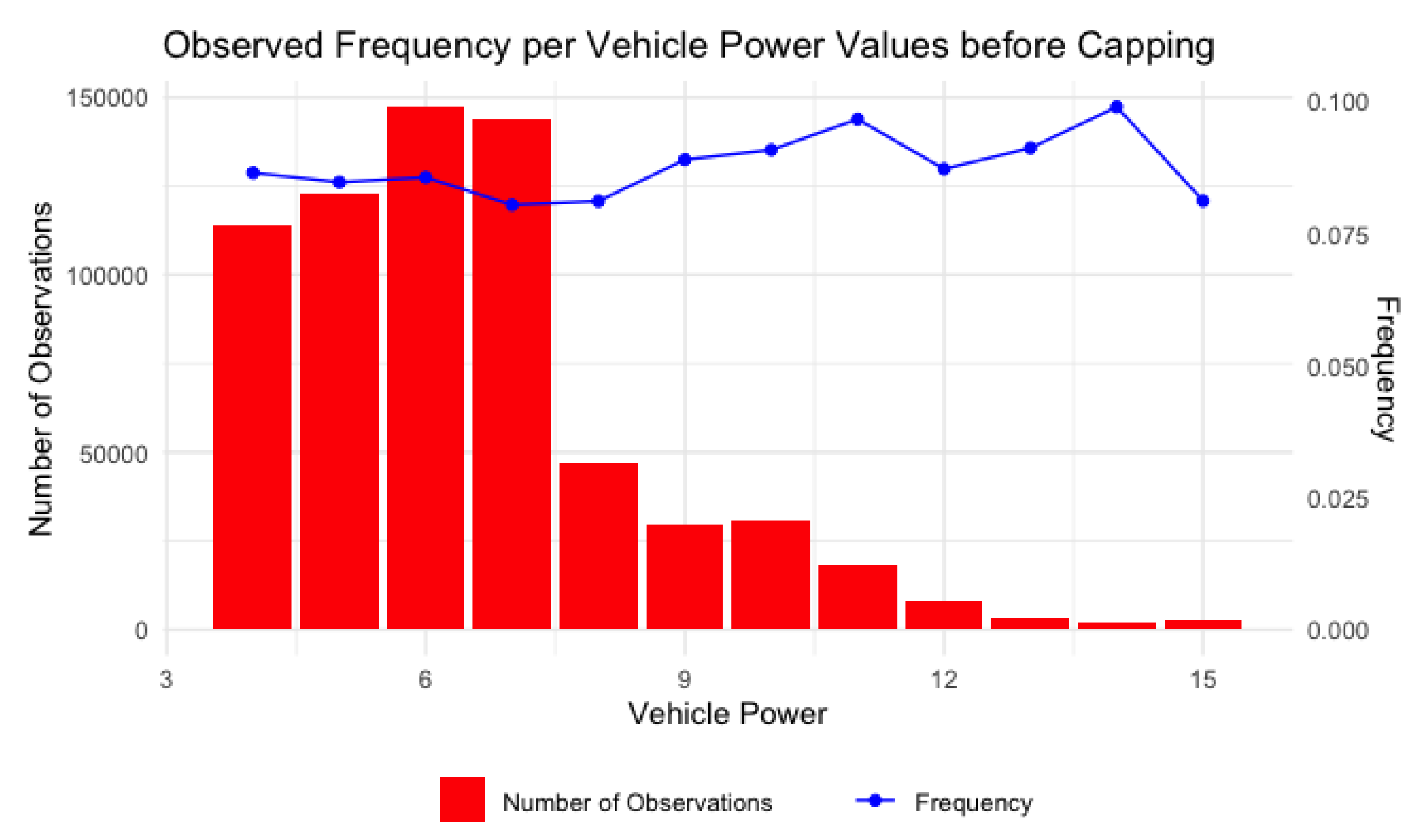
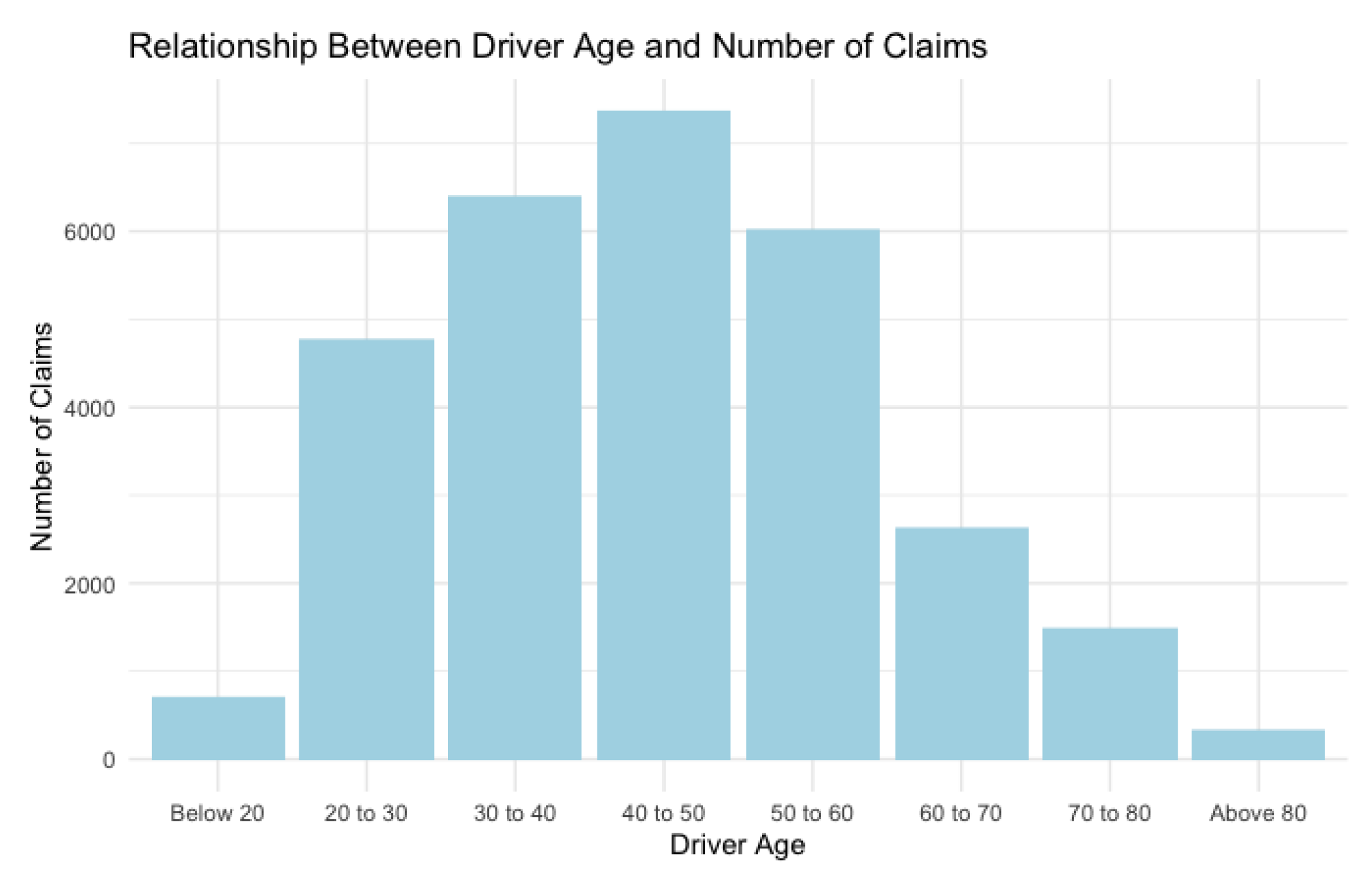
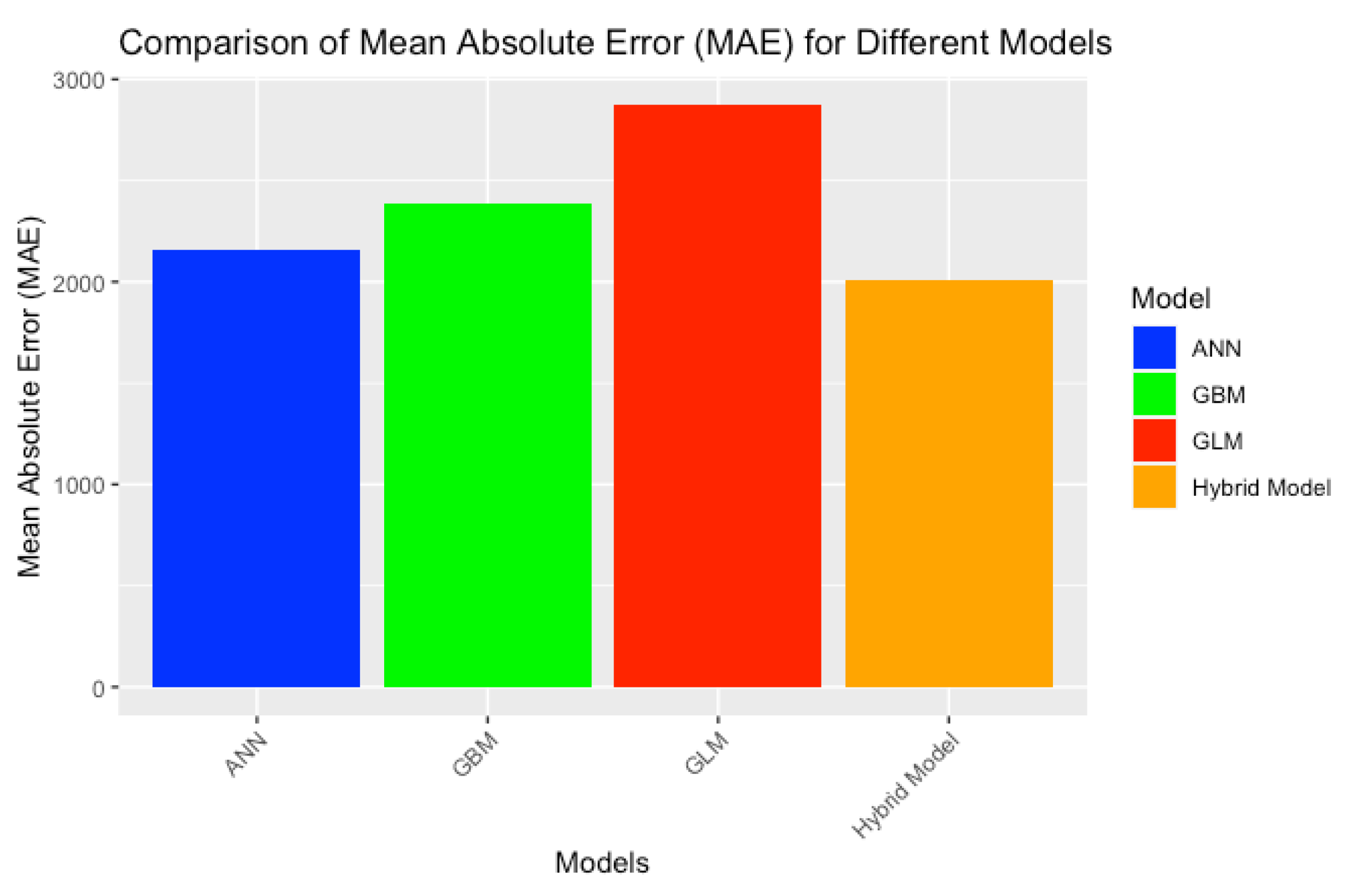
Table 1.
Features from the freMTLP2freq dataset.
| Feature | Description | Data Type |
|---|---|---|
| IDpol | The policy ID (can be linked with severity dataset) | Number |
| ClaimNb | Number of claims during the given period | Integer |
| Exposure | The exposure period for the policy | Number |
| Area | Indicates the density value where the car driver lives; “A” for rural area to “F” for urban areas | Character |
| VehPower | Power of the vehicle | Integer |
| VehAge | Age of the vehicle, in years | Integer |
| DrivAge | The driver’s age, in years (in France, the legal driving age is 18) | Integer |
| BonusMalus | Bonus/Malus: This ranges from 50 to 350. In France, a score of 100 or less means Bonus, and above 100 means Malus | Integer |
| VehBrand | Vehicle brand | Character |
| VehGas | Gas for the car, either regular or diesel | Character |
| Density | The population density (measured as people per square kilometer) in the city where the car driver resides | Integer |
| Region | France’s policy region (based on a classification from 1970 to 2015) | Character |
Table 2.
Features from the freMTLP2sev dataset.
| Feature | Description | Data Type |
|---|---|---|
| IDpol | The policy ID (used to link to frequency data) | Number |
| ClaimAmount | Amounts associated with claims | Integer |
Table 3.
Hyperparameters obtained for the frequency model.
| Hyperparameters | Layer 1 | Layer 2 | Layer 3 |
|---|---|---|---|
| Number of Neurons | 64 | 80 | 88 |
| Activation Function | tanh | sigmoid | relu |
| Learning Rate | 0.01 | 0.01 | 0.01 |
Table 4.
Hyperparameters obtained for the severity model.
| Hyperparameters | Layer 1 | Layer 2 | Layer 3 | Layer 4 |
|---|---|---|---|---|
| Number of Neurons | 256 | 32 | 72 | 88 |
| Activation Function | sigmoid | tanh | tanh | tanh |
| Learning Rate | 0.01 | 0.01 | 0.01 | 0.01 |
Table 5.
MAE values for GLM, GBM, ANN, and hybrid models.
| Model | MAE Values (Uncapped Variables) | MAE Values (Capped Variables) |
|---|---|---|
| GLM | 2972.235 | 2870.645 |
| GBM | 2518.398 | 2390.457 |
| ANN | 3106.231 | 2153.827 |
| Hybrid model (ANN & GLM) | 3043.405 | 2011.907 |
Disclaimer/Publisher’s Note: The statements, opinions and data contained in all publications are solely those of the individual author(s) and contributor(s) and not of MDPI and/or the editor(s). MDPI and/or the editor(s) disclaim responsibility for any injury to people or property resulting from any ideas, methods, instructions or products referred to in the content. |
© 2024 by the authors. Licensee MDPI, Basel, Switzerland. This article is an open access article distributed under the terms and conditions of the Creative Commons Attribution (CC BY) license (https://creativecommons.org/licenses/by/4.0/).
Share and Cite
MDPI and ACS Style
Wilson, A.A.; Nehme, A.; Dhyani, A.; Mahbub, K. A Comparison of Generalised Linear Modelling with Machine Learning Approaches for Predicting Loss Cost in Motor Insurance. Risks 2024, 12, 62. https://doi.org/10.3390/risks12040062
AMA Style
Wilson AA, Nehme A, Dhyani A, Mahbub K. A Comparison of Generalised Linear Modelling with Machine Learning Approaches for Predicting Loss Cost in Motor Insurance. Risks. 2024; 12(4):62. https://doi.org/10.3390/risks12040062
Chicago/Turabian StyleWilson, Alinta Ann, Antonio Nehme, Alisha Dhyani, and Khaled Mahbub. 2024. "A Comparison of Generalised Linear Modelling with Machine Learning Approaches for Predicting Loss Cost in Motor Insurance" Risks 12, no. 4: 62. https://doi.org/10.3390/risks12040062
Note that from the first issue of 2016, this journal uses article numbers instead of page numbers. See further details here.