An Optimal Three-Way Stable and Monotonic Spectrum of Bounds on Quantiles: A Spectrum of Coherent Measures of Financial Risk and Economic Inequality

Abstract

A spectrum of upper bounds ${\left(Q_{\alpha }(X;p)\right)}_{\alpha \in [0,\infty ]}$ on the (largest) $(1-p)$-quantile $Q(X;p)$ of an arbitrary random variable X is introduced and shown to be stable and monotonic in α, p, and X, with $Q_0(X;p)=Q(X;p)$. If p is small enough and the distribution of X is regular enough, then $Q_{\alpha }(X;p)$ is rather close to $Q(X;p)$. Moreover, these quantile bounds are coherent measures of risk. Furthermore, $Q_{\alpha }(X;p)$ is the optimal value in a certain minimization problem, the minimizers in which are described in detail. This allows of a comparatively easy incorporation of these bounds into more specialized optimization problems. In finance, $Q_0(X;p)$ and $Q_1(X;p)$ are known as the value at risk (VaR) and the conditional value at risk (CVaR). The bounds $Q_{\alpha }(X;p)$ can also be used as measures of economic inequality. The spectrum parameter α plays the role of an index of sensitivity to risk. The problems of the effective computation of the bounds are considered. Various other related results are obtained.

1. Introduction

The most common measure of risk is apparently the value at risk, ${VaR}_p(X)$, defined as the largest $(1-p)$-quantile of (the distribution of) a random variable (r.v.) X, which represents an uncertain future loss on an investment portfolio. Whereas very simple conceptually, the risk measure ${VaR}_p$ is not subadditive and, hence, is not coherent, in the sense established by Artzner et al. [1] and widely accepted afterwards. Other flaws of the value at risk are also well known; quoting Rockafellar and Uryasev [2]:

A very serious shortcoming of VaR, in addition, is that it provides no handle on the extent of the losses that might be suffered beyond the threshold amount indicated by this measure. It is incapable of distinguishing between situations where losses that are worse may be deemed only a little bit worse, and those where they could well be overwhelming. Indeed, it merely provides a lowest bound for losses in the tail of the loss distribution and has a bias toward optimism instead of the conservatism that ought to prevail in risk management.

In other words, the $VaR$ is not sensitive to the amount of risk beyond the threshold. Moreover, as is also discussed in [2], ${VaR}_p(X)$ is unstable in p and unstable in (the distribution of) X: arbitrarily small changes of the confidence level $1-p$ or of the composition of the portfolio may effect arbitrarily large changes of the value of ${VaR}_p(X)$. Closely related to these two kinds of instability is the inherent instability in the computation of ${VaR}_p(X)$.

To address these deficiencies of the $VaR$, Rockafellar and Uryasev [2,3] proposed an alternative risk measure, $CVaR$, which stands for the conditional value at risk. In the case when (the distribution of) the r.v. X is continuous, ${CVaR}_p(X)$ can be defined as $\mathsf{E}(X|X⩾{VaR}_p(X))$, the conditional expectation of the loss given that the loss X exceeds the threshold ${VaR}_p(X)$. This alternative risk measure, ${CVaR}_p(X)$, is coherent and stable in p and in X; it also has a certain, fixed sensitivity to the losses beyond the threshold.

However, ${CVaR}_p(X)$ provides no handle on the degree of sensitivity to risk. In particular, as will be demonstrated in Section 5.2, one can easily construct two portfolios with the same value of ${CVaR}_p$, such that one of the portfolios is clearly riskier than the other. Such indifference may generally be considered “an unwanted characteristic”; see e.g. comments on pages 36 and 48 in [4].

The main objective of the present paper is to remedy this indifference and provide the mentioned missing handle on the degree of sensitivity to risk, while retaining the coherence and stability properties. Indeed, we shall present a spectrum of risk measures ${\left(Q_{\alpha }(X;p)\right)}_{\alpha \in [0,\infty ]}$, where the spectrum parameter α may be considered the degree of sensitivity to risk: the greater the value of α, the greater the sensitivity to risk; see Section 5.2 for details. In particular, $\alpha =\infty$ corresponds to an “exponentially” high degree of risk sensitivity. Moreover, the proposed spectrum of risk measures possesses the following properties:

(I)

The common risk measures $VaR$ and $CVaR$ are in the spectrum: $Q_0(X;p)={VaR}_p(X)$ and $Q_1(X;p)={CVaR}_p(X)$; thus, $Q_{\alpha }(X;p)$ interpolates between ${VaR}_p(X)$ and ${CVaR}_p(X)$ for $\alpha \in (0,1)$ and extrapolates from ${VaR}_p(X)$ and ${CVaR}_p(X)$ on towards higher degrees of risk sensitivity for $\alpha \in (1,\infty ]$. Details on this can be found in Section 5.1.

(II)

The risk measure $Q_{\alpha }(·;p)$ is coherent for each $\alpha \in [1,\infty ]$ and each $p\in (0,1)$, but it is not coherent for any $\alpha \in [0,1)$ and any $p\in (0,1)$. Thus, $\alpha =1$ is the smallest value of the sensitivity index for which the risk measure $Q_{\alpha }(X;p)$ is coherent. One may also say that for $\alpha \in [1,\infty ]$ the risk measure $Q_{\alpha }(·;p)$ inherits the coherence of ${CVaR}_p=Q_1(·;p)$, and for $\alpha \in [0,1)$ it inherits the lack of coherence of ${VaR}_p=Q_0(·;p)$. For details, see Section 5.3.

(III)

$Q_{\alpha }(X;p)$ is three-way stable and monotonic: in $\alpha \in (0,\infty ]$, in $p\in (0,1)$, and in X. Moreover, as stated in Theorem 3.4 and Proposition 3.5, $Q_{\alpha }(X;p)$ is nondecreasing in X with respect to the stochastic dominance of any order $\gamma \in [1,\alpha +1]$; but, this monotonicity property breaks down for the stochastic dominance of any order $\gamma \in (\alpha +1,\infty ]$. Thus, the sensitivity index α is in a one-to-one correspondence with the highest order of the stochastic dominance respected by $Q_{\alpha }(X;p)$.

Rockafellar and Uryasev [2] also wrote: “Most importantly for applications, however, CVaR can be expressed by a remarkable minimization formula.” It will be shown (in Theorem 3.3) that our risk measures $Q_{\alpha }(X;p)$ possess quite a similar variational representation for each $\alpha \in (0,\infty ]$, which in fact generalizes the minimization formula for $CVaR$. This representation allows of a comparatively easy incorporation of the risk measures $Q_{\alpha }(X;p)$ into more specialized optimization problems, with additional restrictions on the r.v. X; see Section 4.3 for details.

The spectrum of risk measures ${\left(Q_{\alpha }(X;p)\right)}_{\alpha \in [0,\infty ]}$ is naturally based on a previously developed spectrum ${\left(P_{\alpha }(X;x)\right)}_{\alpha \in [0,\infty ]}$ of upper bounds on the tail probability $\mathsf{P}(X⩾x)$ for $x\in \mathbb{R}$, with $P_0(X;x)=\mathsf{P}(X⩾x)$ and $P_{\infty }(X;x)$ being the best possible exponential upper bound on $\mathsf{P}(X⩾x)$; see, e.g., [5,6] and bibliography therein; a shorter version of [6] appeared as [7]. The spectrum ${\left(P_{\alpha }(X;x)\right)}_{\alpha \in [0,\infty ]}$ is shown in the present paper to be stable and monotonic in α, x, and X. The bounds $P_{\alpha }(X;x)$ are optimal values in certain minimization problems. It is shown that the mentioned minimization problems for which $P_{\alpha }(X;x)$ and $Q_{\alpha }(X;p)$ are the optimal values are in a certain sense dual to each other; in the special case $\alpha =\infty$, this corresponds to the bilinear Legendre–Fenchel duality.

A few related results are obtained as well. In particular, a generalization of the Cillo–Delquie necessary and sufficient condition for the so-called mean-risk (M-R) to be nondecreasing with respect to the stochastic dominance of order 1 is presented, with a short proof. Moreover, a necessary and sufficient condition for the M-R measure to be coherent is given.

It is also shown that the quantile bounds $Q_{\alpha }(X;p)$ can be used as measures of economic inequality, and then the spectrum parameter α may be considered an index of sensitivity to inequality: the greater is the value of α, the greater is the sensitivity of the function $Q_{\alpha }(·;p)$ to inequality.

In addition, it is demonstrated that $P_{\alpha }(X;x)$ and $Q_{\alpha }(X;p)$ can be effectively computed.

The paper is structured as follows.

*

In Section 2, the three-way stability and monotonicity, as well as other useful properties, of the spectrum ${\left(P_{\alpha }(X;x)\right)}_{\alpha \in [0,\infty ]}$ of upper bounds on tail probabilities are established.

*

In Section 3, the corresponding properties of the spectrum ${\left(Q_{\alpha }(X;p)\right)}_{\alpha \in [0,\infty ]}$ of risk measures are presented, as well as other useful properties.

*

The matters of effective computation of $P_{\alpha }(X;x)$ and $Q_{\alpha }(X;p)$, as well as optimization of $Q_{\alpha }(X;p)$ with respect to X, are considered in Section 4.

*

An extensive discussion of results is presented in Section 5, particularly in relation with existing literature.

*

Concluding remarks are collected in Section 6.

*

The necessary proofs are given in Appendix A.

Further details can be found in the arXiv version of this paper [8].

2. An Optimal Three-Way Stable and Three-Way Monotonic Spectrum of Upper Bounds on Tail Probabilities

Consider the family ${(h_{\alpha })}_{\alpha \in [0,\infty ]}$ of functions $h_{\alpha }:\mathbb{R}\to \mathbb{R}$ given by the formula

$$h_{\alpha }(u):=\left\{\begin{array}{cccc}& \mathsf{I}\{u⩾0\}\hfill & & \text{if}\alpha =0,\hfill \\ & {(1+u/\alpha )}_{+}^{\alpha }\hfill & & \text{if}0<\alpha <\infty ,\hfill \\ & e^u\hfill & & \text{if}\alpha =\infty \hfill \end{array}\right.$$

(2.1)

for all $u\in \mathbb{R}$. Here, as usual, $\mathsf{I}\{·\}$ denotes the indicator function, $u_{+}:=0\vee u$ and $u_{+}^{\alpha }:={(u_{+})}^{\alpha }$ for all real u.

Obviously, the function $h_{\alpha }$ is nonnegative and nondecreasing for each $\alpha \in [0,\infty ]$, and it is also continuous for each $\alpha \in (0,\infty ]$. Moreover, it is easy to see that, for each $u\in \mathbb{R}$,

$$h_{\alpha }(u)\text{is}\text{nondecreasing}\text{and}\text{continuous}\text{in}\alpha \in [0,\infty ].$$

(2.2)

Next, let us use the functions $h_{\alpha }$ as generalized moment functions and thus introduce the generalized moments

$$A_{\alpha }(X;x)(\lambda ):=\mathsf{E}{h}_{\alpha }\left(\lambda (X-x)\right).$$

(2.3)

Here and in what follows, unless otherwise specified, X is any random variable (r.v.), $x\in \mathbb{R}$, $\alpha \in [0,\infty ]$, and $\lambda \in (0,\infty )$. Since $h_{\alpha }⩾0$, the expectation in formula (2.3) is always defined, but may take the value ∞. It may be noted that in the particular case $\alpha =0$, one has

$$A_0(X;x)(\lambda )=\mathsf{P}(X⩾x),$$

(2.4)

which does not actually depend on $\lambda \in (0,\infty )$.

Now one can introduce the expressions

$$P_{\alpha }(X;x):=\underset{\lambda \in (0,\infty )}{inf}{A}_{\alpha }(X;x)(\lambda )=\left\{\begin{array}{cccc}& \mathsf{P}(X⩾x)\hfill & & \text{if}\alpha =0,\hfill \\ & \underset{\lambda \in (0,\infty )}{inf}{\mathsf{E}(1+\lambda (X-x)/\alpha )}_{+}^{\alpha }\hfill & & \text{if}0<\alpha <\infty ,\hfill \\ & \underset{\lambda \in (0,\infty )}{inf}\mathsf{E}{e}^{\lambda (X-x)}\hfill & & \text{if}\alpha =\infty .\hfill \end{array}\right.$$

(2.5)

By the property stated in (2.2), $A_{\alpha }(X;x)(\lambda )$ and $P_{\alpha }(X;x)$ are nondecreasing in $\alpha \in [0,\infty ]$. In particular,

$$P_0(X;x)=\mathsf{P}(X⩾x)⩽P_{\alpha }(X;x).$$

(2.6)

It will be shown later (see Proposition 2.3) that $P_{\alpha }(X;x)$ also largely inherits the property of $h_{\alpha }(u)$ of being continuous in $\alpha \in [0,\infty ]$.

The definition (2.5) can be rewritten as

$$P_{\alpha }(X;x)=\underset{t\in T_{\alpha }}{inf}{\tilde{A}}_{\alpha }(X;x)(t)$$

(2.7)

where

$$\begin{array}{cc}\hfill T_{\alpha }& :=\left\{\begin{array}{cccc}& \mathbb{R}\hfill & & \text{if}\alpha \in [0,\infty )\text{,}\hfill \\ & (0,\infty )\hfill & & \text{if}\alpha =\infty \hfill \end{array}\right.\hfill \end{array}$$

(2.8)

and

$$\begin{array}{cc}\hfill {\tilde{A}}_{\alpha }(X;x)(t)& :=\left\{\begin{array}{cccc}& \frac{\mathsf{E}{(X-t)}_{+}^{\alpha }}{{(x-t)}_{+}^{\alpha }}\hfill & & \text{if}\alpha \in [0,\infty ),\hfill \\ & \mathsf{E}{e}^{(X-x)/t}\hfill & & \text{if}\alpha =\infty .\hfill \end{array}\right.\hfill \end{array}$$

(2.9)

Here and subsequently, we also use the conventions $0^0:=0$ and $\frac{a}{0}:=\infty$ for all $a\in [0,\infty ]$. The alternative representation (2.7) of $P_{\alpha }(X;x)$ follows because (i) $A_{\alpha }(X;x)(\lambda )={\tilde{A}}_{\alpha }(X;x)(x-\frac{\alpha }{\lambda })$ for $\alpha \in (0,\infty )$; (ii) $A_{\infty }(X;x)(\lambda )={\tilde{A}}_{\infty }(X;x)(\frac{1}{\lambda })$; and (iii) $P_0(X;x)=\mathsf{P}(X⩾x)={inf}_{t\in (-\infty ,x)}\mathsf{P}(X>t)={inf}_{t\in (-\infty ,x)}{\tilde{A}}_0(X;x)(t)$.

In view of Formula (2.7), one can see (cf. Corollary 2.3 in [5]) that, for each $\alpha \in [0,\infty ]$, $P_{\alpha }(X;x)$ is the optimal (that is, least possible) upper bound on the tail probability $\mathsf{P}(X⩾x)$ given the generalized moments $\mathsf{E}{g}_{\alpha ;t}(X)$ for all $t\in T_{\alpha }$, where:

$$g_{\alpha ;t}(u):=\left\{\begin{array}{cccc}& {(u-t)}_{+}^{\alpha }\hfill & & \text{if}\alpha \in [0,\infty ),\hfill \\ & e^{u/t}\hfill & & \text{if}\alpha =\infty .\hfill \end{array}\right.$$

(2.10)

In fact (cf. e.g. Proposition 3.3 in [6]), the bound $P_{\alpha }(X;x)$ remains optimal given the larger class of generalized moments $\mathsf{E}g(X)$ for all functions $g\in {\mathcal{H}}^{\alpha }$, where

$${\mathcal{H}}^{\alpha }:=\left\{g\in {\mathbb{R}}^{\mathbb{R}}:g(u)={\int }_{\mathbb{R}}{g}_{\alpha ;t}(u)\mu (dt)\text{for}\text{some}\mu \in {\mathrm{M}}_{\alpha }\text{and}\text{all}u\in \mathbb{R}\right\},$$

(2.11)

${\mathrm{M}}_{\alpha }$ denotes the set of all nonnegative Borel measures on $T_{\alpha }$, and, as usual, ${\mathbb{R}}^{\mathbb{R}}$ stands for the set of all real-valued functions on $\mathbb{R}$. By Proposition 1(ii) in [9] and Proposition 3.4 in [6],

$$0⩽\alpha <\beta ⩽\infty \text{implies}{\mathcal{H}}^{\alpha }\supseteq {\mathcal{H}}^{\beta }.$$

(2.12)

This provides the other way to come to the mentioned conclusion that

$$P_{\alpha }(X;x)\text{is}\text{nondecreasing}\text{in}\alpha \in [0,\infty ].$$

(2.13)

By Proposition 1.1 in [10], the class ${\mathcal{H}}^{\alpha }$ of generalized moment functions can be characterized as follows in the case when α is a natural number: for any $g\in {\mathbb{R}}^{\mathbb{R}}$, one has $g\in {\mathcal{H}}^{\alpha }$ if and only if g has finite derivatives $g^{(0)}:=g,g^{(1)}:=g^{\prime },\cdots ,g^{(\alpha -1)}$ on $\mathbb{R}$, such that $g^{(\alpha -1)}$ is convex on $\mathbb{R}$ and ${lim}_{x\to -\infty }{g}^{(j)}(x)=0$ for $j=0,1,\cdots ,\alpha -1$. Moreover, by Proposition 3.4 in [6], $g\in {\mathcal{H}}^{\infty }$ if and only if g is infinitely differentiable on $\mathbb{R}$, and $g^{(j)}⩾0$ on $\mathbb{R}$ and ${lim}_{x\to -\infty }{g}^{(j)}(x)=0$ for all $j=0,1,\cdots$.

Thus, the greater the value of α, the narrower and easier to deal with is the class ${\mathcal{H}}^{\alpha }$ and the smoother are the functions comprising ${\mathcal{H}}^{\alpha }$. However, the greater the value of α, the farther away is the bound $P_{\alpha }(X;x)$ from the true tail probability $\mathsf{P}(X⩾x)$.

Of the bounds $P_{\alpha }(X;x)$, the loosest and easiest one to get is $P_{\infty }(X;x)$, the so-called exponential upper bound on the tail probability $\mathsf{P}(X⩾x)$. It is used very widely, in particular when X is the sum of independent r.v.’s $X_i$, in which case one can rely on the factorization $A_{\alpha }(X;x)(\lambda )=e^{-\lambda x}{\prod }_i\mathsf{E}{e}^{\lambda X_i}$. A bound very similar to $P_3(X;x)$ was introduced in [11] in the case when X the sum of independent bounded r.v.’s; see also [12,13,14]. For any $\alpha \in (0,\infty )$, the bound $P_{\alpha }(X;x)$ is a special case of a more general bound given in Corollary 2.3 in [5]; see also Theorem 2.5 in [5]. For some of the further developments in this direction, see [7] and the bibliography therein. The papers mentioned in this paragraph used the representation (2.7) of $P_{\alpha }(X;x)$, rather than the new representation (2.5). The new representation appears, not only of more unifying form, but also more convenient as far as such properties of $P_{\alpha }(X;x)$ as the monotonicity in α and the continuity in α and in X are concerned; cf. (2.2) and the proofs of Propositions 2.3 and 2.4; those proofs, as well as the proofs of most of the other statements in this paper, are given in Appendix A. Yet another advantage of the representation (2.5) is that, for $\alpha \in [1,\infty )$, the function $A_{\alpha }(X;x)(·)$ inherits the convexity property of $h_{\alpha }$, which facilitates the minimization of $A_{\alpha }(X;x)(\lambda )$ in $\lambda$, as needed to find $P_{\alpha }(X;x)$ by Formula (2.5); relevant details on the remaining “difficult case” $\alpha \in (0,1)$ can be found in Section 4.1.

On the other hand, the “old” representation (2.7) of $P_{\alpha }(X;x)$ is more instrumental in establishing the mentioned connection with the classes ${\mathcal{H}}^{\alpha }$ of generalized moment functions; in proving Part (iii) of Proposition 2.2; and in discovering and proving Theorem 3.3.

***

Some of the more elementary properties of $P_{\alpha }(X;x)$ are presented in

Proposition 2.1.

(i) 

$P_{\alpha }(X;x)$ is nonincreasing in $x\in \mathbb{R}$.

(ii) 

If $\alpha \in (0,\infty )$ and $\mathsf{E}{X}_{+}^{\alpha }=\infty$, then $P_{\alpha }(X;x)=\infty$ for all $x\in \mathbb{R}$.

(iii) 

If $\alpha =\infty$ and $\mathsf{E}{e}^{\lambda X}=\infty$ for all real $\lambda >0$, then $P_{\infty }(X;x)=\infty$ for all $x\in \mathbb{R}$.

(iv) 

If $\alpha \in (0,\infty )$ and $\mathsf{E}{X}_{+}^{\alpha }<\infty$, then $P_{\alpha }(X;x)\to 1$ as $x\to -\infty$ and $P_{\alpha }(X;x)\to 0$ as $x\to \infty$, so that $0⩽P_{\alpha }(X;x)⩽1$ for all $x\in \mathbb{R}$.

(v) 

If $\alpha =\infty$ and $\mathsf{E}{e}^{{\lambda }_{0}X}<\infty$ for some real ${\lambda }_0>0$, then $P_{\alpha }(X;x)\to 1$ as $x\to -\infty$ and $P_{\alpha }(X;x)\to 0$ as $x\to \infty$, so that $0⩽P_{\alpha }(X;x)⩽1$ for all $x\in \mathbb{R}$.

In view of Proposition 2.1, it will be henceforth assumed by default that the tail bounds $P_{\alpha }(X;x)$ – as well as the quantile bounds $Q_{\alpha }(X;p)$, to be introduced in Section 3, and also the corresponding expressions $A_{\alpha }(X;x)(\lambda )$, ${\tilde{A}}_{\alpha }(X;x)(t)$, and $B_{\alpha }(X;p)(t)$, as in Formulas (2.3), (2.9), and (3.9)) are defined and considered only for r.v.’s $X\in {\mathcal{X}}_{\alpha }$ (unless indicated otherwise), where

$${\mathcal{X}}_{\alpha }:=\left\{\begin{array}{cccc}& \mathcal{X}\hfill & & \text{if}\alpha =0,\hfill \\ & \left\{X\in \mathcal{X}:\mathsf{E}{X}_{+}^{\alpha }<\infty \right\}\hfill & & \text{if}\alpha \in (0,\infty ),\hfill \\ & \left\{X\in \mathcal{X}:{\Lambda }_X\ne \mathsf{Ø}\right\}\hfill & & \text{if}\alpha =\infty ,\hfill \end{array}\right.$$

(2.14)

$\mathcal{X}$ is the set of all real-valued r.v.’s on a given probability space (implicit in this paper), and

$${\Lambda }_X:=\left\{\lambda \in (0,\infty ):\mathsf{E}{e}^{\lambda X}<\infty \right\}.$$

(2.15)

Observe that the set ${\mathcal{X}}_{\alpha }$ is a convex cone containing all real constants; for details on this, one may see comments in the paragraph containing Formula (1.14) in [8].

As usual, we let ${\parallel Z\parallel }_{\alpha }:={(\mathsf{E}|Z|}^{\alpha }{)}^{1/\alpha }$, the ${\mathcal{L}}^{\alpha }$-norm of a r.v. Z, which is actually a norm if and only if $\alpha ⩾1$.

It follows from Proposition 2.1 and Formula (2.6) that

$$P_{\alpha }(X;x)\text{is}\text{nonincreasing}\text{in}x\in \mathbb{R}\text{,}\text{with}{P}_{\alpha }(X;(-\infty )+)=1\text{and}{P}_{\alpha }(X;\infty -)=0\text{.}$$

(2.16)

Here, as usual, $f(a+)$ and $f(a-)$ denote the right and left limits of f at a.

One can say more in this respect. To do that, introduce

$$x_{*}:=x_{*,X}:=supsuppX\text{and}{p}_{*}:=p_{*,X}:=\mathsf{P}(X=x_{*}).$$

(2.17)

Here, as usual, $suppX$ denotes the support set of (the distribution of the r.v.) X; speaking somewhat loosely, $x_{*}$ is the maximum value taken by the r.v. X, and $p_{*}$ is the probability with which this value is taken. It is of course possible that $x_{*}=\infty$, in which case necessarily $p_{*}=0$, since the r.v. X was assumed to be real-valued.

Introduce also

$$x_{\alpha }:=x_{\alpha ,X}:=inf{E}_{\alpha }(1),$$

(2.18)

where

$$E_{\alpha }(p):=E_{\alpha ,X}(p):=\{x\in \mathbb{R}:P_{\alpha }(X;x)<p\}.$$

(2.19)

Recall that, according to the standard convention, for any subset E of $\mathbb{R}$, $infE=\infty$ if and only if $E=\mathsf{Ø}$. Now, one can state

Proposition 2.2. 

(i) 

For all $x\in [x_{*},\infty )$, one has $P_{\alpha }(X;x)=P_0(X;x)=\mathsf{P}(X⩾x)=\mathsf{P}(X=x)=p_{*}\mathsf{I}\{x=x_{*}\}.$ 

(ii) 

For all $x\in (-\infty ,x_{*})$, one has $P_{\alpha }(X;x)>0$.

(iii) 

The function $(-\infty ,x_{*}]\cap \mathbb{R}\ni x\mapsto P_{\alpha }{(X;x)}^{-1/\alpha }$ is continuous and convex if $\alpha \in (0,\infty )$; we use the conventions $0^{-a}:=\infty$ and ${\infty }^{-a}:=0$ for all real $a>0$; concerning the continuity of functions with values in the set $[0,\infty ]$, we use the natural topology on this set. Also, the function $(-\infty ,x_{*}]\cap \mathbb{R}\ni x\mapsto -ln{P}_{\infty }(X;x)$ is continuous and convex, with the convention $ln0:=-\infty$.

(iv) 

If $\alpha \in (0,\infty ]$, then the function $(-\infty ,x_{*}]\cap \mathbb{R}\ni x\mapsto P_{\alpha }(X;x)$ is continuous.

(v) 

The function $\mathbb{R}\ni x\mapsto P_{\alpha }(X;x)$ is left-continuous.

(vi) 

$x_{\alpha }$ is nondecreasing in $\alpha \in [0,\infty ]$, and $x_{\alpha }<\infty$ for all $\alpha \in [0,\infty ]$.

(vii) 

If $\alpha \in [1,\infty ]$, then $x_{\alpha }=\mathsf{E}X$; even for $X\in {\mathcal{X}}_{\alpha }$, it is of course possible that $\mathsf{E}X=-\infty$, in which case $P_{\alpha }(X;x)<1$ for all real x.

(viii) 

$x_{\alpha }⩽x_{*}$, and $x_{\alpha }=x_{*}$ if and only if $p_{*}=1$.

(ix) 

$E_{\alpha }(1)=(x_{\alpha },\infty )\ne \mathsf{Ø}$.

(x) 

$P_{\alpha }(X;x)=1$ for all $x\in (-\infty ,x_{\alpha }]$.

(xi) 

If $\alpha \in (0,\infty ]$, then $P_{\alpha }(X;x)$ is strictly decreasing in $x\in [x_{\alpha },x_{*}]\cap \mathbb{R}$.

This proposition will be useful when establishing continuity properties of the quantile bounds considered in Section 3 and the matters of effective computation addressed in Section 4. Moreover, Proposition 2.2 will be heavily used in the proof of Proposition 3.1 to establish basic properties of the risk measures $Q_{\alpha }(X;p)$.

For $\alpha \in (1,\infty )$, Parts (i), (iv), (vii), (x), and (xi) of Proposition 2.2 are contained in [6], Proposition 3.2.

One may also note here that, by (2.16) and Part (v) of Proposition 2.2, the function $P_{\alpha }(X;·)$ may be regarded as the tail function of some r.v. $Z_{\alpha }$: $P_{\alpha }(X;u)=\mathsf{P}(Z_{\alpha }⩾u)$ for all real u.

Some parts of Propositions 2.1 and 2.2 are illustrated in Example 1.3 in [8] and in the corresponding figure there.

Proposition 2.3. $P_{\alpha }(X;x)$ is continuous in $\alpha \in [0,\infty ]$ in the following sense: Suppose that $({\alpha }_n)$ is any sequence in $[0,\infty )$ converging to $\alpha \in [0,\infty ]$, with $\beta :={sup}_n{\alpha }_n$ and $X\in {\mathcal{X}}_{\beta }$; then $P_{{\alpha }_n}(X;x)\to P_{\alpha }(X;x)$.

In view of Parts (ii) and (iii) of Proposition 2.1, the condition $X\in {\mathcal{X}}_{\beta }$ in Proposition 2.3 is essential.

Let us now turn to the question of stability of $P_{\alpha }(X;x)$ with respect to (the distribution of) X. First here, recall that one of a number of mutually equivalent definitions of the convergence in distribution, $X_n\underset{n\to \infty }{\stackrel{\mathrm{D}}{⟶}}X$, of a sequence of r.v.’s $X_n$ to an r.v. X is the following: $\mathsf{P}(X_n⩾x)\underset{n\to \infty }{⟶}\mathsf{P}(X⩾x)$ for all real x such that $\mathsf{P}(X=x)=0$; cf.; cf. e.g. [15, §4 and Theorem 2.1].

We shall also need the following uniform integrability condition:

$$\begin{array}{cc}& \underset{n}{sup}\mathsf{E}{(X_n)}_{+}^{\alpha }\mathsf{I}\{X_n>N\}\underset{N\to \infty }{⟶}0\text{if}\alpha \in (0,\infty )\text{,}\hfill \end{array}$$

(2.20)

$$\begin{array}{cc}& \underset{n}{sup}\mathsf{E}{e}^{\lambda X_n}\mathsf{I}\{X_n>N\}\underset{N\to \infty }{⟶}0\text{for}\text{each}\lambda \in {\Lambda }_X\text{if}\alpha =\infty .\hfill \end{array}$$

(2.21)

Proposition 2.4. Suppose that $\alpha \in (0,\infty ]$. Then $P_{\alpha }(X;x)$ is continuous in X in the following sense. Take any sequence ${(X_n)}_{n\in \mathbb{N}}$ of real-valued r.v.’s such that $X_n\underset{n\to \infty }{\stackrel{\mathrm{D}}{⟶}}X$ and the uniform integrability condition (2.20)- (2.21) is satisfied. Then one has the following.

(i) 

The convergence

$$P_{\alpha }(X_n;x)\underset{n\to \infty }{⟶}{P}_{\alpha }(X;x)$$

(2.22)

takes place for all real $x\ne x_{*}$, where $x_{*}=x_{*,X}$ as in (2.17); thus, by Parts (i) and (iv) of Proposition 2.2, (2.22) holds for all real x that are points of continuity of the function $P_{\alpha }(X;·)$.

(ii) 

The convergence (2.22) holds for $x=x_{*}$ as well, provided that $\mathsf{P}(X_n=x_{*})\underset{n\to \infty }{⟶}\mathsf{P}(X=x_{*})$. In particular, (2.22) holds for $x=x_{*}$ if $\mathsf{P}(X=x_{*})=0$.

Note that in the case $\alpha =0$ the convergence (2.22) may fail to hold, not only for $x=x_{*}$, but for all real x such that $\mathsf{P}(X=x)>0$.

***

Let us now discuss matters of monotonicity of $P_{\alpha }(X;x)$ in X, with respect to various orders on the mentioned set $\mathcal{X}$ of all real-valued r.v.’s X. Using the family of function classes ${\mathcal{H}}^{\alpha }$, defined by (2.11), one can introduce a family of stochastic orders, say $\stackrel{\alpha +1}{⩽}$, on the set $\mathcal{X}$ by the formula

$$X\stackrel{\alpha +1}{⩽}Y\stackrel{\text{def}}{\iff }\mathsf{E}g(X)⩽\mathsf{E}g(Y)\text{for}\text{all}g\in {\mathcal{H}}^{\alpha },$$

where $\alpha \in [0,\infty ]$ and X and Y are in $\mathcal{X}$. To avoid using the term “order” with two different meanings in one phrase, let us refer to the relation $\stackrel{\alpha +1}{⩽}$ as the stochastic dominance of order $\alpha +1$, rather than the stochastic order of order $\alpha +1$. In view of (2.11), it is clear that

$$X\stackrel{\alpha +1}{⩽}Y\iff \mathsf{E}{g}_{\alpha ;t}(X)⩽\mathsf{E}{g}_{\alpha ;t}(Y)\text{for}\text{all}t\in T_{\alpha },$$

(2.23)

so that, in the case when $\alpha =m-1$ for some natural number m, the order $\stackrel{\alpha +1}{⩽}$ coincides with the “m-increasing-convex” order ${⩽}_{m-\text{icx}}$ as defined e.g. on page 206 in [16]. In particular,

$$\begin{array}{cc}\hfill X\stackrel{1}{⩽}Y& \iff \mathsf{P}(X>t)⩽\mathsf{P}(Y>t)\text{for}\text{all}t\in \mathbb{R}\hfill \\ & \iff \mathsf{P}(X⩾t)⩽\mathsf{P}(Y⩾t)\text{for}\text{all}t\in \mathbb{R}\iff X\stackrel{\mathrm{st}}{⩽}Y,\hfill \end{array}$$

(2.24)

where $\stackrel{\mathrm{st}}{⩽}$ denotes the usual stochastic dominance of order 1, and:

$$\begin{array}{cc}\hfill X\stackrel{2}{⩽}Y& \iff \mathsf{E}{(X-t)}_{+}⩽\mathsf{E}{(Y-t)}_{+}\text{for}\text{all}t\in \mathbb{R},\hfill \end{array}$$

(2.25)

so that $\stackrel{2}{⩽}$ coincides with the usual stochastic dominance of order 2. Also,

$$X\stackrel{\mathrm{st}}{⩽}Y\text{iff}\text{for}\text{some}\text{r.v.’s}{X}_1\text{and}{Y}_1\text{one}\text{has}{X}_1⩽Y_1\text{,}{X}_1\stackrel{\mathrm{D}}{=}X\text{,}\text{and}{Y}_1\stackrel{\mathrm{D}}{=}Y\text{,}$$

(2.26)

where $\stackrel{\mathrm{D}}{=}$ denotes the equality in distribution.

By (2.12), the orders $\stackrel{\alpha +1}{⩽}$ are graded in the sense that

$$\text{if}X\stackrel{\alpha +1}{⩽}Y\text{for}\text{some}\alpha \in [0,\infty ]\text{,}\text{then}X\stackrel{\beta +1}{⩽}Y\text{for}\text{all}\beta \in [\alpha ,\infty ]\text{.}$$

(2.27)

A stochastic order, which is a “mirror image” of the order $\stackrel{\alpha +1}{⩽}$, but only for nonnegative r.v.’s, was presented by Fishburn in [17]; note Theorem 2 in [17] on the relation with a “bounded” version of this order, previously introduced and studied in [18]. Denoting the corresponding Fishburn [17] order by ${⩽}_{\alpha +1}$, one has

$$X{⩽}_{\alpha +1}Y\iff (-Y)\stackrel{\alpha +1}{⩽}(-X),$$

(2.28)

for nonnegative r.v.’s X and Y. However, as shown in this paper (recall Proposition 2.1), the condition of the nonnegativity of the r.v.’s is not essential; without it, one can either deal with infinite expected values or, alternatively, require that they be finite. The case when α is an integer was considered, in a different form, in [19].

One may also consider the order ${⩽}_{\alpha }^{-1}$ defined by the condition that $X{⩽}_{\alpha }^{-1}Y$ if and only if X and Y are nonnegative r.v.’s and $F_X^{(-\alpha )}(p)⩽F_Y^{(-\alpha )}(p)$ for all $p\in (0,1)$, where $\alpha \in (0,\infty )$,

$$\begin{array}{cc}\hfill F_X^{(-\alpha )}(p)& :=\frac{1}{\Gamma (\alpha )}{\int }_{[0,p)}{(p-u)}^{\alpha -1}d{F}_X^{-1}(u),\hfill \end{array}$$

(2.29)

$$\begin{array}{cc}\hfill F_X^{-1}(p)& :=inf\{x\in [0,\infty ):\mathsf{P}(X⩽x)⩾p\}=-Q(-X;p)\hfill \end{array}$$

(2.30)

with $Q(·;·)$ as in (3.3), and the integral in (2.29) is understood as the Lebesgue integral with respect to the nonnegative Borel measure ${\mu }_X^{-1}$ on $[0,1)$ defined by the condition that ${\mu }_X^{-1}\left([0,p)\right)=F_X^{-1}(p)$ for all $p\in (0,1)$; cf. [20,21]. Note that $F_X^{(-1)}(p)=F_X^{-1}(p)$. For nonnegative r.v.’s, the order ${⩽}_{\alpha +1}^{-1}$ coincides with the order ${⩽}_{\alpha +1}$ if $\alpha \in \{0,1\}$; again see [20,21]. Even for nonnegative r.v.’s, it seems unclear how the orders ${⩽}_{\alpha +1}$ and ${⩽}_{\alpha +1}^{-1}$ relate to each other for positive real $\alpha \ne 1$; see e.g. the discussion following Proposition 1 in [20] and Note ${}^1$ on page 100 in [22].

The following theorem summarizes some of the properties of the tail probability bounds $P_{\alpha }(X;x)$ established above and also adds a few simple properties of these bounds.

Theorem 2.5. The following properties of the tail probability bounds $P_{\alpha }(X;x)$ are valid.

Model-independence: 

$P_{\alpha }(X;x)$ depends on the r.v. X only through the distribution of X.

Monotonicity in X:

$P_{\alpha }(·;x)$ is nondecreasing with respect to the stochastic dominance of order $\alpha +1$: for any r.v. Y such that $X\stackrel{\alpha +1}{⩽}Y$, one has $P_{\alpha }(X;x)⩽P_{\alpha }(Y;x)$. Therefore, $P_{\alpha }(·;x)$ is nondecreasing with respect to the stochastic dominance of any order $\gamma \in [1,\alpha +1]$; in particular, for any r.v. Y such that $X⩽Y$, one has $P_{\alpha }(X;x)⩽P_{\alpha }(Y;x)$.

Monotonicity in α:

$P_{\alpha }(X;x)$ is nondecreasing in $\alpha \in [0,\infty ]$.

Monotonicity in x:

$P_{\alpha }(X;x)$ is nonincreasing in $x\in \mathbb{R}$.

Values: 

$P_{\alpha }(X;x)$ takes only values in the interval $[0,1]$.

α-concavity in x:

$P_{\alpha }{(X;x)}^{-1/\alpha }$ is convex in x if $\alpha \in (0,\infty )$, and $ln{P}_{\alpha }(X;x)$ is concave in x if $\alpha =\infty$.

Stability in x:

$P_{\alpha }(X;x)$ is continuous in x at any point $x\in \mathbb{R}$ – except the point $x=x_{*}$ when $p_{*}>0$.

Stability in α:

Suppose that a sequence $({\alpha }_n)$ is as in Proposition 2.3. Then $P_{{\alpha }_n}(X;x)\to P_{\alpha }(X;x)$.

Stability in X:

Suppose that $\alpha \in (0,\infty ]$ and a sequence $(X_n)$ is as in Proposition 2.4. Then $P_{\alpha }(X_n;x)\to P_{\alpha }(X;x)$.

Translation invariance: 

$P_{\alpha }(X+c;x+c)=P_{\alpha }(X;x)$ for all real c.

Consistency: 

$P_{\alpha }(c;x)=P_0(c;x)=\mathsf{I}\{c⩾x\}$ for all real c; that is, if the r.v. X is the constant c, then all the tail probability bounds $P_{\alpha }(X;x)$ precisely equal the true tail probability $\mathsf{P}(X⩾x)$.

Positive homogeneity: 

$P_{\alpha }(\kappa X;\kappa x)=P_{\alpha }(X;x)$ for all real $\kappa >0$.

3. An Optimal Three-Way Stable and Three-Way Monotonic Spectrum of Upper Bounds on Quantiles

Take any

$$p\in (0,1)$$

(3.1)

and introduce the generalized inverse (with respect to x) of the bound $P_{\alpha }(X;x)$ by the formula

$$Q_{\alpha }(X;p):=inf{E}_{\alpha ,X}(p)=inf\left\{x\in \mathbb{R}:P_{\alpha }(X;x)<p\right\},$$

(3.2)

where $E_{\alpha ,X}(p)$ is as in (2.19). In particular, in view of the equality in (2.6),

$$Q(X;p):=Q_0(X;p)=inf\left\{x\in \mathbb{R}:\mathsf{P}(X⩾x)<p\right\}=inf\left\{x\in \mathbb{R}:\mathsf{P}(X>x)<p\right\},$$

(3.3)

which is a $(1-p)$-quantile of (the distribution of) the r.v. X; actually, $Q(X;p)$ is the largest one in the set of all $(1-p)$-quantiles of X.

It follows immediately from (3.2), (2.13), and (3.3) that

$$\begin{array}{cc}& Q_{\alpha }(X;p)\text{is}\text{an}\text{upper}\text{bound}\text{on}\text{the}\text{quantile}Q(X;p)\text{,}\text{and}\hfill \\ & Q_{\alpha }(X;p)\text{is}\text{nondecreasing}\text{in}\alpha \in [0,\infty ]\text{.}\hfill \end{array}$$

(3.4)

Thus, one has a monotonic spectrum of upper bounds, $Q_{\alpha }(X;p)$, on the quantile $Q(X;p)$, ranging from the tightest bound, $Q_0(X;p)=Q(X;p)$, to the loosest one, $Q_{\infty }(X;p)$, which latter is based on the exponential bound $P_{\infty }(X;x)={inf}_{\lambda >0}\mathsf{E}{e}^{\lambda (X-x)}$ on $\mathsf{P}(X⩾x)$.

Also, it is obvious from (3.2) that

$$Q_{\alpha }(X;p)\text{is}\text{nonincreasing}\text{in}p\in (0,1)\text{.}$$

(3.5)

Basic properties of $Q_{\alpha }(X;p)$ are collected in

Proposition 3.1. Recall the definitions of $x_{*}$ and $x_{\alpha }$ in (2.17) and (2.18). The following statements are true.

(i) 

$Q_{\alpha }(X;p)\in \mathbb{R}$.

(ii) 

If $p\in (0,p_{*}]\cap (0,1)$ then $Q_{\alpha }(X;p)=x_{*}$.

(iii) 

$Q_{\alpha }(X;p)⩽x_{*}$.

(iv) 

$Q_{\alpha }(X;p)\underset{p\downarrow 0}{⟶}{x}_{*}$.

Figure 1. Illustration of Proposition 3.1

Figure 1. Illustration of Proposition 3.1

(v) 

If $\alpha \in (0,\infty ]$, then the function

$$(p_{*},1)\ni p\mapsto Q_{\alpha }(X;p)\in (x_{\alpha },x_{*})$$

(3.6)

is the unique inverse to the continuous strictly decreasing function

$$(x_{\alpha },x_{*})\ni x\mapsto P_{\alpha }(X;x)\in (p_{*},1).$$

(3.7)

Therefore, the function (3.6), too, is continuous and strictly decreasing.

(vi) 

If $\alpha \in (0,\infty ]$, then for any $y\in \left(-\infty ,Q_{\alpha }(X;p)\right)$, one has $P_{\alpha }(X;y)>p$.

(vii) 

If $\alpha \in [1,\infty ]$, then $Q_{\alpha }(X;p)>\mathsf{E}X$.

Example 3.2. Some parts of Proposition 3.1 are illustrated in Figure 1, with graphs $\{\left(p,Q_{\alpha }(X;p)\right):0<p<1\}$ in the important case when the r.v. X takes only two values. Then, by the translation invariance property stated below in Theorem 2.5, without loss of generality (w.l.o.g.) $\mathsf{E}X=0$. Thus, $X=X_{a,b}$, where a and b are positive real numbers and $X_{a,b}$ is a r.v. with the uniquely determined zero-mean distribution on the set $\{-a,b\}$. Let us take $a=1$ and $b=3$, with the values of α equal 0 (black), $\frac{1}{2}$ (blue), 1 (green), 2 (orange), and ∞ (red). One may compare this picture with the one for $P_{\alpha }(X;x)$ in Example 1.3 in [8] (where the same values of a, b, and α were used), having in mind that the function $Q_{\alpha }(X;·)$ is a generalized inverse to the function $P_{\alpha }(X;·)$.

The definition (3.2) of $Q_{\alpha }(X;p)$ is rather complicated, in view of the definition (2.5) of $P_{\alpha }(X;x)$. So, the following theorem will be useful, as it provides a more direct expression of $Q_{\alpha }(X;p)$; at that, one may again recall (3.3), concerning the case $\alpha =0$.

Theorem 3.3. For all $\alpha \in (0,\infty ]$

$$Q_{\alpha }(X;p)=\underset{t\in T_{\alpha }}{inf}{B}_{\alpha }(X;p)(t),$$

(3.8)

where $T_{\alpha }$ is as in (2.8) and

$$B_{\alpha }(X;p)(t):=\left\{\begin{array}{cccc}& t+\frac{{\parallel (X-t)}_{+}{\parallel }_{\alpha }}{p^{1/\alpha }}\hfill & & \text{for}\alpha \in (0,\infty )\text{,}\hfill \\ & tln\frac{\mathsf{E}{e}^{X/t}}{p}\hfill & & \text{for}\alpha =\infty \text{.}\hfill \end{array}\right.$$

(3.9)

Proof of Theorem 3.3. The proof is based on the simple observation, following immediately from the definitions (2.9) and (3.9), that the dual level sets for the functions ${\tilde{A}}_{\alpha }(X;x)$ and $B_{\alpha }(X;p)$ are the same:

$$T_{{\tilde{A}}_{\alpha }(X;x)}(p)=T_{B_{\alpha }(X;p)}(x)$$

(3.10)

for all $\alpha \in (0,\infty ]$, $x\in \mathbb{R}$, and $p\in (0,1)$, where

$$\begin{array}{cc}\hfill T_{{\tilde{A}}_{\alpha }(X;x)}(p)& :=\{t\in T_{\alpha }:{\tilde{A}}_{\alpha }(X;x)(t)<p\}\text{and}\hfill \\ \hfill T_{B_{\alpha }(X;p)}(x)& :=\{t\in T_{\alpha }:B_{\alpha }(X;p)(t)<x\}.\hfill \end{array}$$

Indeed, by (2.7) and (3.10),

$$\begin{array}{cc}& P_{\alpha }(X;x)<p\iff \underset{t\in T_{\alpha }}{inf}{\tilde{A}}_{\alpha }(X;x)(t)<p\hfill \\ & \iff T_{{\tilde{A}}_{\alpha }(X;x)}(p)\ne \mathsf{Ø}\iff T_{B_{\alpha }(X;p)}(x)\ne \mathsf{Ø}\hfill & \hfill \iff x>\underset{t\in T_{\alpha }}{inf}{B}_{\alpha }(X;p)(t).\end{array}$$

Now, (3.8) follows immediately by (3.2). ☐

Note that the case $\alpha =\infty$ of Theorem 3.3 is a special case of Proposition 1.5 in [23], and the above proof of Theorem 3.3 is similar to that of Proposition 1.5 in [23]. Correspondingly, the duality presented in the above proof of Theorem 3.3 is a generalization of the bilinear Legendre–Fenchel duality considered in [23].

The following theorem presents the most important properties of the quantile bounds $Q_{\alpha }(X;p)$, in addition to the variational representation of $Q_{\alpha }(X;p)$ given by Theorem 3.3.

Theorem 3.4. The following properties of the quantile bounds $Q_{\alpha }(X;p)$ are valid.

Model-independence: 

$Q_{\alpha }(X;p)$ depends on the r.v. X only through the distribution of X.

Monotonicity in X:

$Q_{\alpha }(·;p)$ is nondecreasing with respect to the stochastic dominance of order $\alpha +1$: for any r.v. Y such that $X\stackrel{\alpha +1}{⩽}Y$, one has $Q_{\alpha }(X;p)⩽Q_{\alpha }(Y;p)$. Therefore, $Q_{\alpha }(·;p)$ is nondecreasing with respect to the stochastic dominance of any order $\gamma \in [1,\alpha +1]$; in particular, for any r.v. Y such that $X⩽Y$, one has $Q_{\alpha }(X;p)⩽Q_{\alpha }(Y;p)$.

Monotonicity in α:

$Q_{\alpha }(X;p)$ is nondecreasing in $\alpha \in [0,\infty ]$.

Monotonicity in p:

$Q_{\alpha }(X;p)$ is nonincreasing in $p\in (0,1)$, and $Q_{\alpha }(X;p)$ is strictly decreasing in $p\in [p_{*},1)\cap (0,1)$ if $\alpha \in (0,\infty ]$.

Finiteness: 

$Q_{\alpha }(X;p)$ takes only (finite) real values.

Concavity in $p^{-1/\alpha }$ or in $ln\frac{1}{p}$: 

$Q_{\alpha }(X;p)$ is concave in $p^{-1/\alpha }$ if $\alpha \in (0,\infty )$, and $Q_{\infty }(X;p)$ is concave in $ln\frac{1}{p}$.

Stability in p:

$Q_{\alpha }(X;p)$ is continuous in $p\in (0,1)$ if $\alpha \in (0,\infty ]$.

Stability in X:

Suppose that $\alpha \in (0,\infty ]$ and a sequence $(X_n)$ is as in Proposition 2.4. Then $Q_{\alpha }(X_n;p)\to Q_{\alpha }(X;p)$.

Stability in α:

Suppose that $\alpha \in (0,\infty ]$ and a sequence $({\alpha }_n)$ is as in Proposition 2.3. Then $Q_{{\alpha }_n}(X;p)\to Q_{\alpha }(X;p)$.

Translation invariance: 

$Q_{\alpha }(X+c;p)=Q_{\alpha }(X;p)+c$ for all real c.

Consistency: 

$Q_{\alpha }(c;p)=c$ for all real c; that is, if the r.v. X is the constant c, then all of the quantile bounds $Q_{\alpha }(X;p)$ equal c.

Positive sensitivity: 

Suppose here that $X⩾0$. If at that $\mathsf{P}(X>0)>0$, then $Q_{\alpha }(X;p)>0$ for all $\alpha \in (0,\infty ]$; if, moreover, $\mathsf{P}(X>0)>p$, then $Q_0(X;p)>0$.

Positive homogeneity: 

$Q_{\alpha }(\kappa X;p)=\kappa Q_{\alpha }(X;p)$ for all real $\kappa ⩾0$.

Subadditivity: 

$Q_{\alpha }(X;p)$ is subadditive in X if $\alpha \in [1,\infty ]$; that is, for any other r.v. Y (defined on the same probability space as X) one has:

$$Q_{\alpha }(X+Y;p)⩽Q_{\alpha }(X;p)+Q_{\alpha }(Y;p).$$

Convexity: 

$Q_{\alpha }(X;p)$ is convex in X if $\alpha \in [1,\infty ]$; that is, for any other r.v. Y (defined on the same probability space as X) and any $t\in (0,1)$ one has

$$Q_{\alpha }\left((1-t)X+tY;p\right)⩽(1-t)Q_{\alpha }(X;p)+t{Q}_{\alpha }(Y;p)$$

The inequality $Q_1(X;p)⩽Q_{\infty }(X;p)$, in other notations, was mentioned (without proof) in [24]; of course, this inequality is a particular, and important, case of the monotonicity of $Q_{\alpha }(X;p)$ in $\alpha \in [0,\infty ]$. That $Q_{\alpha }(·;p)$ is nondecreasing with respect to the stochastic dominance of order $\alpha +1$ was shown (using other notations) in [25] in the case $\alpha =1$.

The following two propositions complement the monotonicity property of $Q_{\alpha }(X;p)$ in X stated in Theorem 3.4.

Proposition 3.5. The upper bound $\alpha +1$ on γ in the statement of the monotonicity of $Q_{\alpha }(X;p)$ in X in Theorem 3.4 is exact in the following rather strong sense. For any $\alpha \in [0,\infty )$, there exist r.v.’s X and Y in ${\mathcal{X}}_{\alpha }$ such that $X\stackrel{\gamma }{⩽}Y$ for all $\gamma \in (\alpha +1,\infty ]$, whereas $Q_{\alpha }(X;p)>Q_{\alpha }(Y;p)$.

Proposition 3.6. Suppose that an r.v. Y is stochastically strictly greater than X (which may be written as $X\stackrel{\mathrm{st}}{<}Y$; cf., (2.24)) in the sense that $X\stackrel{\mathrm{st}}{⩽}Y$ and for any $v\in \mathbb{R}$ there is some $u\in (v,\infty )$ such that $\mathsf{P}(X⩾u)<\mathsf{P}(Y⩾u)$. Then $Q_{\alpha }(X;p)<Q_{\alpha }(Y;p)$ if $\alpha \in (0,\infty ]$.

The latter proposition will be useful in the proof of Proposition 3.7 below.

Given the positive homogeneity, it is clear that the subadditivity and convexity properties of $Q_{\alpha }(X;p)$ easily follow from each other. In the statements in Theorem 3.4 on these two mutually equivalent properties, it was assumed that $\alpha \in [1,\infty ]$. One may ask whether this restriction is essential. The answer to this question is “yes”:

Proposition 3.7. There are r.v.’s X and Y such that for all $\alpha \in [0,1)$ and all $p\in (0,1)$ one has $Q_{\alpha }(X+Y;p)>Q_{\alpha }(X;p)+Q_{\alpha }(Y;p)$, so that the function $Q_{\alpha }(·;p)$ is not subadditive (and, equivalently, not convex).

It is well known (see e.g. [1,2,26]) that $Q(X;p)=Q_0(X;p)$ is not subadditive in X; it could therefore have been expected that $Q_{\alpha }(X;p)$ will not be subadditive in X if α is close enough to 0. In quite a strong and specific sense, Proposition 3.7 justifies such expectations.

***

Consider briefly the rather important case when the distribution of X belongs to a location-scale family; that is, when (the distribution of) the r.v. X has a probability density function (pdf) of the form

$$f_{\mu ,\sigma }(x)=\frac{1}{\sigma }f\left(\frac{x-\mu }{\sigma }\right)$$

(3.11)

for all real x, where f is a pdf, $\mu \in \mathbb{R}$ (is the “location” parameter), and $\sigma \in (0,\infty )$ (is the “scale” parameter). Then f may be referred to as the “standard” pdf of this family. Perhaps the most common example of a location-scale family is the normal distribution family, for which f is the standard normal pdf, and μ and σ are the mean and the standard deviation of the distribution.

Proposition 3.8. If the r.v. X has a pdf of the form (3.11), then

$$Q_{\alpha }(X;p)=\mu +\sigma Q_{\alpha }(Z;p),$$

(3.12)

where Z stands for any r.v. with the “standard” pdf f.

This follows immediately by the translation invariance, positive homogeneity, and model-independence properties stated in Theorem 3.4. Note that, given any location-scale family, $Q_{\alpha }(Z;p)$ depends only on α and p.

Remark 3.9. It is shown in [8] that for small enough values of p the quantile bounds $Q_{\alpha }(X;p)$ are close enough to the true quantiles $Q_0(X;p)={VaR}_p(X)$ provided that the right tail of the distribution of X is light enough and regular enough, depending on α see Proposition 2.7 in [8].

For instance, if the r.v. X has the normal distribution with mean μ and standard deviation σ, then, by (3.12) and the monotonicity of $Q_{\alpha }(X;p)$ in α,

$$\mu +\sigma Q_0(Z;p)=Q_0(X;p)⩽Q_{\alpha }(X;p)⩽Q_{\infty }(X;p)=\mu +\sigma Q_{\infty }(Z;p).$$

(3.13)

Next, obviously $Q_0(Z;p)={\Phi }^{-1}(1-p)$, where ${\Phi }^{-1}$ is the inverse to the standard normal distribution function Φ, and $Q_{\infty }(Z;p)=\sqrt{2ln\frac{1}{p}}$. Also, $1-\Phi (u)=exp\{-u^2/(2+o(1))\}$ as $u\to \infty$. Therefore, $Q_0(Z;p)={\Phi }^{-1}(1-p)\underset{p\downarrow 0}{\sim }\sqrt{2ln\frac{1}{p}}=Q_{\infty }(Z;p)$. Here, as usual, $a\sim b$ means $a/b\to 1$. Hence, by (3.13), $Q_{\alpha }(X;p)\approx Q_0(X;p)={VaR}_p(X)$ for small $p>0$ and all $\alpha \in (0,\infty ]$.

Another easy to consider case, also illustrating Remark 3.9, is that of the exponential location-scale family, with the “standard” pdf f given by the formula $f(x)=e^{-x}\mathsf{I}\{x>0\}$.

Let then the r.v. X have the corresponding pdf $f_{\mu ,\sigma }$, so that $f_{\mu ,\sigma }(x)=\frac{1}{\sigma }exp\left\{-\frac{x-\mu }{\sigma }\right\}\mathsf{I}\{x>\mu \}$. Let Z be any r.v. with the “standard” exponential pdf f. Then, obviously, $Q_0(Z;p)=ln\frac{1}{p}$. Also, it is not hard to see that here $Q_{\infty }(Z;p)=-W_{-1}(-p/e)$, where $W_{-1}$ is the $(-1)$-branch of the Lambert function [27, pages 3 and 16]; that is, $-Q_{\infty }(Z;p)$ is the only root $u\in (-\infty ,-1]$ of the equation $u{e}^u=-p/e$. Note that $u{e}^u=exp\left\{(1+o(1))u\right\}$ as $u\to -\infty$. Therefore, $Q_{\infty }(Z;p)=-W_{-1}(-p/e)\underset{p\downarrow 0}{\sim }ln\frac{1}{p}=Q_0(Z;p)$. Hence, by the monotonicity in α, one has $Q_{\alpha }(Z;p)\underset{p\downarrow 0}{\sim }{Q}_0(Z;p)$ uniformly in $\alpha \in [0,\infty ]$. Hence, again by (3.13), $Q_{\alpha }(X;p)\approx Q_0(X;p)={VaR}_p(X)$ for small $p>0$ and all $\alpha \in (0,\infty ]$.

For $\alpha \in [1,\infty )$ and a r.v. Z as in the above paragraph, one has $B^{\prime }(0)=1-\frac{p_{\alpha }}{p}⩽0$ if $0<p⩽p_{\alpha }$, where $B(t):=B_{\alpha }(Z;p)(t)$ and $p_{\alpha }:=\frac{\Gamma (\alpha +1)}{{\alpha }^{\alpha }}$; then, in view of Part (i) of Proposition 4.4, the infimum in (3.8) is attained at some point $t_{\alpha }\in [0,\infty )$; in fact, $t_{\alpha }=ln\frac{p_{\alpha }}{p}$. It follows that $Q_{\alpha }(Z;p)=\alpha +ln\frac{p_{\alpha }}{p}$ for all $\alpha \in [1,\infty )$ and $p\in (0,p_{\alpha })$; so, one can now establish directly that $Q_{\alpha }(Z;p)\underset{p\downarrow 0}{\sim }ln\frac{1}{p}=Q_0(Z;p)$ for each $\alpha \in [1,\infty )$.

4. Computation of the Tail Probability and Quantile Bounds

4.1. Computation of $P_{\alpha }(X;x)$

The computation of $P_{\alpha }(X;x)$ in the case $\alpha =0$ is straightforward, in view of the equality in (2.6). If $x\in [x_{*},\infty )$, then the value of $P_{\alpha }(X;x)$ is easily found by Part (i) of Proposition 2.2. Therefore, in the rest of this subsection it may be assumed that $\alpha \in (0,\infty ]$ and $x\in (-\infty ,x_{*})$.

In the case when $\alpha \in (0,\infty )$, using (2.5), the inequality

$${\left(1+\lambda (X-x)/\alpha \right)}_{+}^{\alpha }⩽2^{{(\alpha -1)}_{+}}\left({\lambda }^{\alpha }{X}_{+}^{\alpha }+{(\alpha -\lambda x)}_{+}^{\alpha }\right)/{\alpha }^{\alpha },$$

(4.1)

the condition $X\in {\mathcal{X}}_{\alpha }$, and dominated convergence, one sees that $A_{\alpha }(X;x)(\lambda )$ is continuous in $\lambda \in (0,\infty )$ and right-continuous in $\lambda$ at $\lambda =0$ (assuming the definition (2.3) for $\lambda =0$ as well), and hence

$$P_{\alpha }(X;x)=\underset{\lambda \in [0,\infty )}{inf}{A}_{\alpha }(X;x)(\lambda ).$$

(4.2)

Similarly, using in place of (4.1) the inequality $e^{\lambda X}⩽1+e^{{\lambda }_{0}X}$ whenever $0⩽\lambda ⩽{\lambda }_0$, one can show that $A_{\infty }(X;x)(\lambda )$ is continuous in $\lambda \in {\Lambda }_X$(recall (2.15)) and right-continuous in $\lambda$ at $\lambda =0$, so that (4.2) holds for $\alpha =\infty$ as well – provided that $X\in {\mathcal{X}}_{\infty }$. Moreover, by the Fatou lemma for the convergence in distribution (see e.g. Theorem 5.3 in [15]), $A_{\infty }(X;x)(\lambda )$ is lower-semicontinuous in $\lambda$ at $\lambda ={\lambda }_{*}:=sup{\Lambda }_X$ even if ${\lambda }_{*}\in \mathbb{R}\backslash {\Lambda }_X$. It then follows by the convexity of $A_{\infty }(X;x)(\lambda )$ in $\lambda$ that $A_{\infty }(X;x)(\lambda )$ is left-continuous in $\lambda$ at $\lambda ={\lambda }_{*}$ whenever ${\lambda }_{*}\in \mathbb{R}$; at that, the natural topology on the set $[0,\infty ]$ is used, as it is of course possible that $A_{\infty }(X;x)({\lambda }_{*})=\infty$.

Since $x\in (-\infty ,x_{*})$, one can find some $y\in (x,\infty )$ such that $\mathsf{P}(X⩾y)>0$ (of course, necessarily $y\in (x,x_{*}]$); so, one can introduce

$${\lambda }_{max}:={\lambda }_{max,\alpha }:={\lambda }_{max,\alpha ,X}:=\left\{\begin{array}{cccc}& \frac{\alpha }{y-x}\left(\frac{1}{\mathsf{P}{(X⩾y)}^{1/\alpha }}-1\right)\hfill & & \text{if}\alpha \in (0,\infty ),\hfill \\ & \frac{1}{y-x}ln\frac{1}{\mathsf{P}(X⩾y)}\hfill & & \text{if}\alpha =\infty .\hfill \end{array}\right.$$

(4.3)

Then, by (2.3), $A_{\alpha }(X;x)(\lambda )⩾\mathsf{E}{\left(1+\lambda (X-x)/\alpha \right)}_{+}^{\alpha }\mathsf{I}\{X⩾y\}⩾{\left(1+\lambda (y-x)/\alpha \right)}^{\alpha }\mathsf{P}(X⩾y)>1$ if $\alpha \in (0,\infty )$ and $\lambda \in ({\lambda }_{max,\alpha },\infty )$, and $A_{\infty }(X;x)(\lambda )⩾\mathsf{E}{e}^{\lambda (X-x)}\mathsf{I}\{X⩾y\}⩾e^{\lambda (y-x)}\mathsf{P}(X⩾y)>1$ if $\lambda \in ({\lambda }_{max,\infty },\infty )$. Therefore, for all $\alpha \in (0,\infty ]$ one has $A_{\alpha }(X;x)(\lambda )>1⩾P_{\alpha }(X;x)={inf}_{\lambda \in (0,\infty )}{A}_{\alpha }(X;x)(\lambda )$ provided that $\lambda \in ({\lambda }_{max,\infty },\infty )$, and hence

$$P_{\alpha }(X;x)=\underset{\lambda \in [0,{\lambda }_{max,\alpha }]}{inf}{A}_{\alpha }(X;x)(\lambda ),\text{if}\alpha \in (0,\infty ]\text{and}x\in (-\infty ,x_{*}).$$

(4.4)

Therefore and because ${\lambda }_{max,\alpha }<\infty$, the minimization of $A_{\alpha }(X;x)(\lambda )$ in $\lambda$ in (4.4) in order to compute the value of $P_{\alpha }(X;x)$ can be done effectively if $\alpha \in [1,\infty ]$, because in this case $A_{\alpha }(X;x)(\lambda )$ is convex in $\lambda$. At that, the positive-part moments ${\mathsf{E}(1+\lambda (X-x)/\alpha )}_{+}^{\alpha }$, which express $A_{\alpha }(X;x)(\lambda )$ for $\alpha \in (0,\infty )$ in accordance with (2.3), can be efficiently computed using formulas in [28]; cf. e.g. Section 3.2.3 in [6]. Of course, for specific kinds of distributions of the r.v. X, more explicit expressions for the positive-part moments can be used.

In the remaining case, when $\alpha \in (0,1)$, the function $\lambda \mapsto A_{\alpha }(X;x)(\lambda )$ cannot in general be “convexified” by any monotonic transformations in the domain and/or range of this function, and the set of minimizing values of $\lambda$ does not even have to be connected, in the following rather strong sense:

Proposition 4.1. For any $\alpha \in (0,1)$, $p\in (0,1)$, and $x\in \mathbb{R}$, there is a r.v. X (taking three distinct values) such that $P_{\alpha }(X;x)=p$ and the infimum ${inf}_{\lambda \in (0,\infty )}{A}_{\alpha }(X;x)(\lambda )$ in (2.5) is attained at precisely two distinct values of $\lambda \in (0,\infty )$.

Proposition 4.1 is illustrated by

Example 4.2. Let X be a r.v. taking values $-\frac{27}{11},-1,2$ with probabilities $\frac{1}{4},\frac{1}{4},\frac{1}{2}$; then $x_{*}=2$. Also let $\alpha =\frac{1}{2}$ and $x=0$, so that $x\in (-\infty ,x_{*})$, and then let ${\lambda }_{max}$ be as in (4.3) with $y=x_{*}=2$, so that here ${\lambda }_{max}=\frac{3}{4}$. Then the minimum of $A_{\alpha }(X;0)(\lambda )$ over all real $\lambda ⩾0$ equals $\frac{\sqrt{3}}{2}$ and is attained at each of the two points, $\lambda =\frac{11}{54}$ and $\lambda =\frac{1}{2}$, and only at these two points. The graph $\left\{\left(\lambda ,A_{1/2}(X;0)(\lambda )\right):0⩽\lambda ⩽{\lambda }_{max}\right\}$ is shown here in Figure 2.

Figure 2. Illustration of Example 4.2

Figure 2. Illustration of Example 4.2

Nonetheless, effective minimization of $A_{\alpha }(X;x)(\lambda )$ in $\lambda$ in (4.4) is possible even in the case $\alpha \in (0,1)$, say by the interval method. Indeed, take any $\alpha \in (0,1)$ and write

$$A_{\alpha }(X;x)(\lambda )=A_{\alpha }^{+}(X;x)(\lambda )+A_{\alpha }^{-}(X;x)(\lambda ),$$

where (cf. (2.3)) $A_{\alpha }^{+}{(X;x)(\lambda ):=\mathsf{E}(1+\lambda (X-x)/\alpha )}_{+}^{\alpha }\mathsf{I}\{X⩾x\}$ and $A_{\alpha }^{-}{(X;x)(\lambda ):=\mathsf{E}(1+\lambda (X-x)/\alpha )}_{+}^{\alpha }\mathsf{I}\{X<x\}$. Just as $A_{\alpha }(X;x)(\lambda )$ is continuous in $\lambda \in [0,\infty )$, so are $A_{\alpha }^{+}(X;x)(\lambda )$ and $A_{\alpha }^{-}(X;x)(\lambda )$. It is also clear that $A_{\alpha }^{+}(X;x)(\lambda )$ is nondecreasing and $A_{\alpha }^{-}(X;x)(\lambda )$ is nonincreasing in $\lambda \in [0,\infty )$.

So, as soon as the minimizing values of $\lambda$ are bracketed as in (4.4), one can partition the finite interval $[0,{\lambda }_{max,\alpha }]$ into a large number of small subintervals $[a,b]$ with $0⩽a<b⩽{\lambda }_{max,\alpha }$. For each such subinterval,

$$\begin{array}{c}\hfill M_{a,b}:=\underset{\lambda \in [a,b]}{max}{A}_{\alpha }(X;x)(\lambda )⩽A_{\alpha }^{+}(X;x)(b)+A_{\alpha }^{-}(X;x)(a),\\ \hfill m_{a,b}:=\underset{\lambda \in [a,b]}{min}{A}_{\alpha }(X;x)(\lambda )⩾A_{\alpha }^{+}(X;x)(a)+A_{\alpha }^{-}(X;x)(b),\end{array}$$

so that, by the continuity of $A_{\alpha }^{\pm }(X;x)(\lambda )$ in $\lambda$,

$$M_{a,b}-m_{a,b}⩽A_{\alpha }^{+}(X;x)(b)-A_{\alpha }^{+}(X;x)(a)+A_{\alpha }^{-}(X;x)(a)-A_{\alpha }^{-}(X;x)(b)⟶0$$

as $b-a\to 0$, uniformly over all subintervals $[a,b]$ of the interval $[0,{\lambda }_{max,\alpha }]$. Thus, one can effectively bracket the value $P_{\alpha }(X;x)={inf}_{\lambda \in [0,{\lambda }_{max,\alpha }]}{A}_{\alpha }(X;x)(\lambda )$ with any degree of accuracy; this same approach will work, and perhaps may be sometimes useful, for $\alpha \in [1,\infty )$ as well.

4.2. Computation of $Q_{\alpha }(X;p)$

Proposition 4.3. (Quantile bounds: Attainment and bracketing).

(i) 

If $\alpha \in (0,\infty )$, then ${inf}_{t\in T_{\alpha }}{B}_{\alpha }(X;p)(t)={inf}_{t\in \mathbb{R}}{B}_{\alpha }(X;p)(t)$ in (3.8) is attained at some $t_{opt}\in \mathbb{R}$ and hence

$$Q_{\alpha }(X;p)=\underset{t\in \mathbb{R}}{min}{B}_{\alpha }(X;p)(t)=B_{\alpha }(X;p)(t_{opt});$$

(4.5)

moreover, for any

$$s\in \mathbb{R}\text{and}\tilde{p}\in (p,1),$$

necessarily

$$t_{opt}\in [t_{min},t_{max}],$$

(4.6)

where

$$t_{max}:=B_{\alpha }(X;p)(s),t_{min}:=t_{0,min}\wedge t_{1,min},$$

(4.7)

$$t_{0,min}:=Q_0(X;\tilde{p}),t_{1,min}:=\frac{{(\tilde{p}/p)}^{1/\alpha }{t}_{0,min}-t_{max}}{{(\tilde{p}/p)}^{1/\alpha }-1}.$$

(4.8)

(ii) 

Suppose now that $\alpha =\infty$. Then ${inf}_{t\in T_{\alpha }}{B}_{\alpha }(X;p)(t)={inf}_{t\in (0,\infty )}{B}_{\alpha }(X;p)(t)$ in (3.8) is attained, and hence

$$Q_{\infty }(X;p)=\underset{t\in (0,\infty )}{min}{B}_{\infty }(X;p)(t)$$

unless

$$x_{*}<\infty \text{and}p⩽p_{*},$$

(4.9)

where $x_{*}$ and $p_{*}$ are as in (2.17). On the other hand, if conditions (4.9) hold, then $B_{\infty }(X;p)(t)$ is strictly increasing in $t>0$ and hence ${inf}_{t\in T_{\alpha }}{B}_{\alpha }(X;p)(t)={inf}_{t\in (0,\infty )}{B}_{\alpha }(X;p)(t)$ in (3.8) is not attained; rather,

$$Q_{\infty }(X;p)=\underset{t>0}{inf}{B}_{\infty }(X;p)(t)=B_{\infty }(X;p)(0+)=x_{*}.$$

For instance, in the case when $\alpha =0.5$, $p=0.05$, and X has the Gamma distribution with the shape and scale parameters equal to $2.5$ and 1, respectively, Proposition 4.3 yields $t_{min}>4.01$ (using $\tilde{p}=0.095$) and $t_{max}<6.45$.

When $\alpha =0$, the quantile bound $Q_{\alpha }(X;p)$ is simply the quantile $Q(X;p)$, which can be effectively computed by Formula (3.3), since the tail probability $\mathsf{P}(X>x)$ is monotone in x. Next, as was noted in the proof of Theorem 3.4, $B_{\alpha }(X;p)(t)$ is convex in t when $\alpha \in [1,\infty ]$, which provides for an effective computation of $Q_{\alpha }(X;p)$ by Formula (3.8).

Therefore, it remains to consider the computation – again by Formula (3.8) – of $Q_{\alpha }(X;p)$ for $\alpha \in (0,1)$. In such a case, as in Section 4.1, one can use an interval method. As soon as the minimizing values of t are bracketed as in (4.6), one can partition the finite interval $[t_{min},t_{max}]$ into a large number of small subintervals $[a,b]$ with $t_{min}⩽a<b⩽t_{max}$. For each such subinterval,

$$\begin{array}{c}\hfill M_{a,b}:=\underset{t\in [a,b]}{max}{B}_{\alpha }(X;p)(t)⩽b+p^{-1/\alpha }{\parallel {(X-a)}_{+}\parallel }_{\alpha },\\ \hfill m_{a,b}:=\underset{t\in [a,b]}{min}{B}_{\alpha }(X;p)(t)⩾a+p^{-1/\alpha }{\parallel {(X-b)}_{+}\parallel }_{\alpha },\end{array}$$

so that, by the continuity of ${\parallel (X-t)}_{+}{\parallel }_{\alpha }$ in t,

$$M_{a,b}-m_{a,b}⩽b-a+p^{-1/\alpha }{(\parallel (X-a)}_{+}{\parallel }_{\alpha }{-\parallel (X-b)}_{+}{\parallel }_{\alpha })⟶0$$

as $b-a\to 0$, uniformly over all subintervals $[a,b]$ of the interval $[t_{min},t_{max}]$. Thus, one can effectively bracket the value $Q_{\alpha }(X;p)={inf}_{t\in \mathbb{R}}{B}_{\alpha }(X;p)(t)$; this same approach will work, and perhaps may be useful, for $\alpha \in [1,\infty )$ as well.

In accordance with Proposition 3.2 in [6], consider

$$x_{**}:=x_{**,X}:=sup\left((suppX)\backslash \left\{x_{*}\right\}\right)\in [-\infty ,x_{*}]\subseteq [-\infty ,\infty ].$$

(4.10)

The following proposition will be useful.

Proposition 4.4. 

(i) 

If $\alpha \in [1,\infty ]$, then $B_{\alpha }(X;p)(t)$ is convex in the pair $(X,t)\in {\mathcal{X}}_{\alpha }\times T_{\alpha }$.

(ii) 

If $\alpha \in (1,\infty )$, then $B_{\alpha }(X;p)(t)$ is strictly convex in $t\in (-\infty ,x_{**}]\cap \mathbb{R}$.

(iii) 

$B_{\infty }(X;p)(t)$ is strictly convex in $t\in \{s\in (0,\infty ):\mathsf{E}{e}^{X/s}<\infty \}$, unless $\mathsf{P}(X=c)=1$ for some $c\in \mathbb{R}$.

If $\alpha \in (1,\infty )$ then, by Part (ii) of Proposition 4.4 and Part (i) of Proposition 4.3, the set $\underset{t\in \mathbb{R}}{argmin}{B}_{\alpha }(X;p)(t)$ is a singleton one; that is, there is exactly one minimizer $t\in \mathbb{R}$ of $B_{\alpha }(X;p)(t)$. If $\alpha =1$, then $B_{\alpha }(X;p)(t)=B_1(X;p)(t)$ is convex, but not strictly convex, in t, and the set $\underset{t\in \mathbb{R}}{argmin}{B}_{\alpha }(X;p)(t)$ of all minimizers of $B_{\alpha }(X;p)(t)$ in t coincides with the set of all $(1-p)$-quantiles of X, as mentioned at the conclusion of the derivation of the identity (5.10). Thus, if $\alpha =1$, then the set $\underset{t\in \mathbb{R}}{argmin}{B}_{\alpha }(X;p)(t)$ may in general be, depending on p and the distribution of X, a nonzero-length closed interval. Finally, if $\alpha \in (0,1)$ then, in general, the set $\underset{t\in \mathbb{R}}{argmin}{B}_{\alpha }(X;p)(t)$ does not have to be connected:

Proposition 4.5. For any $\alpha \in (0,1)$, $p\in (0,1)$, and $x\in \mathbb{R}$, there is a r.v. X (taking three distinct values) such that $Q_{\alpha }(X;p)=x$ and the infimum ${inf}_{t\in T_{\alpha }}{B}_{\alpha }(X;p)(t)={inf}_{t\in \mathbb{R}}{B}_{\alpha }(X;p)(t)$ in (3.8) is attained at precisely two distinct values of t.

Proposition 4.5 follows immediately from Proposition 4.1, by the duality (3.10) and the change-of-variables identity $A_{\alpha }(X;x)(\lambda )={\tilde{A}}_{\alpha }(X;x)(x-\alpha /\lambda )$ for $\alpha \in (0,\infty )$, used to establish (2.7)–(2.9). At that, $\lambda \in (0,\infty )$ is one of the two minimizers of $A_{\alpha }(X;x)(\lambda )$ in Proposition 4.1 if and only if $t:=x-\alpha /\lambda$ is one of the two minimizers of $B_{\alpha }(X;p)(t)$ in Proposition 4.5.

Proposition 4.1 is illustrated by the following example, which is obtained from Example 4.2 by the same duality (3.10).

Example 4.6. 

As in Example 4.2, let $\alpha =\frac{1}{2}$, and let X be a r.v. taking values $-\frac{27}{11},-1,2$ with probabilities $\frac{1}{4},\frac{1}{4},\frac{1}{2}$. Also let $p=\frac{\sqrt{3}}{2}$. Then the minimum of $B_{\alpha }(X;p)(t)$ over all real t equals zero and is attained at each of the two points, $t=-\frac{27}{11}$ and $t=-1$, and only at these two points. The graph $\left\{\left(t,B_{1/2}\left(X;\frac{\sqrt{3}}{2}\right)(t)\right):-3⩽t⩽3\right\}$ is shown in Figure 3. The minimizing values of t here, $-\frac{27}{11}$ and $-1$, are related with the minimizing values of λ in Example 4.2, $\frac{11}{54}$ and $\frac{1}{2}$, by the mentioned formula $t=x-\alpha /\lambda$ (here, with $x=0$ and $\alpha =\frac{1}{2}$).

Figure 3. Illustration of Example 4.6

Figure 3. Illustration of Example 4.6

4.3. Optimization of the Risk Measures $Q_{\alpha }(X;p)$ with Respect to X

As was pointed out, the variational representation of $Q_{\alpha }(X;p)$ given in (3.8) allows for a comparatively easy incorporation of these risk measures into more specialized optimization problems, with restrictions on the r.v. X. Indeed, (3.8) immediately yields the following generalization of Theorem 14 of Rockafellar and Uryasev [2]:

Theorem 4.7. (Optimization shortcut.) Take any $\alpha \in (0,\infty ]$ and any $p\in (0,1)$. Let ${\mathcal{Y}}_{\alpha }$ be any subset of the set ${\mathcal{X}}_{\alpha }$ of r.v.’s defined by Formula (2.14). Then, for any $\alpha \in (0,\infty ]$ and any $p\in (0,1)$, the minimization of the risk measure $Q_{\alpha }(X;p)$ in $X\in {\mathcal{Y}}_{\alpha }$ is equivalent to the minimization of $B_{\alpha }(X;p)(t)$ in $(t,X)\in (T_{\alpha },{\mathcal{Y}}_{\alpha })$, in the sense that

$$\underset{X\in {\mathcal{Y}}_{\alpha }}{inf}{Q}_{\alpha }(X;p)=\underset{(t,X)\in (T_{\alpha },{\mathcal{Y}}_{\alpha })}{inf}{B}_{\alpha }(X;p)(t).$$

(4.11)

The mentioned Theorem 14 in [2] is the special case of Theorem 4.7 corresponding to $\alpha =1$; recall that in this case, according to (5.1), $Q_{\alpha }(X;p)$ coincides with ${CVaR}_p(X)$.

Suppose that $\alpha \in [1,\infty ]$ and the set ${\mathcal{Y}}_{\alpha }$ is convex. Then, in view of Part (i) of Proposition 4.4, computing the infimum on the right-hand side of (4.11) is a problem of convex optimization, for which there are very effective algorithms.

In view of the variational representations of $P_{\alpha }(X;x)$ given in (2.5) and (2.7), the result similar to Theorem 4.7 obviously holds for $P_{\alpha }(X;x)$ as well.

When the uncertain potential losses on the assets under consideration are modeled as jointly normal r.v.’s, the optimization can be further simplified. Indeed, suppose that the column matrix $\mathbf{X}={[X_1,\cdots ,X_n]}^T$ of the uncertain losses $X_1,\cdots ,X_n$ on assets $1,\cdots ,n$ is multivariate normal with mean vector $\mathbf{\mu }={[{\mu }_1,\cdots ,{\mu }_n]}^T$ and $n\times n$ covariance matrix Σ; here, as usual, ${}^T$ denotes the matrix transposition. Let $\mathbf{w}={[w_1,\cdots ,w_n]}^T$ be the column matrix of the weights of the assets $1,\cdots ,n$ in the considered investment portfolio, so that the potential loss on the portfolio is $X:=\mathbf{w}·\mathbf{X}:={\mathbf{w}}^T\mathbf{X}=w_1{X}_1+\cdots +w_n{X}_n$, which is normally distributed with mean $\mu =\mathbf{w}·\mathbf{\mu }$ and standard deviation $\sigma =\sqrt{{\mathbf{w}}^T\Sigma \mathbf{w}}$. Thus, in view of Proposition 3.8, the investor is now in the Markowitz mean-variance risk-assessment framework. For instance, the problem of minimizing the risk measure $Q_{\alpha }(X;p)$ given the mean loss μ (which, it is hoped, is negative) is equivalent to the quadratic optimization problem of minimizing the value of the quadratic form ${\mathbf{w}}^T\Sigma \mathbf{w}$ over all weight “vectors” $\mathbf{w}$ satisfying the restrictions (say) $\mathbf{w}·\mathbf{\mu }=\mu$, $\mathbf{w}·1=1$, and $K\mathbf{w}⩾\mathbf{0}$, where $1:={\left[{\underbrace{1,\cdots ,1}}_n\right]}^T$, K is a rectangular real matrix, $\mathbf{0}$ is the the zero column matrix of the appropriate height, and the inequality $K\mathbf{w}⩾\mathbf{0}$ is considered component-wise, so that the latter inequality requires some or all of the weights $w_1,\cdots ,w_n$ (or some of their linear combinations) to be nonnegative.

4.4. Additional Remarks on the Computation and Optimization

As demonstrated in Propositions 4.1 and 4.5, the computation of $P_{\alpha }(X;x)$ and $Q_{\alpha }(X;p)$ in the case $\alpha \in (0,1)$ inherits some of the difficulties known for the case $\alpha =0$, when $Q_{\alpha }(X;p)$ coincides with ${VaR}_p(X)$.

One may also note that – even when a minimizing value of $\lambda$ or t in Formulas (2.5) – (2.7), or (3.8) is not identified quite perfectly – one still obtains, by those formulas, an upper bound on $P_{\alpha }(X;x)$ or $Q_{\alpha }(X;p)$ and hence on the true tail probability $\mathsf{P}(X⩾x)$ or the true quantile $Q(X;p)$, respectively. A similar remark is valid concerning the optimization shortcut (4.11).

Using variational formulas – of which Formulas (2.5), (2.7), and (3.8) are examples – to define or compute measures of risk is not peculiar to the present paper. Indeed, as mentioned previously, the special case of (3.8) with $\alpha =1$ is the well-known variational representation (5.10) of $CVaR$, obtained in [2,3,26]. The risk measure given by the the Securities and Exchange Commission (SEC) rules Subsection 3.2 in [1] is another example where the calculations are done, in effect, according to a certain minimization formula, which is somewhat implicit and complicated in that case.

5. Implications for Risk Assessment in Finance and Inequality Modeling in Economics

5.1. The Spectrum ${\left(Q_{\alpha }(X;p)\right)}_{\alpha \in [0,\infty ]}$ Contains $VaR$ and $CVaR$.

In financial literature (see, e.g., [2,26,29]), the quantile bounds $Q_0(X;p)$ and $Q_1(X;p)$ are known as the value at risk and conditional value at risk, denoted as ${VaR}_p(X)$ and ${CVaR}_p(X)$, respectively:

$$Q_0(X;p)={VaR}_p(X)\text{and}{Q}_1(X;p)={CVaR}_p(X);$$

(5.1)

here, X is interpreted as a priori uncertain potential loss. The value of $Q_1(X;p)$ is also known as the expected shortfall (ES) [30], average value at risk (AVaR) [31] and expected tail loss (ETL) [32]. As indicated in [2], at least in the case when there is no atom at the quantile point $Q(X;p)$, the quantile bound $Q_1(X;p)$ is also called the “mean shortfall” [33], whereas the difference $Q_1(X;p)-Q(X;p)$ is referred to as “mean excess loss” [34,35].

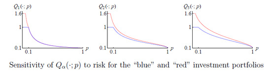
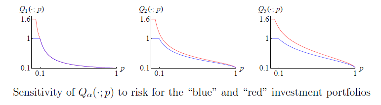
5.2. The Spectrum Parameter α as a Risk Sensitivity Index

Greater values of the spectrum parameter α correspond to greater sensitivity to risk; cf., e.g., [36]. This is manifested, first of all, by the monotonicity of $Q_{\alpha }(X;p)$ in α, as stated in Theorem 3.4). (In the normal-distribution realm, this monotonicity is expressed as the growing (with α) weight of the standard deviation σ of the loss X in its linear combination with the mean μ in (3.12).)

Moreover, in view of the monotonicity in X (also stated in Theorem 3.4) and Proposition 3.5, the sensitivity index α is in a one-to-one correspondence with the highest order of the stochastic dominance respected by $Q_{\alpha }(X;p)$.

As pointed out in the Introduction, the most popular coherent risk measure $CVaR$ has a fixed and rather limited sensitivity to risk and thus allows of no variation in the degree of such sensitivity. In fact, one can easily construct two investment portfolios such that

(i)

one of the portfolios is clearly riskier than the other;

(ii)

this distinction is sensed (to varying degrees, depending on α) by all the risk measures $Q_{\alpha }(X;p)$ with $\alpha \in (1,\infty )$;

(iii)

yet, the values of ${CVaR}_p=Q_1(X;p)$ are the same for both portfolios.

For instance, let X and Y denote the potential losses corresponding to two different investments portfolios. Suppose that there are mutually exclusive events $E_1$ and $E_2$ and real numbers $p_{*}\in (0,1)$ and $\delta \in (0,1)$ such that (i) $\mathsf{P}(E_1)=\mathsf{P}(E_2)=p_{*}/2$; (ii) the loss of either portfolio is 0 if the event $E_1\cup E_2$ does not occur; (iii) the loss of the X-portfolio is 1 if the event $E_1\cup E_2$ occurs; and (iv) the loss of the Y-portfolio is $1-\delta$ if the event $E_1$ occurs, and it is $1+\delta$ if the event $E_2$ occurs. Thus, the r.v. X takes values 0 and 1 with probabilities $1-p_{*}$ and $p_{*}$, and the r.v. Y takes values 0, $1-\delta$, and $1+\delta$ with probabilities $1-p_{*}$, $p_{*}/2$, and $p_{*}/2$, respectively. Hence, $\mathsf{E}X=\mathsf{E}Y$, that is, the expected losses of the two portfolios are the same. Clearly, the distribution of X is less dispersed than that of Y, both intuitively and also in the formal sense that $X\stackrel{\alpha +1}{⩽}Y$ for all $\alpha \in [1,\infty ]$. So, everyone will probably say that the Y-portfolio is riskier than the X-portfolio. However, for any $p\in (p_{*},1)$ it is easy to see, by (3.3), that $Q_0(X;p)=0=Q_0(Y;p)$, and hence, in view of (5.10), $Q_1(Y;p)=\frac{1}{p}\mathsf{E}Y=\frac{p_{*}}{p}=\frac{1}{p}\mathsf{E}X=Q_1(X;p)$. Using also the continuity of $Q_{\alpha }(·;p)$ in p, as stated in Theorem 3.4, one concludes that the $Q_1(·;p)={CVaR}_p(·)$ risk value of the riskier Y-portfolio is the same as that of the less risky X-portfolio for all $p\in [p_{*},1)$. Such indifference (which may also be referred to as insufficient sensitivity to risk) may generally be considered “an unwanted characteristic” – see e.g. pages 36 and 48 in [4]. One can also perceive the exhibited here lack of dependence of $CVaR$ on δ as a certain “flatness” of this measure of risk.

Let us now show that, in contrast with the risk measure $Q_1(·;p)={CVaR}_p(·)$, the value of $Q_{\alpha }(·;p)$ is sensitive to risk for all $\alpha \in (1,\infty )$ and all $p\in (0,1)$; that is, for all such α and p and for the losses X and Y as above, $Q_{\alpha }(Y;p)>Q_{\alpha }(X;p)$. Indeed, take any $\alpha \in (1,\infty )$. By (2.17) and (4.10), $x_{*,X}=1$, $p_{*,X}=p_{*}$, $x_{*,Y}=1+\delta$, $x_{**,Y}=1-\delta$, and $p_{*,Y}=p_{*}/2$. If $p\in (0,p_{*}/2]$ then, by Part (ii) of Proposition 3.1, $Q_{\alpha }(Y;p)=x_{*,Y}=1+\delta >1=x_{*,X}=Q_{\alpha }(X;p)$. If now $p\in (p_{*}/2,1)$, then, by Formula (3.20) in [8, $t_Y:={}_{\alpha -1}Q(Y;p)\in (-\infty ,x_{**,Y})=(-\infty ,1-\delta )$. Also, by a strict version of Jensen’s inequality and the strict convexity of $u^{\alpha }$ in $u\in [0,\infty )$, $B_{\alpha }(X;p)(t)=t+p^{-1/\alpha }{\parallel X-t\parallel }_{\alpha }<t+p^{-1/\alpha }{\parallel Y-t\parallel }_{\alpha }=B_{\alpha }(Y;p)(t)$ for all $t\in (-\infty ,1-\delta ]$. Therefore, by Formula (3.18) in [8] and Formula (3.8) in the present paper, $Q_{\alpha }(Y;p)=B_{\alpha }(Y;p)(t_Y)>B_{\alpha }(X;p)(t_Y)⩾Q_{\alpha }(X;p)$. Thus, it is checked that $Q_{\alpha }(Y;p)>Q_{\alpha }(X;p)$ for all $\alpha \in (1,\infty )$ and all $p\in (0,1)$.

The above example is illustrated in Figure 4, for $p_{*}=0.1$ and $\delta =0.6$. It is seen that the sensitivity of the measure $Q_{\alpha }(·;p)$ to risk (reflected especially by the gap between the red and blue lines for $p\in [p_{*},1)=[0.1,1)$) increases from the zero sensitivity when $\alpha =1$ to an everywhere positive sensitivity when $\alpha =2$ to an everywhere greater positive sensitivity when $\alpha =5$.

Figure 4. Sensitivity of $Q_{\alpha }(·;p)$ to risk, depending on the value of α: graphs $\left\{\left(p,Q_{\alpha }(X;p)\right):0<p<1\right\}$ (blue) and $\left\{\left(p,Q_{\alpha }(Y;p)\right):0<p<1\right\}$ (red) for $\alpha =1$ (left); $\alpha =2$ (middle); and $\alpha =5$ (right).

Figure 4. Sensitivity of $Q_{\alpha }(·;p)$ to risk, depending on the value of α: graphs $\left\{\left(p,Q_{\alpha }(X;p)\right):0<p<1\right\}$ (blue) and $\left\{\left(p,Q_{\alpha }(Y;p)\right):0<p<1\right\}$ (red) for $\alpha =1$ (left); $\alpha =2$ (middle); and $\alpha =5$ (right).

That ${CVaR}_p=Q_1(·;p)$ is flat – in contrast to $Q_{\alpha }(·;p)$ with $\alpha \in (1,\infty )$ – is of course rooted in the fact that $u^{\alpha }$ is strictly convex in $u\in [0,\infty )$ only for $\alpha \in (1,\infty )$, but not for $\alpha =1$; cf. e.g. [37], where it is shown that the normed space ${\mathcal{L}}^{\alpha }$ is uniformly convex for $\alpha \in (1,\infty )$ (but of course not for $\alpha =1$).

5.3. Coherent and Non-Coherent Measures of Risk

Based on an extensive and penetrating discussion of methods of measurement of market and non-market risks, Artzner et al. [1] concluded that, for a risk measure to be effective in risk regulation and management, it has to be coherent, in the sense that it possess the translation invariance, subadditivity, positive homogeneity, and monotonicity properties. In general, a risk measure, say $\widehat{\rho }$, is a mapping of a linear space of real-valued r.v.’s on a given probability space into $\mathbb{R}$. The probability space (say Ω) was assumed to be finite in [1]. More generally, one could allow Ω to be infinite, and then it is natural to allow $\widehat{\rho }$ to take values $\pm \infty$ as well. In [1], the r.v.’s (say Y) in the argument of the risk measure were called risks but at the same time interpreted as “the investor’s future net worth”. Then the translation invariance was defined in [1] as the identity $\widehat{\rho }(Y+rt)=\widehat{\rho }(Y)-t$ for all r.v.’s Y and real numbers t, where r is a positive real number, interpreted as the rate of return. We shall, however, follow Pflug [26] (among other authors), who considers a risk measure (say ρ) as a function of the potential cost/loss, say X, and then defines the translation invariance of ρ, quite conventionally, as the identity $\rho (X+c)=\rho (X)+c$ for all r.v.’s X and real numbers c. The approaches in [1,26] are equivalent to each other, and the correspondence between them can be given by the formulas $\rho (X)=r\widehat{\rho }(Y)=r\widehat{\rho }(-X)$, $X=-Y$, and $c=-rt$. The positive homogeneity, as defined in [1], can be stated as the identity $\rho (\lambda X)=\lambda \rho (X)$ for all r.v.’s X and real numbers $\lambda ⩾0$.

Corollary 5.1. For each $\alpha \in [1,\infty ]$ and each $p\in (0,1)$, the quantile bound $Q_{\alpha }(·;p)$ is a coherent risk measure, and it is not coherent for any pair $(\alpha ,p)\in [0,1)\times (0,1)$.

This follows immediately from Theorem 3.4 and Proposition 3.7.

The usually least trivial of the four properties characterizing the coherence is the subadditivity of a risk measure – which, in the presence of the positive homogeneity, is equivalent to the convexity, as was pointed out earlier in this paper. As is well known and also discussed above, the value at risk measure ${VaR}_p(X)$ is translation invariant, positive homogeneous, and monotone (in X), but it fails to be subadditive. Quoting from page 1458 in [2]: “The coherence of [${CVaR}_p(X)$] is a formidable advantage not shared by any other widely applicable measure of risk yet proposed.”

Corollary 5.1 above addresses this problem by providing an entire infinite family of coherent risk measures, indexed by $\alpha \in [1,\infty ]$, including ${CVaR}_p=Q_1(·;p)$ just as one member of the family. Moreover, ${CVaR}_p$ can now be seen as only “barely”, borderline coherent – because (${CVaR}_p=Q_1(·;p)$ and) $\alpha =1$ is the smallest value of the sensitivity index for which the risk measure $Q_{\alpha }(·;p)$ is coherent. One can also say that the coherence of $CVaR$ is unstable with respect to the sensitivity index α: ${CVaR}_p$ is coherent, but the risk measure $Q_{\alpha }(·;p)$ (which is arbitrarily close to ${CVaR}_p$ when α is close enough to 1) is not coherent if $\alpha \in [0,1)$. Here one may also recall the discussion in Section 5.2 on $CVaR$’s “flatness” and indifference to risk.

5.4. Other Terminology Used in the Literature for Some of the Listed Properties of $Q_{\alpha }(·;p)$

Theorem 3.4 provides a number of useful properties of the spectrum of risk measures $Q_{\alpha }(·;p)$. The terminology we use to name some of these properties differs from the corresponding terminology used elsewhere.

In particular, what we refer to as the “positive sensitivity” in Theorem 3.4 corresponds to the “relevance” in [1].

Next, in the present paper the “model-independence” means that the risk measure depends on the potential loss only through the distribution of the loss, rather than on the way to model the “states of nature”, on which the loss may depend. In contrast, in [1] a measure of risk is considered “model-free” if it does not depend, not only on modeling the “states of nature”, but, to a possibly large extent, on the distribution of the loss. An example of such a “model-free” risk measure is given by the SEC rules mentioned in Section 4.4; this measure of risk depends only on the set of all possible representations of the investment portfolio in question as a portfolio of long call spreads, that is, pairs of the form (a long call, a short call). If a measure of risk is not “model-free”, then it is called “model-dependent” in [1]. The “model-independence” property is called “law-invariance” in Section 12.1.2 of [38], and a similar property is called “neutrality” on page 97 in [39].

Also in [38], the consistency property is referred to as “constancy”.

5.5. Gini-Type Mean Differences and Related Risk Measures

Yitzhaki [40] utilized the Gini mean difference – which had prior to that been mainly used as a measure of economic inequality – to construct, somewhat implicitly, a measure of risk; this approach was further developed in [41,42]. If (say) a r.v. X is thought of as the income of a randomly selected person in a certain state, then the Gini mean difference can be defined by the formula

$$G_H(X):=\mathsf{E}H(|X-\tilde{X}|),$$

where $\tilde{X}$ is an independent copy of X and $H:[0,\infty )\to \mathbb{R}$ is a measurable function, usually assumed to be nonnegative and such that $H(0)=0$; clearly, given the function H, the Gini mean difference $G_H(X)$ depends only on the distribution of the r.v. X. Therefore, if $H(u)$ is considered, for any $u\in [0,\infty )$, as the measure of inequality between two individuals with incomes x and y such that $|x-y|=u$, then the Gini mean difference $\mathsf{E}H(|X-\tilde{X}|)$ is the mean H-inequality in income between two individuals selected at random (and with replacement, thus independently of each other). The most standard choice for H is the identity function $id$, so that $H(u)=id(u)=u$ for all $u\in [0,\infty )$. Based on the measure-of-inequality $G_H$, one can define the risk measure

$$R_H(X):=\mathsf{E}X+G_H(X)=\mathsf{E}X+\mathsf{E}H(|X-\tilde{X}|),$$

(5.2)

where now the r.v. X is interpreted as the uncertain loss on a given investment, with the term $G_H(X)=\mathsf{E}H(|X-\tilde{X}|)$ then possibly interpreted as a measure of the uncertainty. Clearly, when there is no uncertainty, so that the loss X is in fact a nonrandom real constant, then the measure $G_H(X)$ of the uncertainty is 0, assuming that $H(0)=0$. If $X\sim N(\mu ,{\sigma }^2)$ (that is, X is normally distributed with mean μ and standard deviation $\sigma >0$) and $H=\kappa id$ for some positive constant κ, then $R_H(X)=\mu +\frac{2\kappa }{\sqrt{\pi }}\sigma$, a linear combination of the mean and the standard deviation, so that in such a case we find ourselves in the realm of the Markowitz mean-variance risk-assessment framework; cf. (3.12).

It is assumed that $R_H(X)$ is defined when both expected values in the last expression in (5.2) are defined and are not infinite values of opposite signs – so that these two expected values could be added, as needed in (5.2).

It is clear that $R_H(X)$ is translation-invariant. Moreover, $R_H(X)$ is convex in X if the function H is convex and nondecreasing. Further, if $H=\kappa id$ for some positive constant κ, then $R_H(X)$ is also positive-homogeneous.

It was shown in [40], under an additional technical condition, that $R_H(X)$ is nondecreasing in X with respect to the stochastic dominance of order 1 if $H=\frac{1}{2}id$. Namely, the result obtained in [40] is that if $X\stackrel{\mathrm{st}}{⩽}Y$ and the distribution functions F and G of X and Y are such that $F-G$ changes sign only finitely many times on $\mathbb{R}$, then $R_{\frac{1}{2}id}(X)⩽R_{\frac{1}{2}id}(Y)$. A more general result was obtained in [42], which can be stated as follows: in the case when the function H is differentiable, $R_H(X)$ is nondecreasing in X with respect to the stochastic dominance of order one if and only if $|H^{\prime }|⩽\frac{1}{2}$. Cf. also [41]. The proof in [42] was rather long and involved; in addition, it used a previously obtained result of [43]. Here we are going to give (in Appendix A) a very short, direct, and simple proof of the more general

Proposition 5.2. The risk measure $R_H(X)$ is nondecreasing in X with respect to the stochastic dominance of order 1 if and only if the function H is $\frac{1}{2}$-Lipschitz: $|H(x)-H(y)|⩽\frac{1}{2}|x-y|$ for all x and y in $[0,\infty )$.

In Proposition 5.2, it is not assumed that $H⩾0$ or that $H(0)=0$. Of course, if H is differentiable, then the $\frac{1}{2}$-Lipschitz condition is equivalent to the condition $|H^{\prime }|⩽\frac{1}{2}$ in [42].

The risk measure $R_H(X)$ was called mean-risk (M-R) in [41].

It follows from [42] or Proposition 5.2 above that the risk measure $R_{\kappa id}(X)$ is coherent for any $\kappa \in [0,\frac{1}{2}]$. In fact, based on Proposition 5.2, one can rather easily show more:

Proposition 5.3. The risk measure $R_H(X)$ is coherent if and only if $H=\kappa id$ for some $\kappa \in [0,\frac{1}{2}]$.

It is possible to indicate a relation – albeit rather indirect – of the risk measure $R_H(X)$, defined in (5.2), with the quantile bounds $Q_{\alpha }(X;p)$. Indeed, introduce

$${\widehat{Q}}_{\alpha }(X;p)=\mathsf{E}X+p^{-1/\alpha }\parallel {(X-\mathsf{E}X)}_{+}{\parallel }_{\alpha },$$

(5.3)

assuming $\mathsf{E}X$ exists in $\mathbb{R}$. By (3.8)–(3.9), ${\widehat{Q}}_{\alpha }(X;p)$ is a majorant of $Q_{\alpha }(X;p)$, obtained by using $t=\mathsf{E}X$ in (3.8) as a surrogate of the minimizing value of t.

The term $p^{-1/\alpha }\parallel {(X-\mathsf{E}X)}_{+}{\parallel }_{\alpha }$ in (5.3) is somewhat similar to the Gini mean-difference term $\mathsf{E}H(|X-\tilde{X}|)$, at least when $\alpha =1$ and (the distribution of) the r.v. X is symmetric about its mean.

Moreover, if the distribution of $X-\mathsf{E}X$ is symmetric and stable with index $\gamma \in (1,2]$, then ${\widehat{Q}}_1(X;p)=R_{\kappa id}(X)$ with $\kappa =2^{-1-1/\gamma }/p$.

One may want to compare the two considered kinds of coherent measures of risk/inequality, $R_{\kappa id}(X)$ for $\kappa \in [0,\frac{1}{2}]$ and $Q_{\alpha }(X;p)$ for $\alpha \in [1,\infty ]$ and $p\in (0,1)$. It appears that the latter measure is more flexible, as it depends on two parameters (α and p) rather than just one parameter (κ). Moreover, as previously mentioned Proposition 2.7 in [8] shows, rather generally $Q_{\alpha }(X;p)$ retains a more or less close relation with the quantile $Q_0(X;p)$ – which, recall, is the widely used value at risk (VaR). On the other hand, recall here that, in contrast with the VaR, $Q_{\alpha }(X;p)$ is coherent for $\alpha \in [1,\infty ]$. However, both of these kinds of coherent measures appear useful, each in its own manner, representing two different ways to express risk/inequality.

Formulas (5.2) and (5.3) can be considered special instances of the general relation between risk measures and measures of inequality established in [44]. Let ${\mathcal{X}}_{\mathsf{E}}$ be a convex cone of real-valued r.v. $X\in \mathcal{X}$ with a finite mean $\mathsf{E}X$ such that ${\mathcal{X}}_{\mathsf{E}}$ contains all real constants.

Largely following [44] (see also the earlier study [45]), let us say a coherent risk measure $R:{\mathcal{X}}_{\mathsf{E}}\to (-\infty ,\infty ]$ is strictly expectation-bounded if $R(X)>\mathsf{E}X$ for all $X\in {\mathcal{X}}_{\mathsf{E}}$. (Note that here the r.v. X represents the loss, whereas in [44] it represents the gain; accordingly, X in this paper corresponds to $-X$ in [44]; also, in [44] the cone ${\mathcal{X}}_{\mathsf{E}}$ was taken to be the space ${\mathcal{L}}^2$.) In view of Theorem 3.4 and Part (vii) of Proposition 3.1, it follows that $Q_{\alpha }(X;p)$ is a coherent and strictly expectation-bounded risk measure if $\alpha \in [1,\infty ]$. Also (cf. Definition 1 and Proposition 1 in [44]), let us say that a mapping $D:{\mathcal{X}}_{\mathsf{E}}\to [0,\infty ]$ is a deviation measure if D is subadditive, positive-homogeneous, and nonnegative with $D(X)=0$ if and only if $\mathsf{E}(X=c)=1$ for some real constant c; here X is any r.v. in ${\mathcal{X}}_{\mathsf{E}}$. Next (cf. Definition 2 in [44]), let us say that a deviation measure $D:{\mathcal{X}}_{\mathsf{E}}\to [0,\infty ]$ is upper-range dominated if $D(X)⩽supsuppX-\mathsf{E}X$ for all $X\in {\mathcal{X}}_{\mathsf{E}}$. Then (cf. Theorem 2 in [44]), the formulas

$$D(X)=R(X-\mathsf{E}X)\text{and}R(X)=\mathsf{E}X+D(X)$$

(5.4)

provide a one-to-one correspondence between all coherent strictly expectation-bounded risk measures $R:{\mathcal{X}}_{\mathsf{E}}\to (-\infty ,\infty ]$ and all upper-range dominated deviation measures $D:{\mathcal{X}}_{\mathsf{E}}\to [0,\infty ]$.

In particular, it follows that the risk measure ${\widehat{Q}}_{\alpha }(·;p)$, defined by Formula (5.3), is coherent for all $\alpha \in [1,\infty ]$ and all $p\in (0,\infty )$. It also follows that $X\mapsto Q_{\alpha }(X-\mathsf{E}X;p)$ is a deviation measure. As was noted, ${\widehat{Q}}_{\alpha }(X;p)$ is a majorant of $Q_{\alpha }(X;p)$. In contrast with $Q_{\alpha }(X;p)$, in general ${\widehat{Q}}_{\alpha }(X;p)$ will not have such a close hereditary relation with the true quantile $Q_0(X;p)$ as e.g. the ones given in the previously mentioned Proposition 2.7 in [8]. For instance, if $\mathsf{P}(X⩾x)$ is like $x^{-\infty }$ then, by Formulas (2.13)-(2.14) in [8, $Q_{\alpha }(X;p)\underset{p\downarrow 0}{\sim }{Q}_0(X;p)$ for each $\alpha \in [0,\infty ]$, whereas ${\widehat{Q}}_{\infty }(X;p)=\infty$ for all real $p>0$. On the other hand, in distinction with the definition (5.3) of ${\widehat{Q}}_{\alpha }(X;p)$, the expression (3.8) for $Q_{\alpha }(X;p)$ requires minimization in t; however, that minimization will add comparatively little to the complexity of the problem of minimizing $Q_{\alpha }(X;p)$ subject to a usually large number of restrictions on X; cf. Theorem 4.7. Risk measures similar to (5.3) were considered in [46] in relation with the stochastic dominance of arbitrary orders.

5.6. A Lorentz-Type Parametric Family of Risk Measures

Recalling (2.29) and following [21,22,47], one may also consider $-F_{-X}^{(-\alpha )}(p)$ as a measure of risk. Here one will need the following semigroup identity, given by Formula (8a) in [21], (cf. e.g. Remark 3.7 in [5]):

$$F_X^{(-\alpha )}(p)=\frac{1}{\Gamma (\alpha -\nu )}{\int }_0^p{(p-u)}^{\alpha -\nu -1}{F}_X^{(-\nu )}(u)\text{d}u$$

(5.5)

whenever $0<\nu <\alpha <\infty$. The following proposition is well known.

Proposition 5.4. If the r.v. X is nonnegative, then

$$F_X^{(-2)}(p)=L_X(p)=-p{CVaR}_p(-X),$$

(5.6)

where $L_X$ is the Lorenz curve function, given by the formula

$$L_X(p):={\int }_0^p{F}_X^{-1}(u)\text{d}u$$

(5.7)

.

Indeed, the first equality in (5.6) is the special case of the identity (5.5) with $\alpha =2$ and $\nu =1$, and the second equality in (5.6) follows by Part (i) of Theorem 3.1 in [48], identity (3.8) for $\alpha =1$, and the second identity in (5.1). Cf. Theorem 2 in [49] and [20,50].

Using (5.5) with $\nu =2$, $\alpha +1$ in place of α, and $-X$ in place of X together with Proposition 5.4, one has

$$-F_{-X}^{(-\alpha -1)}(p)=\frac{1}{\Gamma (\alpha -1)}{\int }_0^p{(p-u)}^{\alpha -2}u{CVaR}_u(X)\text{d}u$$

(5.8)

for any $\alpha \in (1,\infty )$. Since ${CVaR}_u(X)$ is a coherent risk measure, it now follows that, as noted in [47], $-F_{-X}^{(-\alpha -1)}(p)$ is a coherent risk measure as well, again for $\alpha \in (1,\infty )$; by (5.6), this conclusion will hold for $\alpha =1$. However, one should remember that the expression $F_X^{(-\alpha )}(p)$ was defined only when the r.v. X is nonnegative (and otherwise some of the crucial considerations above will not hold). Thus, $-F_{-X}^{(-\alpha -1)}(p)$ is defined only if $X⩽0$ almost surely.

5.7. Spectral Risk Measures

In view of (5.8), the risk measure $-F_{-X}^{(-\alpha -1)}(p)$ is a mixture of the coherent risk measures ${CVaR}_u(X)$ and thus a member of the general class of the so-called spectral risk measures [51], which are precisely the mixtures, over the values $u\in (0,1)$, of the risk measures ${CVaR}_u(X)$; thus, all spectral risk measures are automatically coherent. However, in general such measures will lack such an important variational representation as the one given by Formula (3.8) for the risk measure $Q_{\alpha }(X;p)$. Of course, for any “mixing” nonnegative Borel measure μ on the interval $(0,1)$ and the corresponding spectral risk measure ${CVaR}_{\mu }(X):={\int }_{(0,1)}{CVaR}_u(X)\mu (\text{d}u)$, one can write

$${CVaR}_{\mu }(X)={\int }_{(0,1)}\underset{t\in \mathbb{R}}{inf}\left(t+\frac{1}{u}{\parallel {(X-t)}_{+}\parallel }_1\right)\mu (\text{d}u),$$

(5.9)

in view of (5.1) and (3.8)–(3.9). However, in contrast with (3.8), the minimization (in $t\in \mathbb{R}$) in (5.9) needs in general to be done for each of the infinitely many values of $u\in (0,1)$. If the r.v. X takes only finitely many values, then the expression of ${CVaR}_{\mu }(X)$ in (5.9) can be rewritten as a finite sum, so that the minimization in $t\in \mathbb{R}$ will be needed only for finitely many values of u; cf. e.g. the optimization problem on page 8 in [47].

On the other hand, one can of course consider arbitrary mixtures in $p\in (0,1)$ and/or $\alpha \in [1,\infty )$ of the risk measures $Q_{\alpha }(X;p)$. Such mixtures will automatically be coherent. Also, all mixtures of the measures $Q_{\alpha }(X;p)$ in p will be nondecreasing in α, and all mixtures of $Q_{\alpha }(X;p)$ in α will be nonincreasing in p.

5.8. Risk Measures Reinterpreted as Measures of Economic Inequality

Deviation measures such as the ones studied in [44] and discussed in the paragraph containing (5.4) can be used as measures of economic inequality if the r.v. X models, say, the random income/wealth – defined as the income/wealth of an (economic) unit chosen at random from a population of such units. Then, according to the one-to-one correspondence given by (5.4), coherent risk measures R translate into deviation measures D, and vice versa.

However, the risk measures $Q_{\alpha }(·;p)$ themselves can be used to express certain aspects of economic inequality directly, without translation into deviation measures. For instance, if X stands for the random wealth, then the statement $Q_1(X;0.01)=30\mathsf{E}X$ formalizes the common kind of expression “the wealthiest 1% own 30% of all wealth”, provided that the wealthiest 1% can be adequately defined, say as follows: there is a threshold wealth value t such that the number of units with wealth greater than or equal to t is $0.01N$, where N is the number of units in the entire population. Then (cf. (5.12)), $0.01N{Q}_1(X;0.01)=0.01N\mathsf{E}(X|X⩾t)=N\mathsf{E}X\mathsf{I}\{X⩾t\}=0.30N\mathsf{E}X$, whence indeed $Q_1(X;0.01)=30\mathsf{E}X$. Similar in spirit expressions of economic inequality in terms of $Q_{\alpha }(X;p)$ can be provided for all $\alpha \in (0,\infty )$. For instance, suppose now that X stands for the annual income of a randomly selected household, whereas x is a particular annual household income level in question. Then, in view of (3.8)–(3.9), the inequality $Q_{\alpha }(X;p)⩾x$ means that for any (potential) annual household income level t less than the maximum annual household income level $x_{*,X}$ in the population, the conditional α-mean $\mathsf{E}{\left({(X-t)}^{\alpha }|X>t\right)}^{1/\alpha }$ of the excess ${(X-t)}_{+}$ of the random income X over t is no less than ${\left(\frac{p}{\mathsf{E}(X>t)}\right)}^{1/\alpha }$ times the excess ${(x-t)}_{+}$ of the income level x over t. Of course, the conditional α-mean $\mathsf{E}{\left({(X-t)}^{\alpha }|X>t\right)}^{1/\alpha }$ is increasing in α. Thus, using the measure $Q_{\alpha }(X;p)$ of economic inequality with a greater value of α means treating high values of the economic variable X in a more progressive/sensitive manner. One may also note here that the above interpretation of the inequality $Q_{\alpha }(X;p)⩾x$ is a “synthetic” statement in the sense that it provides information concerning all values of potential interest of the threshold annual household income level t.

Not only the upper bounds $Q_{\alpha }(X;p)$ on the quantile $Q(X;p)$, but also the upper bounds ${\mathsf{P}}_{\alpha }(X;x)$ on the tail probability $\mathsf{P}(X⩾x)$ may be considered measures of risk/inequality. Indeed, if X is interpreted as the potential loss, then the tail probability $\mathsf{P}(X⩾x)$ corresponds to the classical safety-first (SF) risk measure; see e.g. [52,53].

5.9. “Explicit” Expressions of $Q_{\alpha }(X;p)$

In the case $\alpha =1$, an expression of $Q_{\alpha }(X;p)$ can be given in terms of the true $(1-p)$-quantile $Q(X;p)$:

$$Q_1(X;p)=Q(X;p)+\frac{1}{p}\mathsf{E}{\left(X-Q(X;p)\right)}_{+}.$$

(5.10)

That the expression for $Q_1(X;p)$ in (3.8) coincides with the one in (5.10) was established in Theorem 1 in [3] for absolutely continuous r.v.’s X, and then on page 273 in [26] and in Theorem 10 in [2] in general. For the readers’ convenience, let us present here the following brief proof of (5.10). For all real $h>0$ and $t\in \mathbb{R}$, one has

$${(X-t)}_{+}-{(X-t-h)}_{+}=h\mathsf{I}\{X>t\}-(t+h-X)\mathsf{I}\{t<X<t+h\}.$$

It follows that the right derivative of the convex function ${t\mapsto t+\parallel (X-t)}_{+}{\parallel }_1/p$ at any point $t\in \mathbb{R}$ is $1-\mathsf{P}(X>t)/p$, which, by (3.3), is $⩽0$ if $t<Q(X;p)$ and $>0$ if $t>Q(X;p)$. Hence, $Q(X;p)$ is a minimizer in $t\in \mathbb{R}$ of ${t+\parallel (X-t)}_{+}{\parallel }_1/p$, and thus (5.10) follows by (3.8). It is also seen now that any $(1-p)$-quantile of X is a minimizer in $t\in \mathbb{R}$ of ${t+\parallel (X-t)}_{+}{\parallel }_1/p$ as well, and $Q(X;p)$ is the largest of these minimizers.

As was shown in [2], the expression for $Q_1(X;p)$ in (5.10) can be rewritten as a conditional expectation:

$$\begin{array}{cc}\hfill Q_1(X;p)& =Q(X;p)+\mathsf{E}\left(X-Q(X;p)|X⩾Q(X;p),U⩾\delta \right)\hfill \\ & =\mathsf{E}\left(X|X⩾Q(X;p),U⩾\delta \right),\hfill \end{array}$$

(5.11)

where U is any r.v. which is independent of X and uniformly distributed on the interval $[0,1]$, $\delta :=\delta (X;p):=d\mathsf{I}\{X=Q(X;p)\}$, and d is any real number in the interval $[0,1]$ such that

$$\mathsf{P}\left(X⩾Q(X;p)\right)-p=\mathsf{P}\left(X=Q(X;p)\right)d;$$

such a number d always exists. Thus, the r.v. U is used to split the possible atom of the distribution of X at the quantile point $Q(X;p)$ in order to make the randomized tail probability $\mathsf{P}\left(X⩾Q(X;p),U⩾\delta \right)$ exactly equal to p. Of course, in the absence of such an atom, one can simply write

$$Q_1(X;p)=Q(X;p)+\mathsf{E}\left(X-Q(X;p)|X⩾Q(X;p)\right)=\mathsf{E}\left(X|X⩾Q(X;p)\right).$$

(5.12)

As pointed out in [2,3] and discussed in Section 4.3, a variational formula such as (3.8) has a distinct advantage over such ostensibly explicit formulas as (5.10) and (5.11), since (3.8) allows of rather easy incorporation into specialized optimization problems. Nonetheless, one can obtain an extension of the representation (5.10), valid for all $\alpha \in [1,\infty )$; see Formula (4.18) and also Proposition 4.7 in [8].

6. Conclusions

Let us summarize some of the advantages of the risk/inequality measures $P_{\alpha }(X;x)$ and $Q_{\alpha }(X;p)$:

• $P_{\alpha }(X;x)$ and $Q_{\alpha }(X;p)$ are three-way monotonic and three-way stable – in α, p, and X.
• The monotonicity in X is graded continuously in α, resulting in varying, controllable degrees of sensitivity of $P_{\alpha }(X;x)$ and $Q_{\alpha }(X;p)$ to financial risk/economic inequality.
• $x\mapsto P_{\alpha }(X;x)$ is the tail-function of a certain probability distribution.
• $Q_{\alpha }(X;p)$ is a $(1-p)$-percentile of that probability distribution.
• For small enough values of p, the quantile bounds $Q_{\alpha }(X;p)$ are close enough to the corresponding true quantiles $Q(X;p)={VaR}_p(X)$, provided that the right tail of the distribution of X is light enough and regular enough, depending on α.
• In the case when the loss X is modeled as a normal r.v., the use of the risk measures $Q_{\alpha }(X;p)$ reduces, to an extent, to using the Markowitz mean-variance risk-assessment paradigm – but with a varying weight of the standard deviation, depending on the risk sensitivity parameter α.
• $P_{\alpha }(X;x)$ and $Q_{\alpha }(X;p)$ are solutions to mutually dual optimizations problems, which can be comparatively easily incorporated into more specialized optimization problems, with additional restrictions on the r.v. X.
• $P_{\alpha }(X;x)$ and $Q_{\alpha }(X;p)$ are effectively computable.
• Even when the corresponding minimizer is not identified quite perfectly, one still obtains an upper bound on the risk/inequality measures $P_{\alpha }(X;x)$ or $Q_{\alpha }(X;p)$.
• Optimal upper bounds on $P_{\alpha }(X;x)$ and, hence, on $Q_{\alpha }(X;p)$ over important classes of r.v.’s X represented (say) as sums of independent r.v.’s $X_i$ with restrictions on moments of the $X_i$’s and/or sums of such moments can be given; see e.g. [7,54] and references therein.
• The quantile bounds $Q_{\alpha }(X;p)$ with $\alpha \in [1,\infty ]$ constitute a spectrum of coherent measures of financial risk and economic inequality.
• The r.v.’s X of which the measures $P_{\alpha }(X;x)$ and $Q_{\alpha }(X;p)$ are taken are allowed to take values of both signs. In particular, if, in a context of economic inequality, X is interpreted as the net amount of assets belonging to a randomly chosen economic unit, then a negative value of X corresponds to a unit with more liabilities than paid-for assets. Similarly, if X denotes the loss on a financial investment, then a negative value of X will obtain when there actually is a net gain.

As seen from the discussion in Section 5, some of these advantages, and especially their totality, appear to be unique to the risk measures proposed here.

Further studies involving especially the use and computational implementation of the proposed risk measures would be welcome.

References

1. P. Artzner, F. Delbaen, J.-M. Eber, and D. Heath. “Coherent measures of risk.” Math. Financ. 9 (1999): 203–228. [Google Scholar] [CrossRef]
2. R.T. Rockafellar, and S. Uryasev. “Conditional value at risk for general loss distributions.” J. Bank. Financ. 26 (2002): 1443–1471. [Google Scholar] [CrossRef]
3. R.T. Rockafellar, and S. Uryasev. “Optimization of conditional value at risk.” J. Risk 2 (2000): 21–41. [Google Scholar]
4. H. Grootveld, and W.G. Hallerbach. Upgrading value at risk from diagnostic metric to decision variable: A wise thing to do? In Risk Measures in the 21st Century. Hoboken, NJ, USA: Wiley, 2004, pp. 33–50. [Google Scholar]
5. I. Pinelis. “Optimal tail comparison based on comparison of moments.” In High Dimensional Probability (Oberwolfach, 1996). Basel, Switzerland: Birkhäuser, 1998, Volume 43, pp. 297–314. [Google Scholar]
6. I. Pinelis. “On the Bennett-Hoeffding Inequality.” 2009. Available online: http://arxiv.org/abs/0902.4058 (accessed on 24 February 2009).
7. I. Pinelis. “On the Bennett–Hoeffding inequality.” Annales de l’Institut Henri Poincaré, Probabilités et Statistiques 50 (2014): 15–27. [Google Scholar] [CrossRef]
8. I. Pinelis. “An Optimal Three-Way Stable and Monotonic Spectrum of Bounds On Quantiles: A Spectrum of Coherent Measures of Financial Risk and Economic Inequality, Version 1.” 2013. Available online: http://arxiv.org/abs/1310.6025 (accessed on 24 October 2013).
9. I. Pinelis. “Fractional sums and integrals of r-concave tails and applications to comparison probability inequalities.” In Advances in Stochastic Inequalities (Atlanta, GA, 1997). Providence, RI, USA: American Mathematical Society, 1999, Volume 234, pp. 149–168. [Google Scholar]
10. I. Pinelis. “Binomial upper bounds on generalized moments and tail probabilities of (super)martingales with differences bounded from above.” In High Dimensional Probability. Beachwood, OH, USA: Institute of Mathematical Statistics, 2006, Volume 51, pp. 33–52. [Google Scholar]
11. M.L. Eaton. “A probability inequality for linear combinations of bounded random variables.” Ann. Statist. 2 (1974): 609–613. [Google Scholar] [CrossRef]
12. J.-M. Dufour, and M. Hallin. “Improved Eaton bounds for linear combinations of bounded random variables, with statistical applications.” J. Am. Stat. Assoc. 88 (1993): 1026–1033. [Google Scholar] [CrossRef]
13. I. Pinelis. “Extremal probabilistic problems and Hotelling’s T2 test under symmetry condition.” 1991. Available online: http://arxiv.org/abs/math/0701806 (accessed on 31 January 2007).
14. I. Pinelis. “Extremal probabilistic problems and Hotelling’s T2 test under a symmetry condition.” Ann. Stat. 22 (1994): 357–368. [Google Scholar] [CrossRef]
15. P. Billingsley. Convergence of Probability Measures. New York, NY, USA: John Wiley & Sons Inc., 1968. [Google Scholar]
16. M. Shaked, and J.G. Shanthikumar. Stochastic Orders. New York, NY, USA: Springer Series in Statistics; Springer, 2007. [Google Scholar]
17. P.C. Fishburn. “Continua of stochastic dominance relations for unbounded probability distributions.” J. Math. Econ. 7 (1980): 271–285. [Google Scholar] [CrossRef]
18. P.C. Fishburn. “Continua of stochastic dominance relations for bounded probability distributions.” J. Math. Econ. 3 (1976): 295–311. [Google Scholar] [CrossRef]
19. A.B. Atkinson. “More on the measurement of inequality.” J. Econ. Inequal. 6 (2008): 277–283. [Google Scholar] [CrossRef]
20. P. Muliere, and M. Scarsini. “A note on stochastic dominance and inequality measures.” J. Econ. Theory 49 (1989): 314–323. [Google Scholar] [CrossRef]
21. S. Ortobelli, S.T. Rachev, H. Shalit, and F.J. Fabozzi. “The Theory of Orderings and Risk Probability Functionals.” 2006. Available online: http://www.google.com/url?sa=t&rct=j&q=&esrc=s&source=web&cd=1&cad=rja&ved=0CDIQFjAA&url=http (accessed on 15 July 2013).
22. S. Ortobelli, S.T. Rachev, H. Shalit, and F.J. Fabozzi. “Orderings and probability functionals consistent with preferences.” Appl. Math. Financ. 16 (2009): 81–102. [Google Scholar] [CrossRef]
23. I. Pinelis. “(Quasi)additivity Properties of the Legendre–Fenchel Transform and Its Inverse, with Applications in Probability.” 2013. Available online: http://arxiv.org/abs/1305.1860 (accessed on 5 June 2013).
24. E. Rio. Personal Communication, 2013.
25. E. De Giorgi. “Reward-risk portfolio selection and stochastic dominance.” J. Bank. Financ. 29 (2005): 895–926. [Google Scholar] [CrossRef]
26. G.C. Pflug. “Some remarks on the value at risk and the conditional value at risk.” In Probabilistic Constrained Optimization. Dordrecht, The Netherlands: Kluwer Academic Publishers, 2000, Volume 49, pp. 272–281. [Google Scholar]
27. R.M. Corless, G.H. Gonnet, D.E.G. Hare, D.J. Jeffrey, and D.E. Knuth. “On the Lambert W function.” Adv. Comput. Math. 5 (1996): 329–359. [Google Scholar] [CrossRef]
28. I. Pinelis. “Positive-part moments via the Fourier–Laplace transform.” J. Theor. Probab. 24 (2011): 409–421. [Google Scholar] [CrossRef]
29. A. Kibzun, and A. Chernobrovov. “Equivalence of the problems with quantile and integral quantile criteria.” Autom. Remote Control 74 (2013): 225–239. [Google Scholar] [CrossRef]
30. C. Acerbi, and D. Tasche. “Expected shortfall: A natural coherent alternative to value at risk.” Econ. Notes 31 (2002): 379–388. [Google Scholar] [CrossRef]
31. S.T. Rachev, S. Stoyanov, and F.J. Fabozzi. Advanced Stochastic Models, Risk Assessment, and Portfolio Optimization: The Ideal Risk, Uncertainty, and Performance Measures. Hoboken, NJ, USA: John Wiley, 2007. [Google Scholar]
32. R.H. Litzenberger, and D.M. Modest. “Crisis and non-crisis risk in financial markets: A unified approach to risk management.” In The Known, the Unknown, and Unknowable in Financial Risk Management. Princeton, NJ, USA: Princeton University Press, 2008, pp. 74–102. [Google Scholar]
33. H. Mausser, and D. Rosen. “Efficient risk/return frontiers for credit risk.” Algo Res. Q. 2 (1999): 35–47. [Google Scholar]
34. F. Bassi, P. Embrechts, and M. Kafetzaki. “Risk management and quantile estimation.” In A Practical Guide to Heavy Tails (Santa Barbara, CA, 1995). Boston, MA, USA: Birkhäuser Boston, 1998, pp. 111–130. [Google Scholar]
35. P. Embrechts, C. Klüppelberg, and T. Mikosch. Modelling Extremal Events for Insurance and Finance. New York, NY, USA: Springer, 1997. [Google Scholar]
36. P.C. Fishburn. “Mean-risk analysis with risk associated with below-target returns.” Am. Econ. Rev. 67 (1977): 116–126. [Google Scholar]
37. J.A. Clarkson. “Uniformly convex spaces.” Trans. Amer. Math. Soc. 40 (1936): 396–414. [Google Scholar] [CrossRef]
38. M. Frittelli, and E.R. Gianin. “Dynamic convex risk measures.” In Risk Measures in the 21st Century. Hoboken, NJ, USA: Wiley, 2004, pp. 227–248. [Google Scholar]
39. M.E. Yaari. “The dual theory of choice under risk.” Econometrica 55 (1987): 95–115. [Google Scholar] [CrossRef]
40. S. Yitzhaki. “Stochastic dominance, mean variance, and Gini’s mean difference.” Am. Econ. Rev. 72 (1982): 178–185. [Google Scholar]
41. A. Cillo, and P. Delquie. “Mean-risk analysis with enhanced behavioral content.” Eur. J. Oper. Res. 239 (2014): 764–775. [Google Scholar] [CrossRef]
42. P. Delquie, and A. Cillo. “Disappointment without prior expectation: A unifying perspective on decision under risk.” J. Risk Uncertain. 33 (2006): 197–215. [Google Scholar] [CrossRef]
43. M.J. Machina. “Expected utility analysis without the independence axiom.” Econometrica 50 (1982): 277–323. [Google Scholar] [CrossRef]
44. R.T. Rockafellar, S. Uryasev, and M. Zabarankin. “Generalized deviations in risk analysis.” Financ. Stoch. 10 (2006): 51–74. [Google Scholar] [CrossRef]
45. R. Mansini, W. Ogryczak, and M.G. Speranza. “LP solvable models for portfolio optimization: A classification and computational comparison.” IMA J. Manag. Math. 14 (2003): 187–220. [Google Scholar] [CrossRef]
46. W. Ogryczak, and A. Ruszczyński. “On consistency of stochastic dominance and mean-semideviation models.” Math. Program. 89 (2001): 217–232. [Google Scholar] [CrossRef]
47. S. Ortobelli, S.T. Rachev, H. Shalit, and F.J. Fabozzi. “Risk Probability Functionals and Probability Metrics Applied To Portfolio Theory.” 2007. Available online: http://www.pstat.ucsb.edu/research/papers/2006mid/view.pdf (accessed on 15 July 2013).
48. W. Ogryczak, and A. Ruszczyński. “Dual stochastic dominance and related mean-risk models.” SIAM J. Optim. 13 (2002): 60–78. [Google Scholar] [CrossRef]
49. A. Kibzun, and E.A. Kuznetsov. “Comparison of VaR and CVaR criteria.” Autom.Remote Control 64 (2003): 1154–1164. [Google Scholar] [CrossRef]
50. A.B. Atkinson. “On the measurement of inequality.” J. Econom. Theory 2 (1970): 244–263. [Google Scholar] [CrossRef]
51. C. Acerbi. “Spectral measures of risk: A coherent representation of subjective risk aversion.” J. Bank. Financ. 26 (2002): 1505–1518. [Google Scholar] [CrossRef]
52. R. Giacometti, and S. Ortobelli. “Risk measures for asset allocation models.” In Risk Measures in the 21st Century. Hoboken, NJ, USA: Wiley, 2004, pp. 69–86. [Google Scholar]
53. A.D. Roy. “Safety first and the holding of assets.” Econometrica 20 (1952): 431–449. [Google Scholar] [CrossRef]
54. I. Pinelis. “Exact inequalities for sums of asymmetric random variables, with applications.” Probab. Theory Relat. Fields 139 (2007): 605–635. [Google Scholar] [CrossRef]
55. I. Pinelis. “A Necessary and Sufficient Condition on the Stability of the Infimum of Convex Functions.” 2013. Available online: http://arxiv.org/abs/1307.3806 (accessed on 7 August 2013).
56. R.T. Rockafellar. Convex Analysis. Princeton Landmarks in Mathematics; Princeton, NJ, USA: Princeton University Press, 1997, Reprint of the 1970 original, Princeton Paperbacks. [Google Scholar]
57. E. Rio. “English translation of the monograph Théorie asymptotique des processus aléatoires faiblement dépendants (2000) by E. Rio.” 2012, Work in Progress. [Google Scholar]
58. E. Rio. “Local invariance principles and their application to density estimation.” Probab. Theory Relat. Fields 98 (1994): 21–45. [Google Scholar] [CrossRef]