
Understanding Reporting Delay in General Insurance

1
Cass Business School, City University London, 106 Bunhill Row, London EC1Y 8T2, UK
2
ETH Zurich, RiskLab, Department of Mathematics, Zurich 8092, Switzerland
3
Swiss Finance Institute, Walchestrasse 9, Zurich CH-8006, Switzerland
*
Author to whom correspondence should be addressed.
†
These authors contributed equally to this work.
Risks 2016, 4(3), 25; https://doi.org/10.3390/risks4030025
Submission received: 9 February 2016
/
Revised: 10 June 2016
/
Accepted: 29 June 2016
/
Published: 8 July 2016
(This article belongs to the Special Issue Non-Life Insurance Mathematics beyond Risk Theory: Pricing and Claims Reserving)
Abstract
:The aim of this paper is to understand and to model claims arrival and reporting delay in general insurance. We calibrate two real individual claims data sets to the statistical model of Jewell and Norberg. One data set considers property insurance and the other one casualty insurance. For our analysis we slightly relax the model assumptions of Jewell allowing for non-stationarity so that the model is able to cope with trends and with seasonal patterns. The performance of our individual claims data prediction is compared to the prediction based on aggregate data using the Poisson chain-ladder method.

1. Introduction
The aim of this paper is to understand the reporting delay function of general insurance claims. The reporting delay function is an important building block in claims reserving. We study this reporting delay function in continuous time based on real individual claims data. The data is used to calibrate a non-stationary version of the statistical model considered in Jewell [1,2]. This calibration then provides an estimation of the number of incurred but not yet reported (IBNYR) claims. The second building block in claims reserving is the modeling of the cost process of insurance claims. Jewell [1] stated in 1989: “Currently, the development of a good model for cost evolution over continuous time appears to require a long-term research effort, one that we believe will use the basic understanding of the event generation and reporting processes developed here, but will require much additional empirical effort to develop an understanding of cost-generating mechanisms and their evolution over time.” Meanwhile, there have been some improvements into this direction, see Bühlmann et al. [3], Arjas [4], Norberg [5,6], Haastrup-Arjas [7], Taylor [8,9], Herbst [10], Larsen [11], Taylor et al. [12], Jessen et al. [13], Rosenlund [14], Pigeon et al. [15], Agbeko et al. [16], Antonio-Plat [17] and Badescu et al. [18,19]. But we believe that state-of-the-art modeling is still far from having a good statistical model that can be used in daily industry practice. This may partly be explained by the fact that it is rather difficult to get access to real individual claims data.
In this paper we study individual claims data of two different portfolios: a property insurance portfolio and a casualty insurance portfolio. We choose explicit distributional models for the individual claims arrival process modeling and we calibrate these models dynamically to the data. The calibration is back-tested against the observations and compared to the (Poisson) chain-ladder method (which is applied to aggregated data). The main conclusion is that the chain-ladder method has a good performance as long as the claims process is stationary, but in non-stationary environments our individual claims estimation approach clearly outperforms the chain-ladder method.
In the next two sections we introduce the underlying statistical model and we describe the available claims data. In Section 4 we model seasonality of the claims arrival process. In Section 5 we calibrate the reporting delay function and underpin this by statistical analysis. Finally, in Section 6 we compare the individual claims modeling estimate to the classical chain-ladder method on aggregated data and we back-test the results of these two approaches. The figures and the proofs are deferred to the appendix.
2. Individual Claims Arrival Modeling
We extend the model considered in Jewell [1,2] to an inhomogeneous marked Poisson point process. We define to be the instantaneous claims frequency and to be the instantaneous exposure at time . The total exposure on time interval is given by
We consider the run-off situation after time meaning that the exposure expires at time , i.e., for . This implies that the total exposure is assumed to be finite .
Assume that the claims of the total exposure on occur at times (called accident dates or claims occurrence dates) and the claims counting process is given by
and the total number of claims is given by
Model Assumptions 1.
We assume that the claims counting process is an inhomogeneous Poisson point process with intensity .
The second ingredient that we consider is the reporting date. Assume that a given claim ℓ occurs at time then we denote its reporting date at the insurance company by . For accident date and corresponding reporting date of claim ℓ we define the reporting delay by
This motivates the study of the following inhomogeneous marked Poisson point process.
Model Assumptions 2.
We assume that describes an inhomogeneous marked Poisson process with accident dates generated by an inhomogeneous Poisson point process having intensity and with mutually independent reporting delays (marks) having a time-dependent distribution for and being independent of .
From Jewell [1,2] and Norberg [5,6] we immediately obtain the following likelihood function for parameters Λ and Θ
where denotes the density of (for parameter Θ). Observe that we use a slight abuse of notation here. In Norberg [5,6] there is an additional factor because strictly speaking Model Assumptions 2 consider ordered claims arrivals for all , whereas in Jewell [1] and in Equation (2) claims arrivals are not necessarily ordered. The aim is to calibrate this model to individual claims data, that is, we would like to calibrate claims frequency Λ and reporting delay distribution . One difficulty in this calibration lies in the fact that we have missing data, because information about occurred claims with reporting dates is not available at time . Therefore, we only observe a thinned inhomogeneous Poisson process, we also refer to Norberg [5,6].
We choose . This implies that all claims have occurred at time τ, providing . By we denoted the number of claims that are reported at time τ. The intractable likelihood (2) is then converted to, for details we refer to Jewell [1],
where we only consider reported claims ℓ with and denotes the probability that an incurred claim is reported by time . This is given by
3. Description of the Data
For the statistical analysis we consider two different European insurance portfolios: (1) line of business (LoB) Property, and (2) LoB Casualty. For both portfolios data is available from 1/1/2001 until 31/10/2010. In Figure 1, Figure 2 and Figure 3 we illustrate the data. Generally, LoB Property is colored blue and LoB Casualty is colored green (depending on the context special features may also be highlighted with other colors, this will be described in the corresponding captions). Figure 1 gives daily claims counts on the left-hand side (lhs) and monthly claims counts on the right-hand side (rhs). The following needs to be remarked for Figure 1:
- The monthly claims counts on the rhs show a clear annual seasonality.
- The daily claims counts on the lhs show a weekly seasonality with blue/green dots for weekdays, violet dots for Saturdays and orange dots for Sundays, in Table 1 we present the corresponding statistics.
- In general, these graphs are decreasing because of missing IBNYR claims (late reportings) that affect younger accident years more than older ones.
In Figure 2 (lhs) we give the daily claims reporting and Figure 2 (rhs) plots accident dates versus reporting delays :
- Daily reporting differs between weekdays (blue/green) and weekends (violet for Saturdays and orange for Sundays). Basically there is no reporting on weekends because claims staff in insurance companies does not work on weekends, however there is a visible change in LoB Property after 2006.
- There is a change in reporting policy in LoB Property after 2006 (top, lhs), this is visible by the change of reportings on weekends (and will become more apparent in the statistical analysis below). We do not have additional information on this, but it may be caused by web-based reporting and needs special attention in modeling. We call 1/1/2006 “break point” in our analysis because it leads to non-stationarity, this will analyzed in detail below.
- Figure 2 (rhs) gives the accident dates versus the reporting delays . We observe that the big bulk of the claims has a reporting delay of less than 1 year, and for both LoBs the resulting dots are located densely for . Bigger reporting delays are more sparse and LoB Casualty has more heavy-tailed reporting delays than LoB Property, the former having several claims with a reporting delay of more than 3 years.
Finally, Figure 3 gives the box plots on the yearly scale of the logged reporting delays :
- LoB Property has a change in reporting policy that leads to a faster reporting after break point 1/1/2006.
- The graphs are generally decreasing because IBNYR claims (late reportings) are still missing, this corresponds to the upper-right (white) triangles in Figure 2 (rhs).
4. Seasonal Claims Frequency Modeling
4.1. Likelihood Function with Seasonality
We discuss the modeling of the claims frequency which can be any measurable function having finite integral on interval . Time is measured in daily units (unless stated otherwise). In order to get an appropriate model we study annual and weekly seasonality that both influence Λ, see Figure 1. For the weekly seasonality we choose a stationary periodic pattern. This is an appropriate choice unless the insurance product or the portfolio changes. For the annual seasonality we split the time interval into smaller sub-intervals on which statistical estimation is carried out. These smaller time intervals are given by finitely many integer-valued endpoints
for . Typically, corresponds to a calendar month: this is naturally given if data becomes available on a monthly time scale. The following has to be considered: (i) the monthly time grid is not equidistant because months differ in the number of days; (ii) months and weekdays do not have the same periodicity; (iii) should be sufficiently large so that reliable estimation can be done, and sufficiently small so that we have homogeneity on these time intervals; and (iv) smoothing between neighboring time intervals can be applied later on. Such a (monthly) seasonal split is reasonable because often insurance claims are influenced by external factors (such as winter and summer) that (may) only affect bounded time intervals for claims occurrence. This approximation can be seen as a reasonable modeling assumption; if more randomness is involved then we should switch to a hidden Markov model, such as the Cox model presented in Badescu et al. [18,19].
On this time grid we then make the following assumptions: for all and
with weekly periodic (piece-wise constant) pattern for all fulfilling normalization and global parameter for interval . We remark the following:
- We have a weekly periodic piece-wise constant pattern that is assumed to be stationary and a (monthly) seasonal parameter . The total exposure on is given byin general differs from because different months may have different weekday constellations.
- In the special case of we obtain the piece-wise homogeneous case
- We could also choose a yearly seasonal pattern for if, for instance, correspond to calendar months. This is supported by Figure 1 (rhs) and would reduce the number of parameters. This is particularly important for claims prediction, i.e., for predicting the number of claims of future exposure years. In our analysis we refrain from choosing additional structure for because we will concentrate on inference of past exposures and because the volumes of the two LoBs are sufficiently large to get reliable inference results on a monthly scale.
Time grid (4) defines a natural partition on which the inhomogeneous marked Poisson point process decouples into independent components, see Theorem 2 in Norberg [6]. The (τ-observable) likelihood on time interval under the above assumptions is given by
where denotes the number of reported claims at time with accident dates and corresponding reporting dates for . The probability that an incurred claim with accident date in is reported at time simplifies to
Observe that probability only depends on the (weekly-) seasonal pattern and on Θ, but not on global parameter of time interval .
Formula (8) specifies the likelihood on time interval . Due to the independent splitting property of inhomogeneous marked Poisson processes under partitions the total likelihood function at time is given by
In the estimation procedure below we assume that the weekly periodic pattern is given and parameters and Θ are estimated with maximum likelihood estimation (MLE) from (9), based on the knowledge of . In fact, in the applications below we will use a plug-in estimate for . We could also consider the full likelihood, including , but for computational reasons we refrain from doing so.
4.2. Analysis of the MLE System
In this section we derive the maximum likelihood estimate (MLE) of and Θ based on the knowledge of the weekly periodic pattern . We calculate the derivatives of the logarithms of (9) and (8), respectively, and set them equal to zero to find the MLE. This provides the following lemma.
Lemma 3.
Under Model Assumptions 2 with exposure (5), the MLE of parameter at time for given weekly periodic pattern is obtained by the solution of
and
The proof is given in Appendix A. Observe that for known weekly periodic pattern the MLE decouples in the sense that the MLE of Θ can be calculated independently of . This substantially helps in the calibration below because it reduces complexity. Secondly, we remark that the function
gives a density on .
4.3. Calibration of the Weekly Periodic Pattern
The MLE in Lemma 3 assumes that the weekly periodic pattern is given (and known). In this section we compute a plug-in estimate . This has the advantage that the MLE remains tractable. We estimate this weekly periodic pattern under one additional assumption which we only use for this purpose (and drop again thereafter): assume is fixed and that there exists such that
for all and all Θ. Assumption Equation (11) is an approximation that we only use for choosing . It has the advantage that all time points are fully experienced at time τ. Estimation of is then only done based on claims with because for these occurrence days there are no missing values. Of course, this neglects the latest information but often (in stationary cases, if is not too small and if late reportings do not distort the weekly periodic pattern) this estimation is sufficiently robust. The following lemma is proved in Appendix A.
Lemma 4.
Under Model Assumptions 2 with exposure (5) on a weekly time grid (for all ) and under assumption (11), the MLE of the weekly periodic pattern with side constraint based on claims with accident dates before is for given by
where
We may examine the robustness of these estimates by choosing different time horizons , this is done in Figure 5 (lhs); these graphs also show the confidence bounds we explain how to construct. We have
The latter ratio considers the realization of two independent Poisson distributed random variables with means and variances, respectively,
We set . The central limit theorem provides for
For this reason we approximate and similarly
Following Hinkley [20] we can study the asymptotic behavior of the latter using for . This provides approximation for large
This allows us to derive approximate confidence bounds of the weekly periodic pattern estimates. Choose confidence level , then we get a two-sided confidence bound estimate
with for
Replacing all parameters by their MLEs given by Lemma 4 and (which is the MLE for under assumption (11)) we get an estimate for the confidence bounds (12). These are plotted in Figure 5.
In Figure 5 (rhs) we present the resulting MLEs and the corresponding (estimated) confidence bounds for confidence level . We observe narrow confidence bounds and substantial daily differences. In particular, claims frequencies in LoB Casualty are much lower on weekends than on weekdays (this may suggest that we consider commercial casualty insurance business). For LoB Property we observe higher frequencies on Fridays and Saturdays, also this is directly related to the underlying business. Figure 5 (lhs) gives the corresponding time series as a function of . We observe convergence of the estimates after roughly 3 years of observations.
5. Calibration of the Reporting Delay Distribution
In this section we study the choice of the reporting delay distribution . In an empirical analysis we identify three regimes of reporting delays which we will model separately. In short, (1) small reporting delay layer where we consider a weekday structure, see Figure 6; (2) middle reporting delay layer with the main bulk of reportings, see Figure 14 (top); and (3) large reporting delay layer that should have an appropriate tail for late reportings, see Figure 14 (bottom). We call these the small, middle and large layers, and label them by .
5.1. Decoupling of the Reporting Delay Distribution
As introduced in (4), we choose a monthly time grid with being the end point of the last observed calendar month. The monthly time grid is naturally given because available data is provided on that time scale. From a statistical point of view also finer or wider time grids are possible. In LoB Property we have about 400 claims per month which gives a coefficient of variation of 5% (for the Poisson distribution) and in LoB Casualty we have between 80 and 100 claims which gives a coefficient of variation of roughly 10%, see Figure 1 (rhs). If we would have stationarity we could (or even should) take bigger time intervals, but because of the yearly seasonal pattern, monthly time intervals are preferred to capture these seasonal differences.
The end point of the last observed calendar month will also be considered as a variable that evolves when more and more information becomes available. First (rather limited) information is available at 31/1/2001 and latest available information is as of 31/10/2010. Thus, will run from 31/1/2001 to 31/10/2010 and we perform dynamic calibration based on actual information.
We make assumption (5) on that monthly time grid and we remark that the monthly time grid is not equally spaced in number of days. Therefore it is convenient to measure time t in daily units. We then assume that the weekly seasonal pattern is estimated (and fixed, see Figure 5) through Lemma 4 (and we drop the upper hat in the notation of ). Note that fixing the weekly periodic pattern reduces the computational complexity in the sequel.
Next we need to choose the reporting delay distribution . We choose three layers with thresholds and density
where the probability weights are normalized , and are densities supported on for . We make the following assumptions:
Assumption 5.
We choose time units in days and make the following (additional) assumptions for the density in (13): For and we assume
This assumption says that the density of the small layer depends on weekdays and the remaining terms only depend on the accident month . The cumulative distribution function is under Assumption 5 for given by
This split in layers again defines a partition and the likelihood decouples into independent parts; see also Theorem 2 of Norberg [6]. The log-likelihood of (9) is then at time given by
with being the number of reported claims at time with accident dates and reporting delays . The total exposures for this partition are given by
The probability that these claims are reported at time is given by
Note that for because in that case all claims have been reported at time with reporting delay less than . This may substantially simplify the analysis in the lower and middle layers , and is similar to (11).
5.2. Calibration of the Small Reporting Delay Layer
5.2.1. Model in the Small Reporting Delay Layer
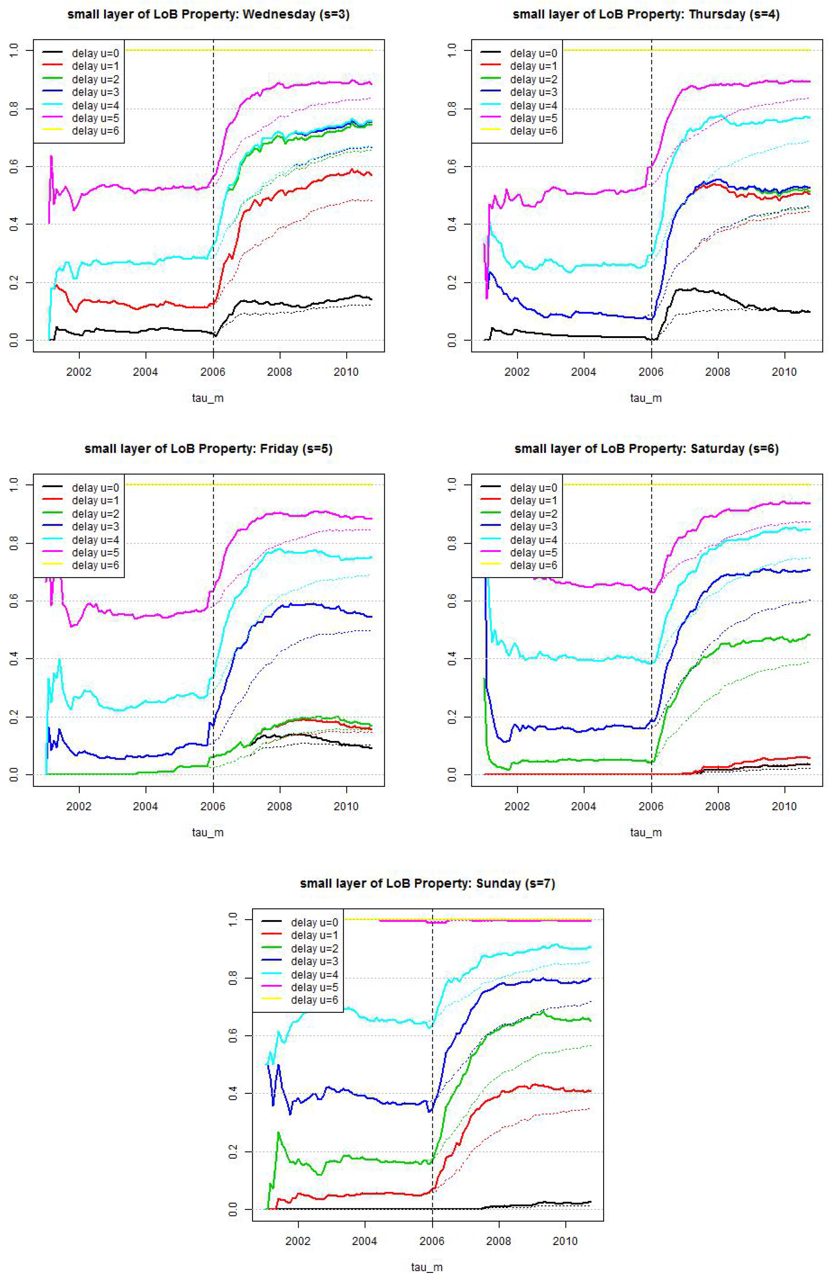
We start by considering the small reporting delay layer . Data shows that reporting delays have a weekly pattern because claims divisions do not (necessarily) work at weekends and a claim occurring, for instance, on a Saturday can only be reported on Monday. This is illustrated in Figure 6. This indicates that we need a (week-) daily modeling approach. In order to not over-parametrize our model we try to keep this (week-) daily modeling layer as small as possible. The canonical choice then is to set because after one week all claims have experienced a full weekly cycle and reporting should be on a similar level for all weekdays, this is supported by Figure 6 (middle), though not fully.
We could now try to maximize the log-likelihood (15) by brute force. Observe that this includes a coupling between all layers through exposures because we have . This is unpleasant from a computational point of view, and we therefore propose an approximation. For we have which implies for all . For we have from (17) and under Assumption 5, assumption and a change of variable
This shows that if parameter splits into parameters for , , and and (we omit possible time dependence in the notation of and ), then the coupling of the lower layer with the other two layers happens through and and in exposures . If we neglect in (18) the latest 7 days of observations, i.e., claims with occurrence dates , then the calibration of the lower layer density completely decouples from the other two layers because we have full information (no missing data) for accidents with occurrence dates in at time . This is indicated by the dashed red line in Figure 7 (lhs). In most cases this provides a reasonable approximation because the last days will not completely change the calibration of the lower reporting delay distribution if we have observations over, say, 10 years ≈ 3652 days. For this reason we shorten the last time interval to which provides in view of (15) MLE for
where denotes the number of reported claims at time with accident dates and reporting delays . The first component of Θ is assumed to fully characterize density but no other part of the reporting delay distribution.
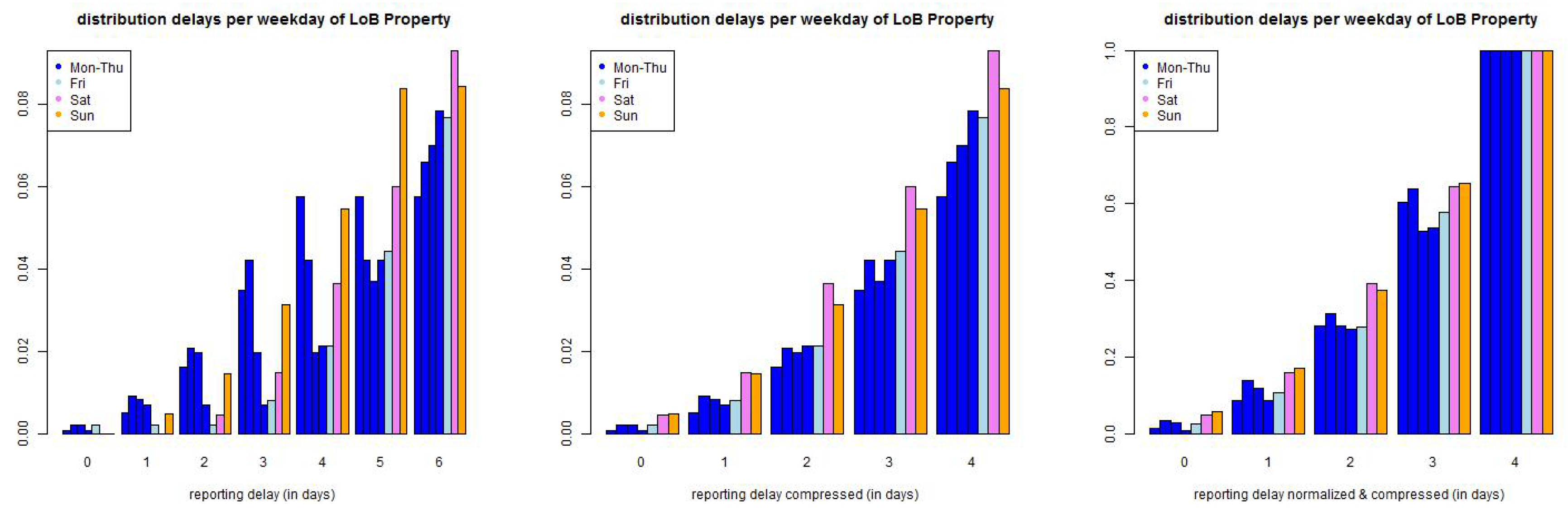
Next we discuss the explicit choice of . In Figure 6 (lhs) we plot the empirical distribution of all claims with accident dates before 01/2006 and a maximal reporting delay of 365 days. Figure 6 only shows the claims with reporting delays , i.e., belonging to the small layer. The lhs shows the individual delay distributions per weekday of occurrence, the middle pictures the same distributions but compressed by the weekends (because there are (almost) no reportings on Saturdays and Sundays) and the rhs shows the compressed graph that is normalized to 1 at time . The graphs indicate that we should start by modeling weekdays individually. We make the following Ansatz: choose discrete distributions with, for and ,
with such that . The second identity in (20) implies that we obtain a weekly periodic reporting delay distribution with 42 parameters , if we assume stationarity (20) on the weekly time grid. We may even ask for more parameters because of potential non-stationarity of the reporting behavior, see Figure 2. We refrain from doing so but we use a rolling window to detect and capture non-stationarity. We should also remark that the 42 parameters raise questions about over-parametrization. We will investigate this question below and we will find that we can reduce the number of parameters in LoB Casualty, in LoB Property we will work with parametrization (20) which will provide rather stable results due to sufficient volume in this LoB.
Optimization problem (19) provides Lagrangian with Lagrange multipliers
The MLE of (19) is then found by setting the derivatives of w.r.t. and χ equal to zero and solving this system of equations. For and we define to be the number of reported claims at time with accident dates in , reported on weekday s and having reporting delay u (we think of being Mondays and being Sundays). The MLE of at time is then given by
The lower reporting delay layer distribution is at time estimated by
To capture potential non-stationarity we will choose a fixed window length K and consider this estimate based on observations in .
5.2.2. Empirics and Fitting the Small Reporting Delay Layer Distributions
We estimate distributions (21) in the lower reporting delay layer for the 2 LoBs.
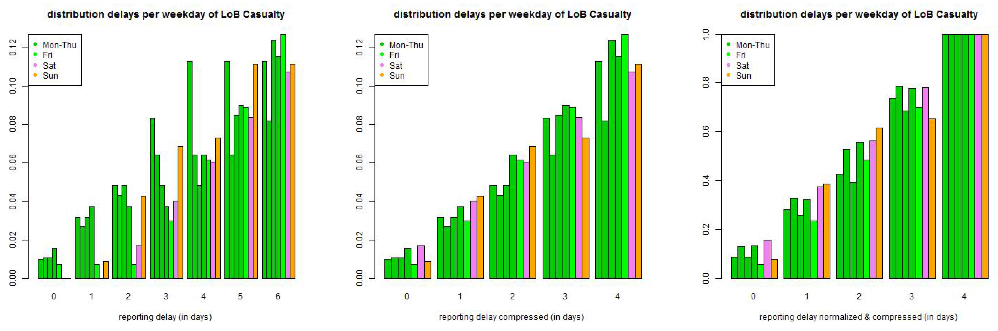
In Table 2 and Table 3 we give the observed number of reported claims for weekdays and reporting delays at time for claims with accident dates before 26/10/2010. We see that there is a weekly pattern with no reportings on weekends in LoB Casualty and fewer reportings on weekends in LoB Property. For the latter we estimate all parameters individually, for the former we may also discuss other approaches, for instance, compressing weekends and shift the weekdays in Table 3 to the left (which is done on the rhs of Table 3). Moreover, the numbers in Table 3 are rather small and of similar size which may also suggest that we should not distinguish different reporting delays. We investigate this more formally below.
We start with LoB Property. We show in Figure 8 the resulting estimates (see (20)) with a rolling window of length 2·365 days (solid lines) which is compared to the estimate considering all observations (dotted lines). We clearly see the non-stationarity after the break point at 1/1/2006, and the rolling window seems to capture it rather well. Therefore, we do not use any other measures here, but work with the rolling window of length 2·365 days (solid lines).
For LoB Casualty the non-stationarity is less obvious, see Figure 9. In fact, the resulting estimates with a rolling window of length 2·365 days (solid lines) are rather volatile which is a clear sign of over-parametrization. The dotted lines show the estimates based on all available observations, these are much smoother with a slight positive trend for some of the weekdays. At this point we could investigate more thoroughly this non-stationarity, we refrain from doing so because in this case study it may only marginally influence the estimation of the number of IBNYR claims: the potential trend has a very moderate slope which affects less then 10% of the claims in LoB Casualty (small reporting delay layer). For this reason, we simply choose a stationary model and we mainly aim at studying whether we can further reduce the number of parameters in . First, we compress the weekends (in Table 3 we go from the lhs denoted to the rhs denoted ). Then we test the null hypothesis whether for all weekdays and compressed reporting delays we can choose the same (empirical) probability, and for all weekdays we can choose the same probability for reporting delay , that is, we test the null hypothesis (delay does not differ between weekdays ) and (delays and weekdays do not differ). We perform for every weekday a Pearson’s -test (for the information at time ). The corresponding test statistics is
with being the number of reported claims with occurrence day s and compressed reporting delay , and being the corresponding MLE under the null hypothesis.
We provide the resulting p-values in Table 4. The resulting p-value for claims with accident dates on Wednesdays is 3.2% and for all other weekdays s we obtain p-values bigger than 20%. We consider these p-values to be sufficiently large so that we do not reject the null hypothesis. This leads to a substantial reduction in the number of parameters, and we only choose three different values for at any time point in this reduced case (the third one being 0% for weekends). In Figure 10 we show the results, the solid line gives the estimates under the null hypothesis and the dotted lines the estimates of the model with 42 parameters. For LoB Casualty we choose this reduced model (under the null hypothesis).
Using (18) and the fact that we choose a step function for we obtain estimated probability in the small reporting delay layer given by
The results are presented in Figure 4 and they are compared to the case where we do not choose a weekly periodic pattern, that is, where we set . This latter model is the one used in Section 4.2 of Antonio-Plat [17]. We see that the weekly periodic pattern essentially smooths the estimates, in particular, for weekends in LoB Casualty. This confirms the findings of Section 4.3 and, in particular, of Figure 5. For this reason we continue with the model allowing us for the modeling of a weekly periodic pattern . We fix the resulting estimates and then calibrate the middle and large layers, this is explained next.
5.3. Calibration of Middle and Large Reporting Delay Layers
We come back to log-likelihood (15). We replace in the small reporting delay layer parameter by its estimate derived in the previous subsection. This provides the log-likelihood at time , we only show the terms including the unknown parameters ,
where for . From this we compute the MLE of (see also Lemma 3):
If we insert this back into (24) we get (only stating relevant terms for parameter estimation)
where we have used Assumption 5 for with . Recall that we have normalization of the layer probabilities because the reporting delays need to be in one of the three layers. Assuming we can normalize these probabilities by dividing by this third probability and setting . From this we see that we can rewrite the last log-likelihood in terms of . This provides the log-likelihood
To implement MLE of (26) there remains the calculation of for . This is what we are going to discuss next.
5.3.1. Choice of Layers and Approximate Log-likelihood
We still need to specify threshold . The lower limit was chosen to be days. For we test different reporting delays or 12 months. Note that κ months is not well-defined in terms of number of days. We set equal to or 365 which is the minimal number of days that κ consecutive calendar months can have. The accident periods with are then fully observed in the middle layer at time , and we have
Thus, we only need to study in more detail for the middle reporting delay layer. As for the large reporting delay layer we see that there are no observations possible at time for accident periods with and, therefore,
The remaining layers and probabilities are more involved, and we consider these next.
Large reporting delay layer with . For we have under Assumption 5
To simplify optimization (26) we assume that for reportings in the large layer the weekly periodic pattern only has a marginal influence. This is justified by the argument that between claims occurrence and reporting there are at least κ months of delay, and therefore the specific weekday of the accident should only marginally influence the late reporting (as long as a particular claim type cannot only occur on one specific weekday). For this provides the approximation
The situation is more delicate. We have which is the minimal number of days that κ consecutive calendar months can have, the maximal number of days being or 366 days, respectively. Therefore, the following integral may also be non-zero on time interval at time
Note that and which implies that for all m. Therefore, this term only marginally influences the results (and it could also be skipped for parameter estimation but we will keep it).
Middle reporting delay layer with . We still need to treat the cases and . We have for
As we indicate below, this can be implemented and MLE can be performed. In order to speed up the MLE optimization we also approximate . However, this approximation is only used for parameter estimation, for the number of IBNYR claims estimation we will use the exact form . For the approximation in MLE we also neglect weekday differences which provides for
For we have for . This provides the approximation
because otherwise reporting delays belong to the small layer.
This allows us to approximate the log-likelihood (26) by (we also refer to Corollary 7, below)
where several of the π’s and ’s are either 0 or 1 (we give them in detail below). To calculate them we need the following lemma.
Lemma 6.
Assume and choose . We have
Proof of Lemma 6.
The proof follows by applying integration by parts. ☐
Corollary 7.
We choose and denote the corresponding expectation by .
- Small layer . For we have probability and the case is given by (23).
- Middle layer . For we have probability . For we haveand for
- Large layer . For we have probability . For we haveand for
Finally, we need to choose explicit distribution functions for the reporting delay layers . This is what we are going to do in the next subsection.
5.3.2. Choice of Explicit Distributions and Layer Probabilities
There remains the modeling of the reporting delay distributions in the middle and large layers as well as the relative layer probabilities for . We have considered different models, compared them to each other, checked them for robustness and applied statistical model selection criteria such as Akaike’s information criterion. Our favorite model that is at the same time not too difficult and gives appropriate results is the following: (i) for the middle layer we choose a stationary truncated log-normal distribution, (ii) for the upper layer we choose a stationary shifted log-normal distribution, and (iii) we choose non-stationary relative layer probabilities . We justify these choices by some statistical analysis below.
Lemma 8.
Assume has a truncated log-normal distribution with parameters and supported in a non-empty interval . The density of is given by
The distribution of is given by
The expectation of on layer is given by
Assume has a shifted log-normal distribution with Z being log-normally distributed with parameters and . We have on the layer , set and ,
Proof of Lemma 8.
The proof is a straightforward consequence of calculations with log-normal distributions, see also Section 3.2.3 in [21]. ☐
The model of Lemma 8 will be chosen below. We will compare it to the situation where we also have a truncated log-normal distribution for in the upper layer, and we also compare it to the case of replacing the log-normal by gamma distributions. More details are provided below.
There remains the choice of for . We consider for break point , and the functional forms
with given trend parameter after break point . For we have
This shows that we roughly model a γ-power increase/decrease after the break point . Normalization implies
This shows that is almost constant for α small, i.e., the break point only marginally influences late reportings (because it mainly speeds up immediate reporting after claims occurrence, this will be seen below and corresponds to the red graphs in Figure 11).
With these choices we revisit log-likelihood (27) which is now given by, set ,
If we use the explicit truncated/translated log-normal distributions introduced in Lemma 8 there are 9 parameters involved in this optimization. Note that we use canonical translation for the upper layer distribution .
5.3.3. Preliminary Model Selection
We need to choose optimal parameters for the model presented in Lemma 8. This can be achieved by applying MLE to log-likelihood (29). Since, eventually, we would like to do this for any time point , this would be computationally too expensive, and also not sufficiently robust (over time). For this reason we do a preliminary model selection based on the data as of 31/10/2010. In this preliminary model selection analysis we determine (a) the explicit distributions, (b) the upper layer threshold as well as (c) the parameter of power function (28). Based on these three choices we then calibrate the model for the time series . These three choices are done based on Table 5, Table 6 and Table 7.
We start by comparing the following models for the pair : (i) truncated/shifted log-normal (as in Lemma 8); and (ii) truncated/truncated log-normal. For these two models we consider the static version in (28) and the dynamic version . We set and months (this is further considered below) and then we calculate the MLE of , , (for the static version) and the MLE of (for the dynamic version). Finally, we calculate Akaike’s information criterion (AIC) and the Bayesian information criterion (BIC) for these model choices. The model with the smallest AIC and BIC, respectively, should be preferred. The results are presented in Table 5 (top). LoB Property: the dynamic () truncated/truncated log-normal model should be preferred, closely followed by the dynamic () truncated/shifted log-normal one. LoB Casualty: the truncated/truncated log-normal model should be preferred, the static and the dynamic versions are judged by BIC rather similarly. We have decided in favor of the static version because this reduces the number of parameters to be selected.
Next we analyze AIC and BIC of the optimal layer limit for the dynamic truncated/truncated log-normal model in LoB Property (for given ) and the static truncated/truncated log-normal model in LoB Casualty. The results are presented in Table 5 (bottom). We observe that we prefer for both LoBs a small threshold of months.
Next we do the same analysis for the parameter γ in the dynamic () version of LoB Property, see Table 6 and we compare the log-normal model to the gamma model, see Table 7. From this preliminary analysis our conclusions are:
- ⊳
- LoB Property: We choose the dynamic () truncated/truncated log-normal model with and months.
- ⊳
- LoB Casualty: We choose the static () truncated/truncated log-normal model with months.
These are our preferred models as of and the remaining model parameters are obtained by MLE from (29).
5.3.4. Model Calibration Over Time
In the previous subsection we have identified the optimal models as of using AIC and BIC. Observe that this is the optimal model selection with having maximal available data. This selection will be revised in this subsection because we study the models when incoming information increases over . In Figure 12 and Figure 13 we present the MLEs of parameters using (29) for (lhs) the truncated/truncated log-normal models and (rhs) the truncated/shifted log-normal models. LoB Property considers the dynamic version with and LoB Casualty considers the static version . From this analysis we see that the parameters behave much more robust over time in the truncated/shifted log-normal model, see Figure 12 (rhs) and Figure 13 (rhs). For this reason we abandon our previous choice, and we select the truncated/shifted log-normal model for both LoBs. This is in slight contrast to the AIC and BIC analysis in the previous subsection, but the differences between the two models in Table 5 (lhs) are rather small which does not severely contradict the truncated/shifted model selection. In addition, for LoB Property we choose threshold months (Figure 12 (top, rhs)) and for LoB Casualty we decide for the bigger threshold months (Figure 13 (bottom, rhs)), also because estimation over time is more robust for this latter choice.
In Figure 11 we provide the estimated layer probabilities , , in the truncated/shifted log-normal model for LoB Property (with months) and for LoB Casualty (with months) for . The solid lines give the dynamic versions with and the dotted lines the static versions . In LoB Property we observe stationarity of these layer probabilities up to break point , and our modeling approach Equation (28) with seems to capture the non-stationarity after the break point rather well (note that the thin solid line shows an exact function after the break point by considering the map at time and the dotted lines show the stationary case ). In this analysis we also see that LoB Casualty may be slightly non-stationary after 1/1/2008, see Figure 11 (rhs). This was not detected previously, but is also supported by the time series of the trend parameter α estimates given in Figure 7 (rhs). However, since the resulting trend parameter α is comparably small we remain with the static version for LoB Casualty.
Our conclusions are as follows. For LoB Property we choose the dynamic () truncated/shifted log-normal model with and months; for LoB Casualty we choose the static () truncated/shifted log-normal model with months. In Figure 14 we present the resulting calibration as of . In the middle layer the fitted distribution looks convincing, see Figure 14 (top). In the upper layer the fitted distribution is more conservative than the observations, see Figure 14 (bottom), this is supported by the fact that the empirical distribution is not sufficiently heavy-tailed because of missing information about late reportings (IBNYR claims in upper left triangles in Figure 2). This missing information has a bigger influence in casualty insurance because reporting delays are more heavy-tailed. Moreover, in both LoBs the shifted modeling approach is more conservative than the truncated one.
The model is now fully specified and we can estimate the number of IBNYR claims (late reportings). Using Equations (6), (25) and replacing all parameters Θ by their MLEs at time we receive estimate for the total number of incurred claims in time interval
The number of estimated IBNYR claims is given by the difference . For illustration we choose three time points , and we always use the relevant available information at those time points . The results are presented in Figure 15, the blue/green line gives the number of reported claims and the red line the estimated number of incurred claims (the spread being the number of estimated IBNYR claims). We note that the spread is bigger for LoB Casualty than LoB Property (which is not surprising in view of our previous analysis). For LoB Property in Figure 15 (top) we also compare the static (gray) to the dynamic (red) estimation. The static version seems inappropriate since it cannot sufficiently capture the non-stationarity and estimation is too conservative after the break point .
In the final section of this paper, we back-test our calibration and estimation, and compare it to the chain-ladder estimation.
6. Homogeneous (Poisson) Chain-Ladder Case and Back-Testing
In this section we compare our individual claims modeling calibration to the classical chain-ladder method on aggregate data. The chain-ladder method is probably the most popular method in claims reserving. Interestingly, the cross-classified chain-ladder estimation can be derived under Model Assumptions 2 and additional suitable homogeneity assumptions.
6.1. Cross-Classified Chain-Ladder Model
We choose an equidistant grid
Denote by the number of claims with accident dates in and reporting dates in , for and . Under Model Assumptions 2 the random variables are independent and Poisson distributed with exposures
We now make the following homogeneity assumptions for and
i.e., we may drop time index t in and , respectively. We define . Assumptions (31) imply
If we now define reporting pattern by
we see that under (31) the random variables are independent and Poisson distributed with
Moreover, we have normalization . This provides the cross-classified Poisson version of the chain-ladder model. Under the additional assumption that for a finite J the MLE exactly provides the chain-ladder estimator. This result goes back to Hachemeister-Stanard [22], Kremer [23] and Mack [24], and for more details and the calculation of the chain-ladder estimator of with at time we refer to Theorem 3.4 in Wüthrich-Merz [25]. Using these chain-ladder estimators we get estimate
for the estimated number of claims in period with . This chain-ladder estimate is compared to the estimate provided in (30).
6.2. Back-Testing
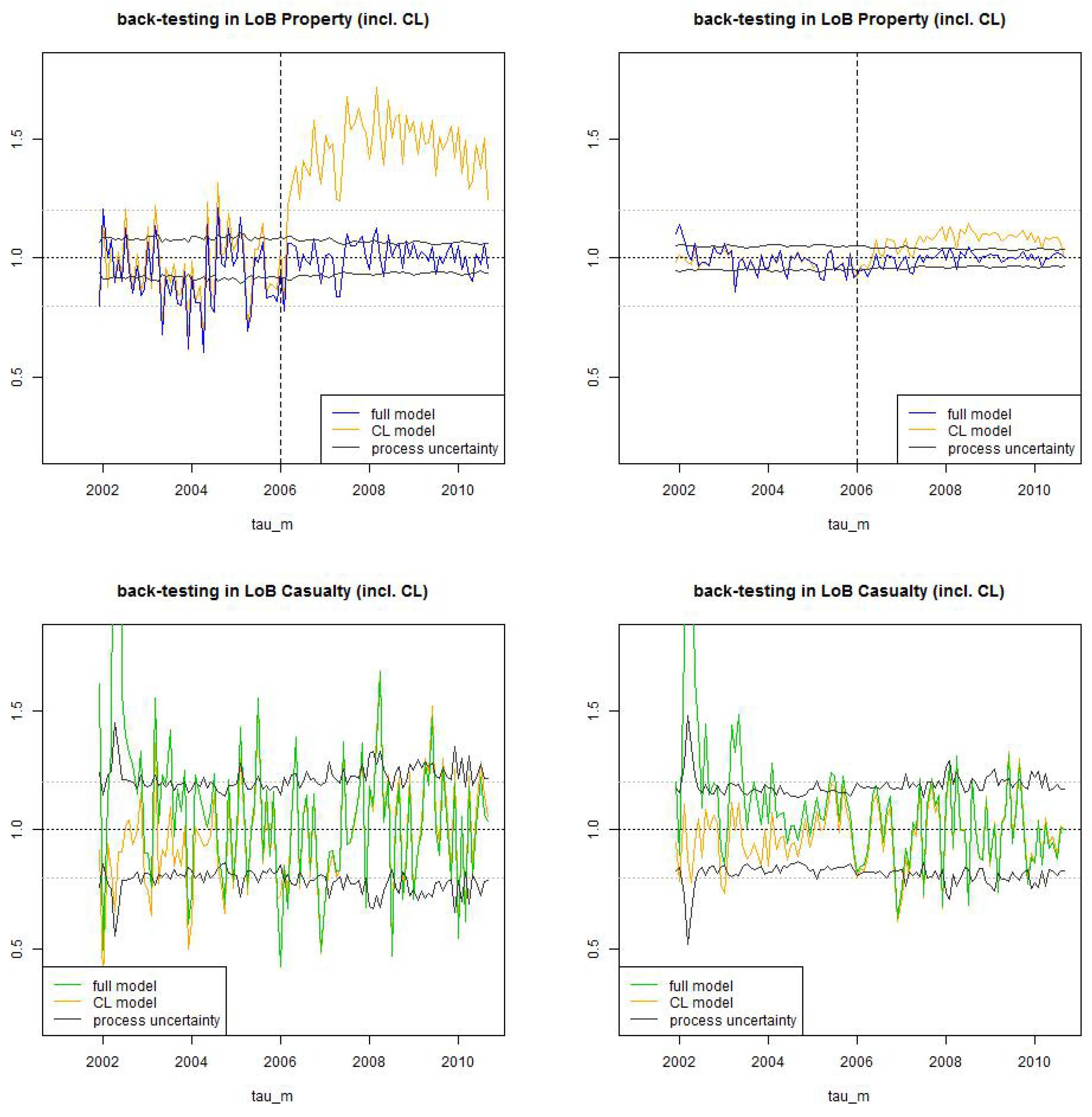
In this section we back-test the estimations obtained by calibration (21) and (29) and compare it to the homogeneous chain-ladder case (33). We therefore calculate for each exposure period with the estimates and . These estimates are compared to the latest estimates and at time . In particular, we back-test the estimates with time lags against the latest available estimation. We therefore define the ratios
The first ratio compares the estimation of the number of claims in period based on the information available at time to the latest available estimation at time , and the second variable considers the same ratio but with the estimation based on the information at time (i.e., after one period of development). Moreover, we calculate the relative process uncertainties for defined by
this is the relative standard deviation of the number of IBNYR claims at time for a Poisson random variable, normalized with to make it comparable to . We present the results in Figure 16:
- Figure 16 (top), LoB Property: We see that the chain-ladder estimate , , clearly over-estimates the number of claims after the break point , whereas our non-stationary approach (28) can capture this change rather well and estimations are centered around 1. Remarkable is that after 5 years of observations, the volatility of the estimation can almost completely be explained by process uncertainty (we plot confidence bounds of ), which means that model uncertainty is comparably low. We also see that the faster reporting behavior after break point has substantially decreased the uncertainty and the volatility in the number of IBNYR claims. Before the break point, uncertainty for is comparably high, this can partly be explained by the fact that claims history is too short for model calibration.
- Figure 16 (bottom), LoB Casualty: After roughly 5 years of claims experience the estimation in the individual claims model and the chain-ladder model are very similar. This indicates that in a stationary situation, the performance of the (simpler) chain-ladder model is sufficient. However, this latter statement needs to be revised because non-stationarity can be detected more easily in the individual claims history modeling approach, in particular, the individual claims model reacts more sensitively to structural changes. The confidence bounds have a reasonable size because the back-testing exercise does not violate them too often (i.e., the observations are mostly within the confidence bounds), however, in practice they should be chosen slightly bigger because they do not consider model uncertainty.
We close this section with a brief discussion of two related modeling approaches. Our approach can be viewed as a refined model of the one used in Antonio-Plat [17]. The first refinement we use is that we consider the weekly periodic pattern which was supported by the statistical analysis given in Figure 5. Neglecting this weekly periodic pattern would lead to less smooth small layer probabilities, in particular, in LoB Casualty, see Figure 4. The second refinement is that we choose a reporting delay distribution that depends on the weekday of the claims occurrence. This is especially important for the small reporting delay layer because weekday configuration essentially influences the short reporting delays. In our analysis, this then leads to a mixture model with three different layers. Antonio-Plat [17] use a mixture of a Weibull distribution and 9 degenerate components which fits their purposes well. Our approach raises the issue of over-parametrization which we analyze graphically, i.e., we observe rather stable parameter estimates after 4 years of observations, see for instance Figure 12 (rhs) and Figure 13 (rhs).
The issue of over-parametrization is of essential relevance if we would like to do prediction for future exposure periods. That is, in our analysis we have mainly concentrated on making statistical inference of the instantaneous claims frequency of past exposures at a given time point . Going forward, we may also want to model and predict the claims occurrence and the claims reporting processes, respectively, of future exposures. An over-parametrized model will have a low predictive power because it involves too much model uncertainty, therefore we should choose as few parameters as necessary. Moreover, for predictive modeling it will also be necessary to model stochastically the instantaneous claims frequency process Λ, i.e., our statistical inference method is not sufficient for predicting claims of future exposures, but it will help to calibrate a stochastic model for Λ. A particularly interesting model is the marked Cox model proposed in Badescu et al. [18,19]. Similarly to Antonio-Plat [17], Badescu et al. [18,19] consider the piece-wise homogeneous case (7), but with being a state-dependent process which is driven by a time-homogeneous hidden Markov process (in the sense of a state-space model). We believe that this is a promising modeling approach for claims occurrence and reporting prediction, if merged with our weekday dependent features (both for claims occurrence and claims reporting delays).
6.3. Conclusions
We have provided an explicit calibration of a reporting delay model to individual claims data. For the two LoBs considered it takes about 5 years of observations to have sufficient information to calibrate the model (this is true for the stationary case and needs to be analyzed in more detail in a non-stationary situation). As long as the claims reporting process is stationary the individual claims reporting model and the aggregate chain-ladder model provide very similar estimates for the number of IBNYR claims, but as soon as we have non-stationarity the chain-ladder model fails to provide reliable estimates and one should use individual claims modeling. Moreover, our individual claims modeling approach is able to detect non-stationarity more quickly than the aggregate chain-ladder method. Going forward, there are two different directions that need to be considered. First, for the evaluation of parameter uncertainty one can embed our individual claims reporting model into a Bayesian framework (this is similar to the Cox model proposed in Badescu et al. [18,19]) or one can use bootstrap methods. Secondly, the far more difficult problem is the modeling of the cost evolution and the claims cash flow process. We believe that this is still an open problem and it is the next building block of individual claims reserving that should be studied on real data examples.
Author Contributions
Both authors have contributed equally to this paper.
Conflicts of Interest
The author declares no conflict of interest.
Appendix A. Proofs
Proof of Lemma 3.
We maximize likelihood function (9). The derivatives of its logarithm provide for the requirements (denoted by )
and for the derivative w.r.t. the reporting delay parameter Θ we obtain
The first requirements provide identity
Plugging this into the second requirement provides identity
where in the last identity we have added constants in Θ which vanish under the derivative (note that these constants were added to indicate that we obtain the densities (10)). ☐
Proof of Lemma 4.
We maximize likelihood function (9) for on weekly time grid under side constraint and under assumption (11) which implies and for . The corresponding Lagrangian is given by
Under the above assumptions we calculate the derivative w.r.t. , , of the Lagrangian
and the derivative w.r.t. are given by
where we have used on the weekly time grid . The latter implies and plugging this into the former requirement provides
This implies that
Lagrange multiplier χ is found from normalization which provides the claim. ☐
References
- W.S. Jewell. “Predicting IBNYR events and delays I. Continuous time.” ASTIN Bull. 19 (1989): 25–55. [Google Scholar] [CrossRef]
- W.S. Jewell. “Predicting IBNYR events and delays II. Discrete time.” ASTIN Bull. 20 (1990): 93–111. [Google Scholar] [CrossRef]
- H. Bühlmann, R. Schnieper, and E. Straub. “Claims reserves in casualty insurance based on a probabilistic model.” Bull. Swiss Assoc. Actuaries 1980 (1980): 21–45. [Google Scholar]
- E. Arjas. “The claims reserving problem in non-life insurance: Some structural ideas.” ASTIN Bull. 19 (1989): 139–152. [Google Scholar] [CrossRef]
- R. Norberg. “Prediction of outstanding liabilities in non-life insurance.” ASTIN Bull. 23 (1993): 95–115. [Google Scholar] [CrossRef]
- R. Norberg. “Prediction of outstanding liabilities II. Model variations and extensions.” ASTIN Bull. 29 (1999): 5–25. [Google Scholar] [CrossRef]
- S. Haastrup, and E. Arjas. “Claims reserving in continuous time; a nonparametric Bayesian approach.” ASTIN Bull. 26 (1996): 139–164. [Google Scholar] [CrossRef]
- G. Taylor. The Statistical Distribution of Incurred Losses and Its Evolution Over Time I: Non-Parametric Models. Arlington, VA, USA: Casualty Actuarial Society, 1999, working paper. [Google Scholar]
- G. Taylor. The Statistical Distribution of Incurred Losses and Its Evolution Over Time II: Parametric Models. Arlington, VA, USA: Casualty Actuarial Society, 1999, working paper. [Google Scholar]
- T. Herbst. “An application of randomly truncated data models in reserving IBNR claims.” Insur. Math. Econ. 25 (1999): 123–131. [Google Scholar] [CrossRef]
- C.R. Larsen. “An individual claims reserving model.” ASTIN Bull. 37 (2007): 113–132. [Google Scholar] [CrossRef]
- G. Taylor, G. McGuire, and J. Sullivan. “Individual claim loss reserving conditioned by case estimates.” Ann. Actuar. Sci. 3 (2008): 215–256. [Google Scholar] [CrossRef]
- A.H. Jessen, T. Mikosch, and G. Samorodnitsky. “Prediction of outstanding payments in a Poisson cluster model.” Scand. Actuar. J. 2011 (2011): 214–237. [Google Scholar] [CrossRef]
- S. Rosenlund. “Bootstrapping individual claims histories.” ASTIN Bull. 42 (2012): 291–324. [Google Scholar]
- M. Pigeon, K. Antonio, and M. Denuit. “Individual loss reserving with the multivariate skew normal framework.” ASTIN Bull. 43 (2013): 399–428. [Google Scholar] [CrossRef]
- T. Agbeko, M. Hiabu, M.D. Martínez-Miranda, J.P. Nielsen, and R. Verrall. “Validating the double chain ladder stochastic claims reserving model.” Variance 8 (2014): 138–160. [Google Scholar]
- K. Antonio, and R. Plat. “Micro-level stochastic loss reserving for general insurance.” Scand. Actuar. J. 2014 (2014): 649–669. [Google Scholar] [CrossRef]
- A.L. Badescu, X.S. Lin, and D. Tang. “A marked Cox model for the number of IBNR claims: Theory.” Insur. Math. Econ. 69 (2016): 29–37. [Google Scholar] [CrossRef]
- A.L. Badescu, X.S. Lin, and D. Tang. A Marked Cox Model for the Number of IBNR Claims: Estimation and Application. Version 14 March 2016; Rochester, NY, USA: SSRN, 2016. [Google Scholar]
- D.V. Hinkley. “On the ratio of two correlated normal random variables.” Biometrika 56 (1969): 635–639. [Google Scholar] [CrossRef]
- M.V. Wüthrich. Non-Life Insurance: Mathematics & Statistics. Version 15 April 2016; Rochester, NY, USA: SSRN, 2016. [Google Scholar] [CrossRef]
- C.A. Hachemeister, and J.N. Stanard. “IBNR claims count estimation with static lag functions.” ASTIN Colloq., 1975. [Google Scholar]
- E. Kremer. Einführung in die Versicherungsmathematik. Göttingen, Germany: Vandenhoek & Ruprecht, 1985. [Google Scholar]
- T. Mack. “A simple parametric model for rating automobile insurance or estimating IBNR claims reserves.” ASTIN Bulletin 21 (1991): 93–109. [Google Scholar] [CrossRef]
- M.V. Wüthrich, and M. Merz. Stochastic Claims Reserving Manual: Advances in Dynamic Modeling. Version 21 August 2015; Swiss Finance Institute Research Paper No. 15-34; Rochester, NY, USA: SSRN, 2015. [Google Scholar] [CrossRef]
Figure 1.
Observed claims counts from 1/1/2001 until 31/10/2010: (top) LoB Property colored blue and (bottom) LoB Casualty colored green. The lhs gives daily claims counts and the rhs monthly claims counts; the red lines are the rolling averages over 30 days on the lhs and over 2 months on the rhs; violet dots show claims occurrence on Saturdays and orange dots claims occurrence on Sundays, the resulting statistics are provided in Table 1.
Figure 2.
Observed and reported claims counts from 1/1/2001 until 31/10/2010: (top) LoB Property colored blue and (bottom) LoB Casualty colored green. The lhs gives daily claims reporting; the red lines are the 30 days rolling averages; violet dots show claims reporting on Saturdays and orange dots claims reporting on Sundays. The rhs plots accident dates versus reporting delays ; the upper-right (white) triangle corresponds to the missing data (IBNYR claims); the blue/green dots illustrate reported and settled claims; the orange dots reported but not settled (RBNS) claims.
Figure 3.
Box plots of the logged reporting delays on the yearly scale (lhs) LoB Property, (rhs) LoB Casualty.
Figure 3.
Box plots of the logged reporting delays on the yearly scale (lhs) LoB Property, (rhs) LoB Casualty.
Figure 4.
Estimated probability , see (23), for using weekly periodic pattern (blue/green) and setting (black) for (lhs) LoB Property under the full model (21), and (rhs) LoB Casualty under the null hypothesis reduced model.
Figure 4.
Estimated probability , see (23), for using weekly periodic pattern (blue/green) and setting (black) for (lhs) LoB Property under the full model (21), and (rhs) LoB Casualty under the null hypothesis reduced model.
Figure 5.
Weekly periodic pattern estimate (top) LoB Property and (bottom) LoB Casualty: (lhs) time series as a function of and (rhs) for maximal such that (11) holds at time for a maximal reporting delay of 2 years (LoB Property) and of 4 years (LoB Casualty). The confidence bounds in all plots are given by (12) for confidence level .
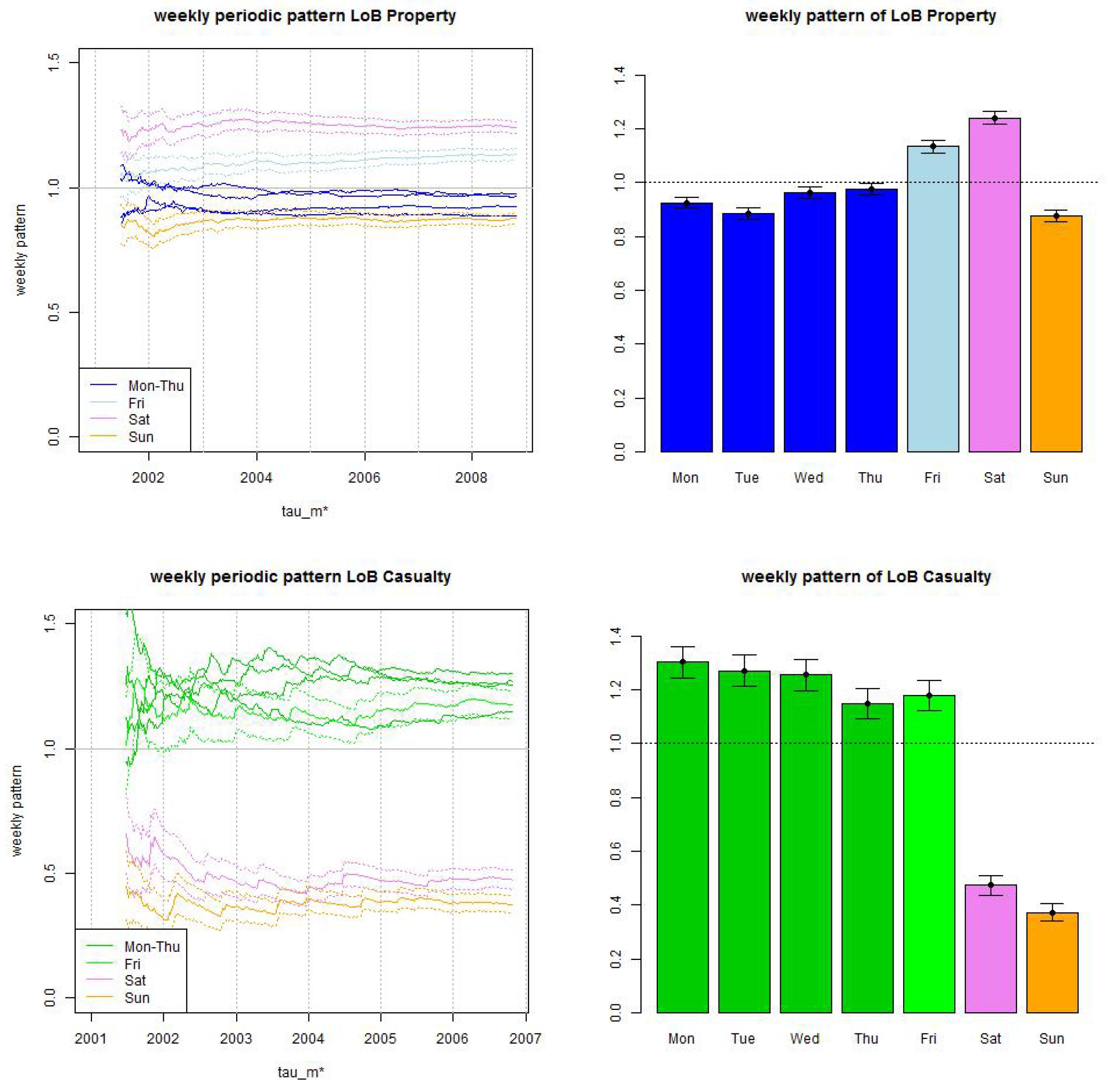
Figure 6.
(top) LoB Property and (bottom) LoB Casualty: empirical distribution of reporting delays separated by weekdays of claims occurrence of all data with accident date prior to 01/2006 and maximal reporting delay of days (lhs) per day, (middle) compressed by weekends, and (rhs) compressed and normalized to 1 after a delay of one week.


Figure 7.
(lhs) small reporting delay layer as of 31/10/2010 for occurrence dates in 10/2010 of LoB Property, and (rhs) estimated trend parameter α at times for LoB Property (blue/light blue) and LoB Casualty (green/light green) with dark colors are for months and light colors for months.
Figure 7.
(lhs) small reporting delay layer as of 31/10/2010 for occurrence dates in 10/2010 of LoB Property, and (rhs) estimated trend parameter α at times for LoB Property (blue/light blue) and LoB Casualty (green/light green) with dark colors are for months and light colors for months.
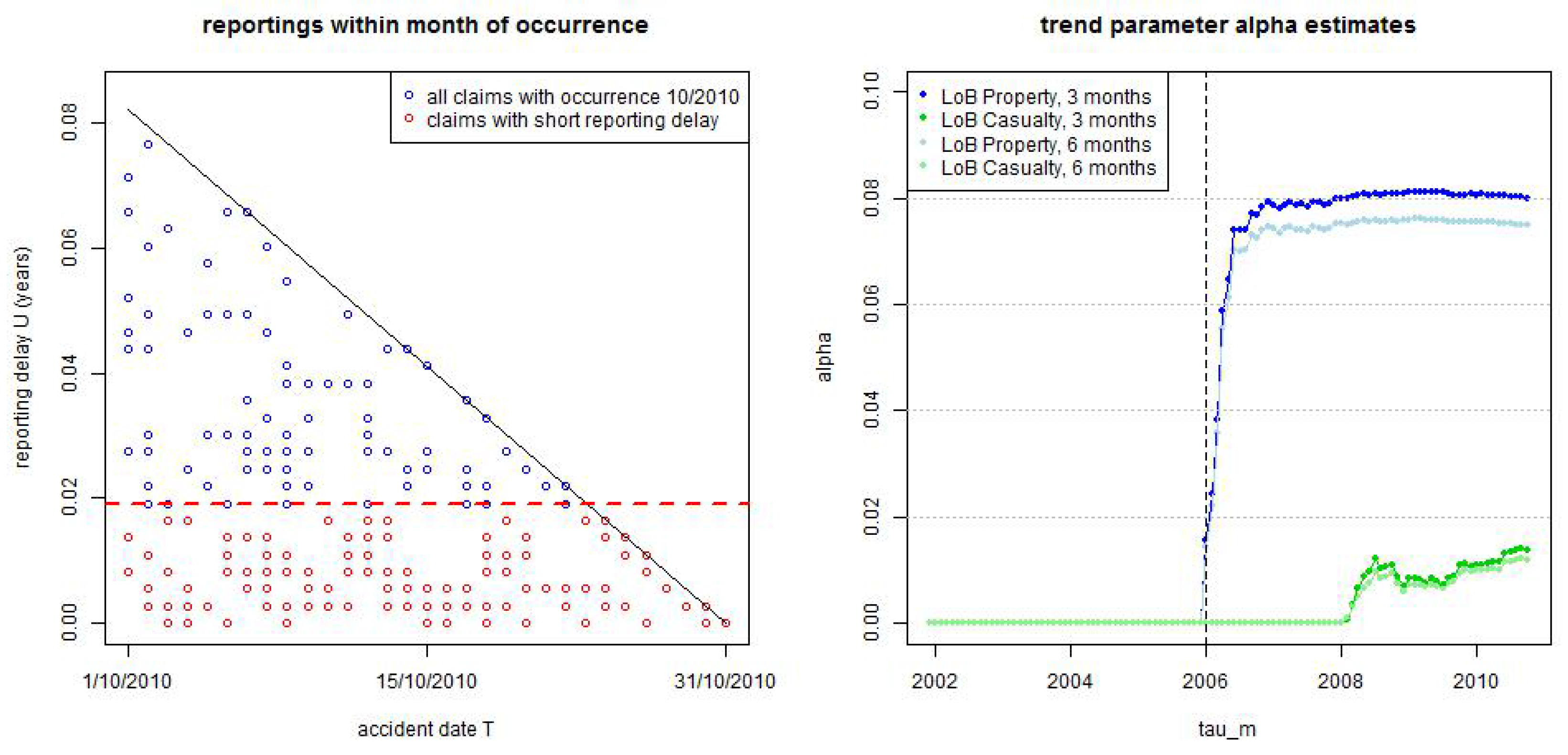
Figure 8.
LoB Property, small reporting delay layer: estimated cumulative distribution per weekday . Dotted lines show calibration based on all observations since and lines show calibration based on a rolling window of length 2·365 days.
Figure 8.
LoB Property, small reporting delay layer: estimated cumulative distribution per weekday . Dotted lines show calibration based on all observations since and lines show calibration based on a rolling window of length 2·365 days.
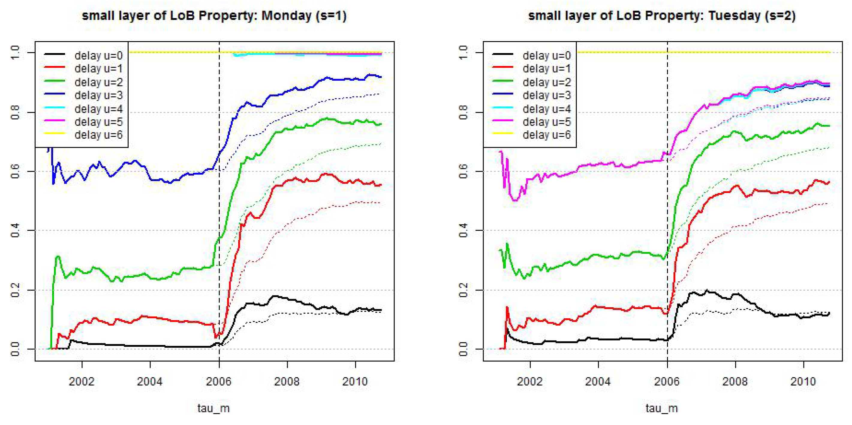

Figure 9.
LoB Casualty, small reporting delay layer: estimated cumulative distribution per weekday . Dotted lines show calibration based on all observations since and lines show calibration based on a rolling window of length 2·365 days.
Figure 9.
LoB Casualty, small reporting delay layer: estimated cumulative distribution per weekday . Dotted lines show calibration based on all observations since and lines show calibration based on a rolling window of length 2·365 days.
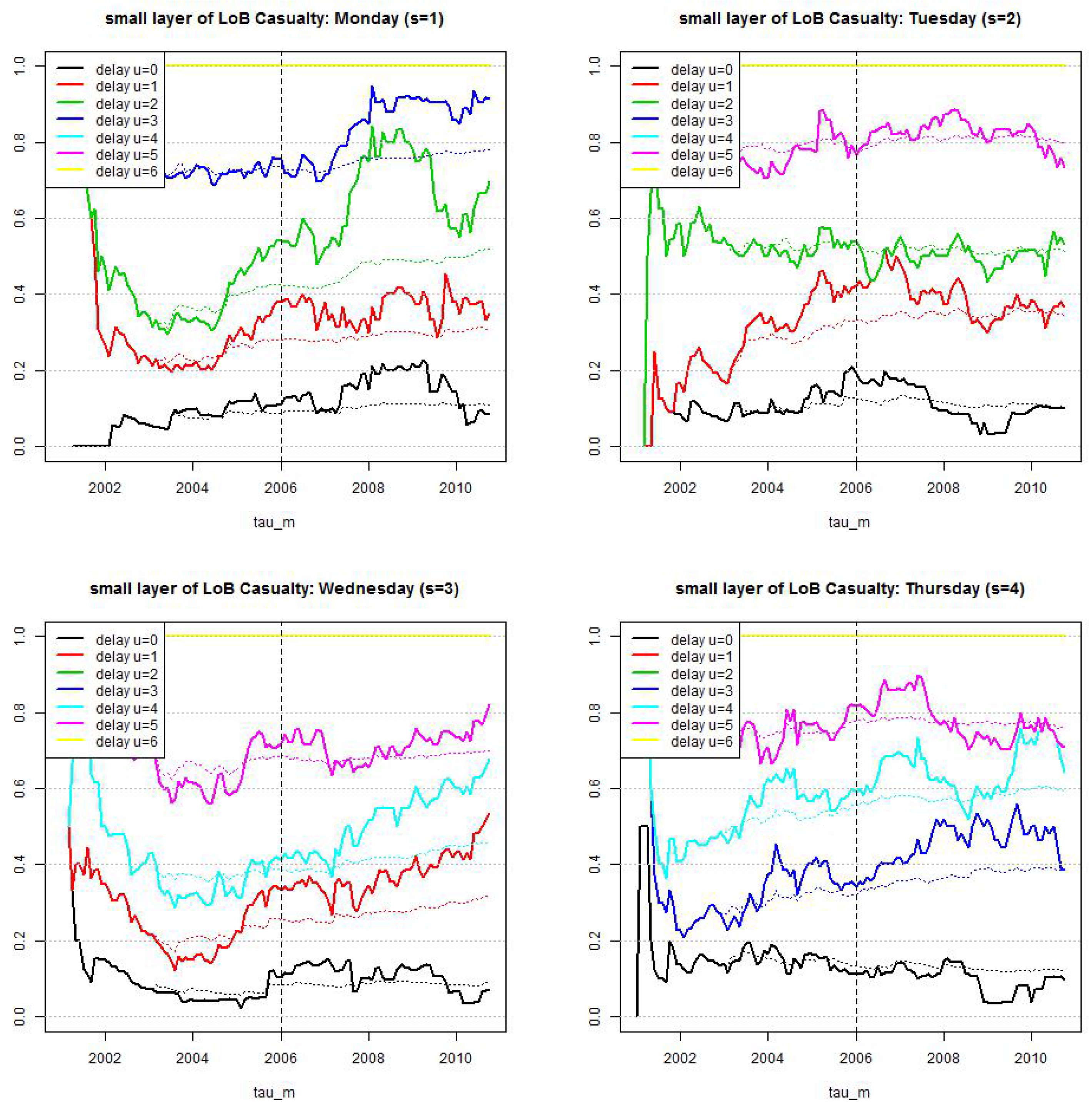
Figure 10.
LoB Casualty, small reporting delay layer: estimated cumulative distribution per weekday . Dotted lines show calibration based on individual weekdays and reporting delays and lines show calibration under compressed weekends and the null hypothesis that we only need three parameters.
Figure 10.
LoB Casualty, small reporting delay layer: estimated cumulative distribution per weekday . Dotted lines show calibration based on individual weekdays and reporting delays and lines show calibration under compressed weekends and the null hypothesis that we only need three parameters.
Figure 11.
Estimated layer probabilities , , in the truncated/shifted log-normal model (lhs) LoB Property with and (rhs) LoB Casualty with months for ; the solid lines give the dynamic versions with and the dotted lines the static versions .
Figure 11.
Estimated layer probabilities , , in the truncated/shifted log-normal model (lhs) LoB Property with and (rhs) LoB Casualty with months for ; the solid lines give the dynamic versions with and the dotted lines the static versions .
Figure 12.
LoB Property: parameter estimates of for the dynamic model with for (top, lhs) months truncated/truncated and (top, rhs) and truncated/shifted; and (bottom, lhs) months truncated/truncated and (bottom, rhs) and truncated/shifted.
Figure 12.
LoB Property: parameter estimates of for the dynamic model with for (top, lhs) months truncated/truncated and (top, rhs) and truncated/shifted; and (bottom, lhs) months truncated/truncated and (bottom, rhs) and truncated/shifted.
Figure 13.
LoB Casualty: parameter estimates of for the static model for (top, lhs) months truncated/truncated and (top, rhs) and truncated/shifted; and (bottom, lhs) months truncated/truncated (bottom, rhs) and truncated/shifted.
Figure 13.
LoB Casualty: parameter estimates of for the static model for (top, lhs) months truncated/truncated and (top, rhs) and truncated/shifted; and (bottom, lhs) months truncated/truncated (bottom, rhs) and truncated/shifted.
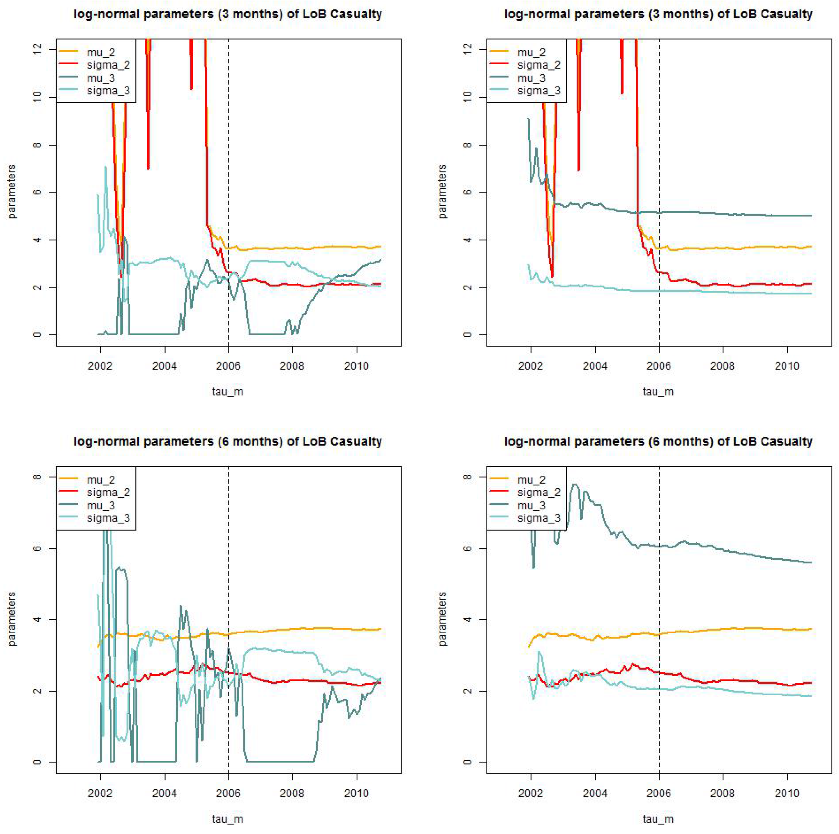
Figure 14.
(top) calibration of truncated log-normal distribution in the middle layer for (lhs) LoB Property with months and (rhs) LoB Casualty with months; (bottom) calibration of shifted and truncated log-normal distributions in the large layer for (lhs) LoB Property with months (static and dynamic versions) and (rhs) LoB Casualty with months (only static versions).
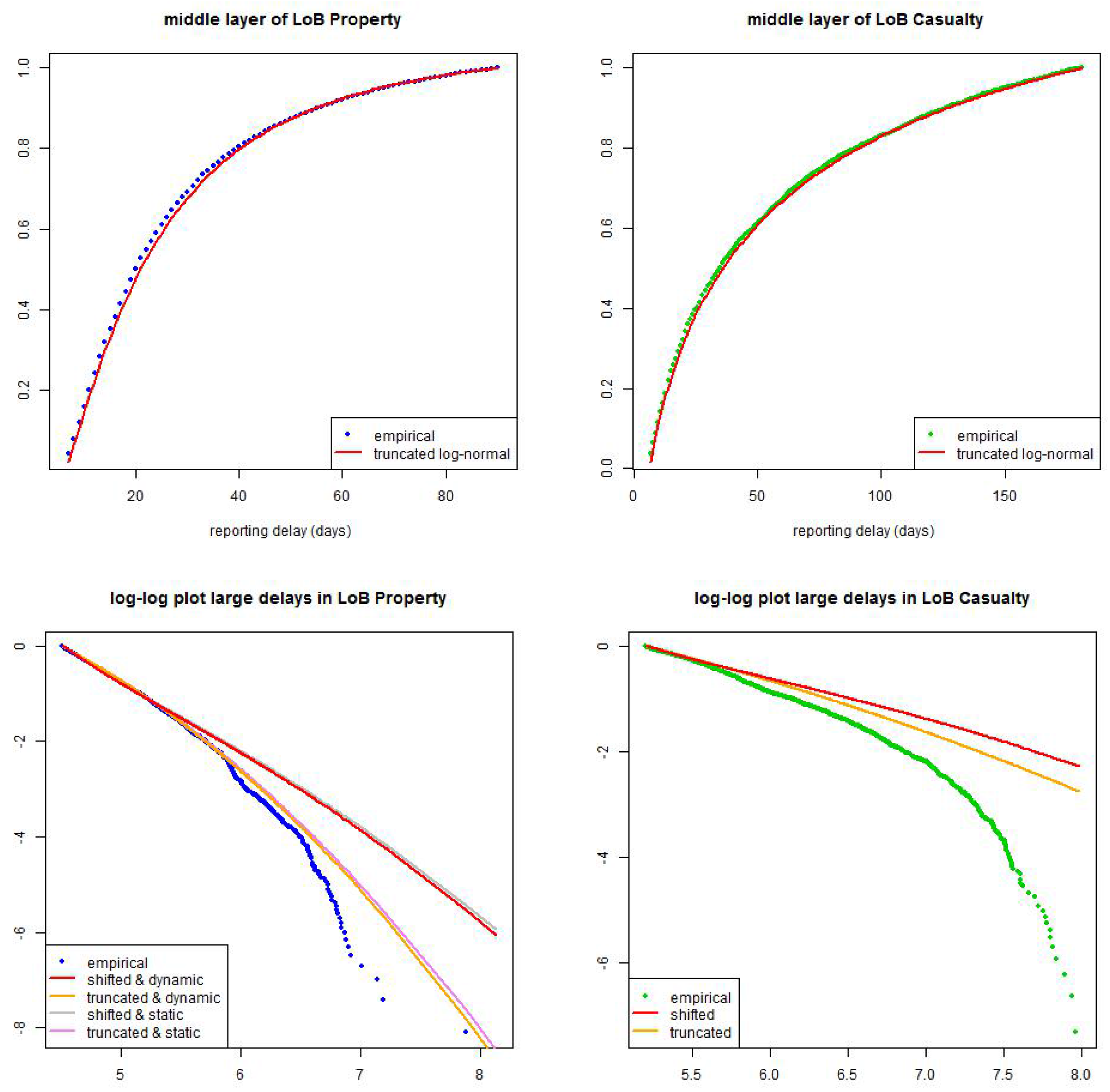
Figure 15.
Estimation of the number of incurred claims for (top) LoB Property and (bottom) LoB Casualty at times using the truncated/shifted log-normal model with months and months, respectively; “observed” (blue/green) gives the number of reported claims in each period at time , “dynamic/static” (red) gives the total number of estimated claims (the spread giving the estimated number of IBNYR claims).
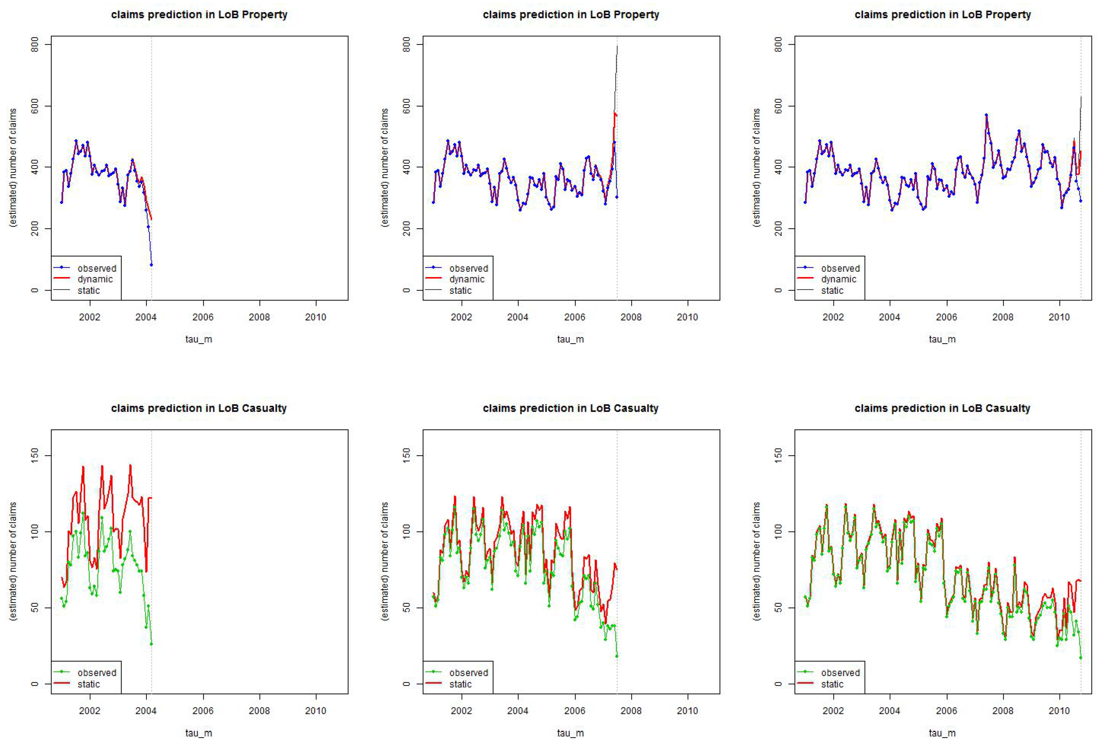
Figure 16.
Back-test LoB Property (top) and LoB Casualty (bottom): we compare the (non-stationary) estimate (blue/green) to the (stationary) chain-ladder estimate (orange) for (lhs) time lag and (rhs) time lag . The black line shows the process uncertainty confidence bounds of 2 (relative) standard deviations .

Table 1.
Statistics per weekday: average daily claims counts and empirical standard deviation for LoB Property and LoB Casualty.
| Mon | Tue | Wed | Thu | Fri | Sat | Sun | |
|---|---|---|---|---|---|---|---|
| LoB Property | |||||||
| average | 11.48 | 11.02 | 11.87 | 12.15 | 14.23 | 15.46 | 10.73 |
| standard deviation | 4.51 | 4.05 | 4.26 | 4.30 | 4.66 | 4.95 | 4.26 |
| LoB Casualty | |||||||
| average | 2.89 | 2.92 | 2.89 | 2.65 | 2.61 | 1.09 | 0.82 |
| standard deviation | 2.72 | 2.82 | 2.63 | 2.40 | 2.45 | 2.08 | 1.80 |
Table 2.
Observed number of reported claims for weekdays and reporting delays at time for claims with accident dates before 26/10/2010 of LoB Property.
| 0 | 1 | 2 | 3 | 4 | 5 | 6 | |
|---|---|---|---|---|---|---|---|
| Mon | 164 | 482 | 254 | 220 | 172 | 5 | 3 |
| Tue | 172 | 504 | 255 | 221 | 3 | 5 | 207 |
| Wed | 178 | 545 | 258 | 17 | 4 | 246 | 248 |
| Thu | 163 | 542 | 20 | 9 | 355 | 239 | 257 |
| Fri | 193 | 88 | 15 | 651 | 369 | 296 | 287 |
| Sat | 49 | 33 | 754 | 445 | 314 | 266 | 266 |
| Sun | 20 | 470 | 307 | 211 | 195 | 197 | 6 |
Table 3.
Observed number of reported claims for weekdays and reporting delays at time for claims with accident dates before 26/10/2010 of LoB Casualty, the rhs is compressed by weekends.
| 0 | 1 | 2 | 3 | 4 | 5 | 6 | 0* | 1* | 2* | 3* | 4* | |
|---|---|---|---|---|---|---|---|---|---|---|---|---|
| Mon | 17 | 31 | 33 | 41 | 34 | 0 | 0 | 17 | 31 | 33 | 41 | 34 |
| Tue | 15 | 36 | 25 | 42 | 0 | 0 | 30 | 15 | 36 | 25 | 42 | 30 |
| Wed | 16 | 40 | 25 | 0 | 0 | 43 | 53 | 16 | 40 | 25 | 43 | 53 |
| Thu | 19 | 43 | 0 | 0 | 33 | 27 | 38 | 19 | 43 | 33 | 27 | 38 |
| Fri | 12 | 0 | 0 | 29 | 40 | 33 | 40 | 12 | 29 | 40 | 33 | 40 |
| Sat | 0 | 0 | 9 | 10 | 12 | 10 | 15 | 9 | 10 | 12 | 10 | 15 |
| Sun | 0 | 5 | 12 | 7 | 5 | 10 | 0 | 5 | 12 | 7 | 5 | 10 |
Table 4.
p-values of the -tests under the corresponding null hypotheses for test statistics , see Equation (22), for weekdays (with 4 degrees of freedom).
| Mon | Tue | Wed | Thu | Fri | Sat | Sun | |
|---|---|---|---|---|---|---|---|
| p-values | 79% | 29% | 3.2% | 37% | 44% | 52% | 47% |
Table 5.
AIC and BIC as of 31/10/2010 (top) and months and (bottom) LoB Property truncated/truncated dynamic () log-normal model with and LoB Casualty truncated/truncated static () log-normal model.
| Method: Log-normal Distribution | AIC | BIC |
|---|---|---|
| LoB Property | ||
| truncated/shifted (static ) | 347’532 | 347’592 |
| truncated/truncated (static ) | 347’461 | 347’522 |
| truncated/shifted (dynamic ) | 339’270 | 339’348 |
| truncated/truncated (dynamic ) | 339’204 | 339’274 |
| LoB Casualty | ||
| truncated/shifted (static ) | 87’979 | 88’028 |
| truncated/truncated (static ) | 87’941 | 87’990 |
| truncated/shifted (dynamic ) | 87’973 | 88’028 |
| truncated/truncated (dynamic ) | 87’934 | 87’990 |
| Threshold | AIC | BIC |
|---|---|---|
| LoB Property | ||
| months | 339’033 | 339’103 |
| months | 339’204 | 339’274 |
| months | 339’291 | 339’361 |
| months | 339’376 | 339’445 |
| LoB Casualty | ||
| months | 87’908 | 87’957 |
| months | 87’941 | 87’990 |
| months | 87’963 | 88’013 |
| months | 87’988 | 88’037 |
Table 6.
AIC and BIC as of 31/10/2010 for LoB Property truncated/truncated dynamic log-normal model with months.
| Threshold | AIC | BIC |
|---|---|---|
| LoB Property | ||
| months | 339’594 | 339’663 |
| months | 339’267 | 339’337 |
| months | 339’204 | 339’274 |
| months | 339’222 | 339’292 |
Table 7.
AIC and BIC as Table 5 (top) but with log-normal distributions replaced by gamma distributions.
| Method: Gamma Distribution | AIC | BIC |
|---|---|---|
| LoB Property | ||
| truncated/shifted (static ) | 348’121 | 348’174 |
| truncated/truncated (static ) | 348’109 | 348’161 |
| truncated/shifted (dynamic ) | 339’935 | 340’005 |
| truncated/truncated (dynamic ) | 339’856 | 339’926 |
| LoB Casualty | ||
| truncated/shifted (static ) | 88’000 | 88’042 |
| truncated/truncated (static ) | 88’887 | 88’929 |
| truncated/shifted (dynamic ) | 87’995 | 88’051 |
| truncated/truncated (dynamic ) | 88’888 | 88’943 |
© 2016 by the authors; licensee MDPI, Basel, Switzerland. This article is an open access article distributed under the terms and conditions of the Creative Commons Attribution (CC-BY) license (http://creativecommons.org/licenses/by/4.0/).
Share and Cite
MDPI and ACS Style
Verrall, R.J.; Wüthrich, M.V. Understanding Reporting Delay in General Insurance. Risks 2016, 4, 25. https://doi.org/10.3390/risks4030025
AMA Style
Verrall RJ, Wüthrich MV. Understanding Reporting Delay in General Insurance. Risks. 2016; 4(3):25. https://doi.org/10.3390/risks4030025
Chicago/Turabian StyleVerrall, Richard J., and Mario V. Wüthrich. 2016. "Understanding Reporting Delay in General Insurance" Risks 4, no. 3: 25. https://doi.org/10.3390/risks4030025
Note that from the first issue of 2016, this journal uses article numbers instead of page numbers. See further details here.