The Effects of Largest Claim and Excess of Loss Reinsurance on a Company’s Ruin Time and Valuation

Abstract

We compare two types of reinsurance: excess of loss (EOL) and largest claim reinsurance (LCR), each of which transfers the payment of part, or all, of one or more large claims from the primary insurance company (the cedant) to a reinsurer. The primary insurer’s point of view is documented in terms of assessment of risk and payment of reinsurance premium. A utility indifference rationale based on the expected future dividend stream is used to value the company with and without reinsurance. Assuming the classical compound Poisson risk model with choices of claim size distributions (classified as heavy, medium and light-tailed cases), simulations are used to illustrate the impact of the EOL and LCR treaties on the company’s ruin probability, ruin time and value as determined by the dividend discounting model. We find that LCR is at least as effective as EOL in averting ruin in comparable finite time horizon settings. In instances where the ruin probability for LCR is smaller than for EOL, the dividend discount model shows that the cedant is able to pay a larger portion of the dividend for LCR reinsurance than for EOL while still maintaining company value. Both methods reduce risk considerably as compared with no reinsurance, in a variety of situations, as measured by the standard deviation of the company value. A further interesting finding is that heaviness of tails alone is not necessarily the decisive factor in the possible ruin of a company; small and moderate sized claims can also play a significant role in this.

1. Introduction

The classical insurance risk model for a company employs a compound Poisson process with negative drift as the claims surplus process, and measures the lifetime of the company as the time taken for the value of the process to exceed the initial capital of the firm; the “ruin time”. Originally developed under a light tailed Cramér condition, in recent decades a wider spectrum of claim distributions—light, medium and heavy tailed—has been analysed, and, more generally, a Lévy process has been used in place of the compound Poisson process.

A need for heavy tailed insurance risk models has been stressed, for example, by [1,2,3], and in this context, special interest lies in the possibility of reinsurance, whereby the company can hedge its risk of suffering extremely large claims. A reinsurance scheme increases its potential lifetime, thereby reducing the company’s risk of default. However, reinsurance treaties come at a cost, and pricing of those contracts and the consequent impact on the company’s overall value need to be considered.

In this paper we investigate how reinsurance can extend the lifetime of the company and reduce the probability of ruin, with attention not just to heavy tailed claim distributions, but also to a variety of other possible distributional tail behaviours. Reinsurance works by transferring responsibility for some portion of the claims in a specified time period from the primary insurance company (the cedant) to the reinsurer. Two types of reinsurance which guard against the possibility of extremely large claims are excess of loss (EOL), and largest claim reinsurance (LCR). Each of these transfers the payment of part, or all, of one or more of the largest claims from the cedant to a reinsurer. A considerable amount of work has been done on these and related methods, usually taking the point of view of the reinsurer. Here, by contrast, we concentrate on the properties of the resulting reduced process from the point of view of the cedant and consider the relative merits of each type.

To illustrate the effects, we analyse compound Poisson models for an insurance risk process incorporating an EOL or LCR aspect, or neither, computing ruin times and probabilities of ruin both in finite and infinite time scenarios. Using a dividend discounting model, we also determine the maximal amount the cedant is able to divert from dividend payments to the reinsurance premium, without reducing company value.

To cover the spectrum of possibilities, as claims distributions we consider subexponential (including Pareto) distributions, as typifying heavy tailed situations, convolution equivalent distributions (such as the Inverse Gaussian) for medium, and distributions satisfying a Cramér condition (we use a Gamma distribution), for light tailed cases. In this way, much insight into the behaviour of the ruin time and associated quantities, such as the shortfall at ruin, can be gained.

The paper is organised as follows. The EOL and LCR reinsurance models are reviewed in Section 2. Section 3 outlines our methods, with the compound Poisson model in Section 3.1, and the tail regimes we consider in Section 3.2. Section 4 gives the results of the simulations, separately for LCR (Section 4.1) and EOL reinsurance (Section 4.2). Section 4.3 compares results across the distributions for both kinds of reinsurance. In Section 5 we set out the dividend discounting model which is our basis for valuation of the cedant company, and use it to find the amount of the dividend the cedant is able to transfer to reinsurance without reducing the value of the company. This value is then simulated under the various regimes and conditions and comparisons made between the EOL and LCR strategies. Section 6 contains a summary discussion of our results with suggestions for future research. In an Appendix we state some useful results concerning Laplace transforms of passage times which can be used to check on some aspects of the simulations, or provide bounds for quantities of interest.

2. Reinsurance Models

A primary incentive for an insurance company to enter a reinsurance contract is to gain some degree of certainty over its cash flows. There are of course many ways in which risks can be transferred from cedant company to reinsurer. We briefly outline the two methods of reinsurance we will consider.

Excess of Loss Reinsurance: Under this scheme, a retention amount L is pre-determined and the amount of any claim in excess of L is liable for the reinsurer. This scheme in effect truncates all claims at the level L, and the modified aggregate claims process is then simply the sum of the truncated claims. Analysis, both theoretical and practical, is relatively straightforward.

A potential problem with this procedure, however, is the moral hazard it may give rise to. Moral hazard refers to changes in the cedant’s behaviour that may occur after having taken out reinsurance; it may lead to less cautious behaviour and consequently to an increase in the potential magnitude and/or probability of a large loss. The work of [4,5], for example, discusses the issues involved in this, and how their effects may be disentangled empirically.

Largest Claims Reinsurance: There are various alternatives to using a fixed retention level, usually based on making the insurer liable for a proportion of the total loss in some way. Here we examine the LCR treaty: having set a fixed follow-up time t, we delete from the process the largest claim occurring up to and including that time. Defined in this way, the scheme incorporates a retrospective feature akin to the construction of a “lookback” option as understood in finance 1.

The reduced process constitutes a “trimmed” process, in which some part of, or all of, one or more of the largest claims has been deleted. Changes in the ruin probabilities and the expected ruin times of the cedant due to the trimming are then of particular interest.

Ruin: “Ruin” occurs if the modified claim surplus process, starting from 0, exceeds the initial capital level u. The ruin time and consequent quantities are then calculated on the modified risk process. In Figure 1, we provide graphical realisations of the LCR reinsurance scheme for one particular claim distribution, a Pareto$(1,2)$ (precise definitions of distributions are given in Section 3.2). The black points in Figure 1 indicate individual claims arriving sequentially in time and the red segments represent the amounts that will be covered by reinsurance.

Translating this scheme into the sample path of the cedant’s insurance risk process, we then have the illustration in Figure 2, where the black line stands for the original risk process and the red line is the process adjusted for LCR reinsurance. Figure 2 also includes a sample path for EOL reinsurance, as the green line. In general, the ruin time with reinsurance will exceed or equal that without, for each sample path, and the question we address here is how to measure this effect with regard to the company’s viability.

3. Methods

In this section we briefly set out notation for the compound Poisson process model we will use, and describe the simulations to be carried out.

3.1. Compound Poisson Process Methodology

Our results are formulated in terms of the familiar Cramér-Lundberg compound Poisson process model. In this, the claim surplus process takes the form

$$C_t=\sum _{i=1}^{N_t}{\xi }_i-ct,t\ge 0,$$

(1)

where c is the premium rate, the ${\xi }_i$ are independent positive random variables all having the same claim size distribution function $F\left(x\right)$ on $[0,\infty )$ with $F\left(0\right)=0$, and $N_t$ is a Poisson process with intensity λ, independent of the ${\xi }_i$. (A sum of the form ${\sum }_{i=1}^0$ is taken as 0, and $N_0:=0$.) The premium rate c is chosen to satisfy the net profit condition

$$c=(1+\theta )\lambda \mu ,$$

(2)

where $\theta >0$ is a prespecified safety loading factor and µ is the expectation of a random variable generated from F, assumed finite. Ruin occurs if $C_t$ exceeds the initial capital level $u>0$, for some $t>0$. The net profit condition ensures that expected income outweighs expected claims, thus precluding the possible case of almost sure ruin; but ruin will occur with positive probability.

In order to describe the reinsured claim surplus process, consider the claims occurring as a point process in time. After reinsurance, the claim surplus process, denoted by $C_t^R$, can be written at time $t\ge 0$ as

$$C_t^R=C_t-R_t,$$

(3)

where in the case of an EOL treaty

$$R_t=\sum _{i=1}^{N_t}({\xi }_i-L){\mathbf{1}}_{\{{\xi }_i>L\}},$$

(4)

for some $L>0$, while for the LCR treaty

$$R_t=\underset{1\le i\le N_t}{max}{\xi }_i.$$

(5)

(${\mathbf{1}}_A$ denotes the indicator of an event A, and a maximum of the form ${max}_{1\le i\le 0}$ is taken as 0). In the EOL version, $R_t$ is the accumulated amount of claims exceeding the cutoff level L up till time t, which is referred to the reinsurer hence subtracted from the claim surplus process in (3). In the LCR version, $C_t^R$ is represented as the dynamically trimmed risk process with the largest jump occurring so far omitted at each point in time. In either case, ruin occurs for the reinsured company if $C_t^R$ exceeds the initial capital level u, for some $t>0$.

3.2. Tail Regimes

Our analysis is divided into three different cases based on the heaviness of the tails of the claims distribution. Thus we consider light (Cramér), medium-heavy (convolution equivalent) and heavy (subexponential) scenarios. For detailed background concerning these models, we refer to [6,7,8], as well as the references therein. Illustrations of practical applications using convolution equivalent models are in [9,10], Here we only provide a list of basic definitions and the assumptions involved in each regime. In order to make the models comparable, we choose parameters in each case such that $\mathbf{E}{\xi }_1=2$.

(i)

Cramér case: There exists a finite positive constant ${\nu }_0$ such that the claim distribution F satisfies

$$\lambda (m_{{\nu }_0}\left(F\right)-1)=c{\nu }_0,$$

(6)

where $m_{\nu }\left(F\right)={\int }_{[0,\infty )}{e}^{\nu x}\mathrm{d}F\left(x\right)$ is the moment generating function (mgf) of F, assumed finite for $\nu ={\nu }_0$. These are relatively “light-tailed” (exponentially small) distributions. As a typical example in our simulations we choose F to be a Gamma$(2,1)$ distribution with density

$$f\left(x\right)=x{e}^{-x},x\ge 0.$$

(7)

(ii)

Convolution equivalent case: The claims distribution function F is said to be convolution equivalent with index $\alpha >0$, if its tail $\overline{F}\left(x\right):=1-F\left(x\right)$, $x>0$, satisfies

$$\underset{x\to \infty }{lim}\frac{\overline{F}(x-y)}{\overline{F}\left(x\right)}=e^{\alpha y}\mathrm{and}\underset{x\to \infty }{lim}\frac{\overline{F^{2\times }}\left(x\right)}{\overline{F}\left(x\right)}=2m_{\alpha }\left(F\right)<\infty ,$$

(8)

where $F^{2\times }$ is the convolution, $F^{2\times }=F\times F$. The distribution function F has the properties

$$m_{\alpha }\left(F\right)<\infty \mathrm{and}{m}_{\alpha +\epsilon }\left(F\right)=\infty \mathrm{for}\forall \epsilon >0.$$

(9)

These distributions have “medium-heavy” tails in the sense that a convolution equivalent distribution of index α has a finite exponential moment of order α, but any larger order moment is infinite. Typical examples are distributions with tails of the form

$$\overline{F}\left(x\right)\sim \frac{c{e}^{-\alpha x}}{x^{\rho }},\mathrm{as}x\to \infty ,$$

(10)

for some $c>0$, $\alpha >0$, $\rho >1$. One important example of a class of distributions which are convolution equivalent is the Inverse Gaussian family with densities parametrised as in Chapter 2.2 of [11]:

$$f(x;a,b)=\sqrt{\frac{b}{2\pi }}{x}^{-3/2}exp\left(-\frac{b{(x-a)}^2}{2a^{2}x}\right),x>0.$$

(11)

Here $a>0$ is the mean parameter and $b>0$ is called the scale parameter. We denote such a distribution as $IG(a,b)$. In our simulations we choose $a=2$ and $b=1.5$.

(iii)

Subexponential case: When (8) is satisfied with $\alpha =0$, F is said to have a subexponential tail. Typical examples are the Pareto distributions. In our simulations we used a Pareto$(1,2)$ distribution with (power law) tail of the form

$$\overline{F}\left(x\right)=\frac{1}{x^2},x\ge 1.$$

(12)

These distributions have very heavy tails, giving rise to occasional extremely large jumps.

With the parameters as specified above, these three regimes are mutually exclusive; see [8].

3.3. Simulation Methodology

Our focus is on illustrating notionally how reinsurance affects the ruin time of the company, rather than on definitive numerical comparisons, so we adopt a straightforward approach to the simulations which is adequate for our purposes. Specifically, we generate a number $N=100,000$ sample paths and keep track of whether and when they exceed the predetermined reserve level u at some time during a time interval $[0,T]$, $T>0$. This allows estimation of the ruin probabilities $P({\tau }_u\le T)$ and $P({\tau }_u^R\le T)$ for the risk processes with and without reinsurance. We also estimate the conditional expected values of these ruin times. The ruin times are defined formally as

$${\tau }_u=inf\{t>0:C_t>u\},\mathrm{and}{\tau }_u^R=inf\{t>0:C_t^R>u\}.$$

(13)

Simulated sample paths may be categorised as follows.

(a)

Neither $C_t$ nor $C_t^R$ transits above u in $[0,T]$. Suppose there are $n_1$ such paths among the N.

(b)

$C_t$ transits above u in $[0,T]$ but $C_t^R$ does not. Suppose there are $n_2$ such paths among the N.

(c)

$C_t^R$ transits above u in $[0,T]$ and hence $C_t$ does also. There are $n_3=N-n_1-n_2$ such paths among the N.

The ruin probabilities $\mathbf{P}({\tau }_u\le T)$ and $\mathbf{P}({\tau }_u^R\le T)$ were estimated by calculating the proportion of all paths which exceeded the reserve level u during $[0,T]$. Standard errors of the probability estimates were calculated using the binomial variance $\widehat{P}(1-\widehat{P})/N$, where $\widehat{P}$ was the corresponding estimated probability.

In calculating ruin times, we restrict ourselves to paths of Type (c). These are the only paths for which we can determine both ${\tau }_u$ and ${\tau }_u^R$, and lead to a useful comparison between them in the form of estimates for $\mathbf{E}\left({\tau }_u^R\right|{\tau }_u^R\le T)$ and $\mathbf{E}\left({\tau }_u\right|{\tau }_u^R\le T)$. For these paths we record the times of first passage above u for each of $C_t$ and $C_t^R$, denoted by ${\tau }_{u,T,1},\cdots ,{\tau }_{u,T,n_3}$ and ${\tau }_{u,T,1}^R,\cdots ,{\tau }_{u,T,n_3}^R$ respectively, and then estimate $\mathbf{E}\left({\tau }_u^R\right|{\tau }_u^R\le T)$ and $\mathbf{E}\left({\tau }_u\right|{\tau }_u^R\le T)$ by

$${\widehat{\tau }}_{u,T}^R=\frac{{\sum }_{i=1}^{n_3}{\tau }_{u,T,i}^R}{n_3}$$

(14)

and

$${\widehat{\tau }}_{u,T}=\frac{{\sum }_{i=1}^{n_3}{\tau }_{u,T,i}}{n_3}.$$

(15)

For each of the $n_3$ paths of Type (c) we have ${\tau }_{u,T,i}\le {\tau }_{u,T,i}^R$, implying of course that ${\widehat{\tau }}_{u,T}\le {\widehat{\tau }}_{u,T}^R$.

For the simulations in the next section we need to make choices for the parameters T, θ, µ, λ and u. We discuss these choices in more detail in Section 5.2, but for the present purposes, we set them as follows: expectation of claims distributions µ = 2; claim arrival rate is $\lambda =1$; safety loading $\theta =0.1$. Initial reserve takes values $u=10,30,50,70,100$ and time spans are $T=100,500,1000$. Each time unit is 0.01 year = 3.65 days.

4. Results

In this section, we report on simulations for the classical compound Poisson risk model in which the claim surplus process takes the form specified in (1) and the reinsured process is as in (3). We inspected the impact of EOL and LCR reinsurances in the three different tail regimes by varying the claim size distributions. In all examples, we chose the claim arrival rate as $\lambda =1$ and the safety loading as $\theta =0.1$. For a variety of combinations of initial capital u and follow-up time T, we recorded the estimated original and the reinsured ruin probabilities, and the estimated ruin times.

4.1. Largest Claim Reinsurance

For the case of LCR we denote the claims surplus process in (3) by $C^M$ and the ruin time in (13) by ${\tau }_u^M$. We chose a Pareto$(1,2)$ distribution for the simulations in the heavy-tailed case. This choice of parameters parallels that of [12], who calculated the ultimate ruin probabilities for these particular Cramér-Lundberg risk models. So we can benchmark our results against theirs to check on the accuracy of our simulations.

The results are summarised in

Table 1. LCR reinsurance for Pareto$(1,2)$ distributed claims. The safety loading is $\theta =0.1$, expected claim size is µ = 2, claim arrival rate is $\lambda =1$, and each time unit is 0.01 years. Simulations are done with $N=100,000$ sample paths. The $T=\infty$ case refers to the results obtained from Algorithm III in [12].

u	T	$\widehat{\mathbf{P}}({\mathit{\tau }}_{\mathit{u}}<\mathit{T})$	$\widehat{\mathbf{P}}({\mathit{\tau }}_{\mathit{u}}^{\mathit{M}}<\mathit{T})$	${\widehat{\mathit{\tau }}}_{\mathit{u},\mathit{T}}$	${\widehat{\mathit{\tau }}}_{\mathit{u},\mathit{T}}^{\mathit{M}}$	% Changes
10	100	0.43	0.14	19.06	37.03	93.34
	500	0.53	0.20	38.14	85.45	124.02
	1000	0.55	0.21	44.75	104.35	133.19
	∞	$0.56\pm 0.03$	-	-	-	-
30	100	0.14	0.02	35.78	58.97	64.84
	500	0.26	0.06	90.65	164.25	81.19
	1000	0.28	0.06	113.18	214.20	89.25
	∞	$0.32\pm 0.02$	-	-	-	-
50	100	0.06	0.00	44.64	66.40	55.74
	500	0.14	0.02	129.20	215.24	66.59
	1000	0.17	0.03	172.73	303.81	75.89
	∞	$0.20\pm 0.02$	-	-	-	-
70	100	0.03	0.00	45.66	73.67	61.37
	500	0.09	0.01	157.07	263.60	67.82
	1000	0.11	0.01	221.55	380.55	71.77
	∞	$0.14\pm 0.02$	-	-	-	-
100	100	0.01	0.00	37.32	75.64	102.71
	500	0.05	0.00	180.25	300.30	66.60
	1000	0.06	0.00	258.22	450.58	74.50
	∞	$0.081\pm 0.017$	-	-	-	-

. Comparing Columns 3 and 4 in Table 1, we see that the estimated ruin probability $\widehat{\mathbf{P}}({\tau }_u<T)$ drops substantially to $\widehat{\mathbf{P}}({\tau }_u^M<T)$ after reinsurance. Correspondingly, significant increases in the expected conditional lifetime of the company with reinsurance are observed (compare Columns 5 and 6). Column 7 gives the percentage change in the conditional ruin times due to reinsurance. As expected, the effect tends to diminish when u is increased, but remains substantial even for $u=100$. The probabilities in Columns 3 and 4 of Table 1, and in similar tables below, are estimated correct to 2 decimal places (standard error less than ${10}^{-2}$). Numbers in the $T=\infty$ rows in Table 1 are calculated from Algorithm III in [12].

We next investigate the impact of reinsurance on the Cramér-Lundberg model with light or medium-heavy tailed claim distributions. The specific examples chosen are Gamma$(2,1)$ (light tailed) and IG$(2,1.5)$ (medium-heavy tailed). For consistency, we chose the expectations of the claims distributions to be µ = 2 (the same as in the Pareto case), and all other parameters (claim arrival rate $\lambda =1$, safety loading $\theta =0.1$, initial reserves u and time spans T) also the same.

Graphical illustrations are in Figure 3 and Figure 4. Relatively smaller claim sizes occur in these two cases (compare the vertical scales of these two plots with that of Figure 1), and as a result the impact of reinsurance is not as dramatic as it is for the heavy-tailed cases. A similar conclusion can be drawn from the numerical results in

Table 2. LCR reinsurance for Gamma$(2,1)$ distributed claims. The safety loading is $\theta =0.1$, expected claim size is µ = 2, claim arrival rate is $\lambda =1$, and each time unit is 0.01 years. Simulations are done with $N=100,000$ sample paths.

u	T	$\widehat{\mathbf{P}}({\mathit{\tau }}_{\mathit{u}}<\mathit{T})$	$\widehat{\mathbf{P}}({\mathit{\tau }}_{\mathit{u}}^{\mathit{M}}<\mathit{T})$	${\widehat{\mathit{\tau }}}_{\mathit{u},\mathit{T}}$	${\widehat{\mathit{\tau }}}_{\mathit{u},\mathit{T}}^{\mathit{M}}$	% Changes
10	100	0.43	0.25	22.22	34.91	57.11
	500	0.49	0.32	44.35	70.81	61.18
	1000	0.50	0.32	47.79	77.57	63.39
30	100	0.08	0.04	47.95	59.49	24.08
	500	0.14	0.08	115.46	145.61	26.11
	1000	0.15	0.09	135.16	170.45	26.11
50	100	0.01	0.00	62.13	72.35	16.45
	500	0.04	0.02	177.90	208.29	17.08
	1000	0.04	0.02	214.04	254.08	18.71
70	100	0.00	0.00	68.07	79.12	16.24
	500	0.01	0.01	233.81	264.30	13.04
	1000	0.01	0.01	292.09	327.81	12.23
100	100	0.00	0.00	-	-	-
	500	0.00	0.00	315.52	347.89	10.26
	1000	0.00	0.00	393.28	438.94	11.61

and

Table 3. LCR reinsurance for IG$(2,1.5)$ distributed claims. The safety loading is $\theta =0.1$, expected claim size is µ = 2, claim arrival rate is $\lambda =1$, and each time unit is 0.01 years. Simulations are done with $N=100,000$ sample paths.

u	T	$\widehat{\mathbf{P}}({\mathit{\tau }}_{\mathit{u}}<\mathit{T})$	$\widehat{\mathbf{P}}({\mathit{\tau }}_{\mathit{u}}^{\mathit{M}}<\mathit{T})$	${\widehat{\mathit{\tau }}}_{\mathit{u},\mathit{T}}$	${\widehat{\mathit{\tau }}}_{\mathit{u},\mathit{T}}^{\mathit{M}}$	% Changes
10	100	0.51	0.24	18.63	35.88	92.61
	500	0.59	0.33	40.69	83.27	104.67
	1000	0.60	0.34	47.97	100.35	109.18
30	100	0.16	0.05	38.97	56.63	45.33
	500	0.27	0.13	101.28	153.44	51.51
	1000	0.28	0.14	122.80	189.76	54.53
50	100	0.04	0.01	52.30	68.41	30.81
	500	0.12	0.05	150.57	205.16	36.25
	1000	0.13	0.06	197.59	272.25	37.79
70	100	0.01	0.00	61.72	78.22	26.73
	500	0.05	0.02	197.71	253.26	28.10
	1000	0.06	0.03	261.72	339.91	29.88
100	100	0.00	0.00	54.87	64.62	17.77
	500	0.01	0.00	250.91	303.45	20.94
	1000	0.02	0.01	368.16	455.16	23.63

.

In both the Gamma and Inverse Gaussian cases, improvements in ruin probabilities after reinsurance are significant, especially for u small, but proportionally not as substantial as for the Pareto.

4.2. Excess of Loss Reinsurance

In this section we examine the EOL reinsurance scheme. We denote the corresponding claims surplus process by $C^L$ and the ruin time by ${\tau }_u^L$. Under this treaty, the reinsurer pays the total amount of any claim in excess of some pre-determined retention level L. For the results in the present section, in order to afford some degree of comparability with the LCR scheme, we chose L such that

$$\mathbf{E}\left(C_T^L\right)=\mathbf{E}\left(C_T^M\right),$$

For any $t>0$ we have

$$\mathbf{E}\left(C_t^M\right)=\mathbf{E}\left(C_t\right)-\mathbf{E}\left(\underset{1\le i\le N_t}{max}{\xi }_i\right),$$

and

$$\mathbf{E}\left(C_t^L\right)=\mathbf{E}\left(C_t\right)-\mathbf{E}\left(\sum _{i=1}^{N_t}({\xi }_i-L){\mathbf{1}}_{\{{\xi }_i>L\}}\right),$$

so for comparability we need to solve the equation

$$\mathbf{E}\left(\underset{1\le i\le N_t}{max}{\xi }_i\right)=\mathbf{E}\left(\sum _{i=1}^{N_t}({\xi }_i-L){\mathbf{1}}_{\{{\xi }_i>L\}}\right)$$

(16)

for $L=L\left(t\right)$. The left-hand side of (16) is equal to

$$\begin{array}{ccc}\hfill \mathbf{E}\left(\underset{1\le i\le N_t}{max}{\xi }_i\right)& =& \sum _{n=0}^{\infty }\mathbf{E}\left(\underset{1\le i\le n}{max}{\xi }_i\right)\frac{e^{-\lambda t}{\left(\lambda t\right)}^n}{n!}\hfill \\ & =& \sum _{n=0}^{\infty }{\int }_0^{\infty }\mathbf{P}\left(\underset{1\le i\le n}{max}{\xi }_i>x\right)\mathrm{d}x\times \frac{e^{-\lambda t}{\left(\lambda t\right)}^n}{n!}\hfill \\ & =& {\int }_0^{\infty }\mathrm{d}x\sum _{n=0}^{\infty }(1-F^n\left(x\right))\times \frac{e^{-\lambda t}{\left(\lambda t\right)}^n}{n!}\hfill \\ & =& {\int }_0^{\infty }(1-e^{-\lambda t\overline{F}\left(x\right)})\mathrm{d}x,\hfill \end{array}$$

where $\overline{F}\left(x\right)=1-F\left(x\right)$ is the tail of the distribution of the ${\xi }_i$. The right-hand side of (16) is equal to

$$\mathbf{E}\left(\sum _{i=1}^{N_t}({\xi }_i-L){\mathbf{1}}_{\{{\xi }_i>L\}}\right)=\sum _{n=0}^{\infty }\frac{e^{-\lambda t}{\left(\lambda t\right)}^n}{n!}n\mathbf{E}\left(({\xi }_1-L){\mathbf{1}}_{\{{\xi }_1>L\}}\right)=\lambda t{\int }_L^{\infty }(x-L)\mathrm{d}F\left(x\right).$$

Choosing $t=T$ and $\lambda =1$, L is required to solve

$${\int }_L^{\infty }(x-L)\mathrm{d}F\left(x\right)={\int }_L^{\infty }\overline{F}\left(x\right)\mathrm{d}x=\frac{1}{T}{\int }_0^{\infty }(1-e^{-T\overline{F}\left(x\right)})\mathrm{d}x.$$

(17)

This is easily done in the R package, which we used for the simulations also. Once having selected L in this way, we used the same approach as before to estimate ruin probabilities and ruin times. The results are displayed in

Table 4. EOL reinsurance for Pareto$(2,1)$ distributed claims. The safety loading is $\theta =0.1$, expected claim size is µ = 2, claim arrival rate is $\lambda =1$, and each time unit is 0.01 years. Simulations are done with $N=100,000$ sample paths. Retention level L is the solution to (17). For $T=100$, $L\left(T\right)=5.64$; for $T=500$, $L\left(T\right)=12.62$; for $T=1000$, $L\left(T\right)=17.84$.

u	T	$\widehat{\mathbf{P}}({\mathit{\tau }}_{\mathit{u}}<\mathit{T})$	$\widehat{\mathbf{P}}({\mathit{\tau }}_{\mathit{u}}^{\mathit{L}}<\mathit{T})$	${\widehat{\mathit{\tau }}}_{\mathit{u},\mathit{T}}$	${\widehat{\mathit{\tau }}}_{\mathit{u},\mathit{T}}^{\mathit{L}}$	% Changes	No Effect
10	100	0.43	0.20	15.88	21.36	34.55	0.08
	500	0.53	0.39	31.50	36.55	16.03	0.30
	1000	0.55	0.44	38.93	43.54	11.84	0.38
30	100	0.14	0.01	33.48	49.71	48.47	0.00
	500	0.26	0.08	71.37	92.83	30.08	0.03
	1000	0.28	0.12	87.85	106.86	21.63	0.07
50	100	0.06	0.00	45.22	67.26	48.76	0.00
	500	0.14	0.02	107.64	145.85	35.50	0.00
	1000	0.17	0.03	134.88	172.85	28.15	0.01
70	100	0.03	0.00	70.52	79.83	13.20	0.00
	500	0.09	0.00	144.90	195.31	34.79	0.00
	1000	0.11	0.01	182.04	243.62	33.82	0.00
100	100	0.01	0.00	-	-	-	0.00
	500	0.05	0.00	181.23	281.15	55.13	0.00
	1000	0.06	0.00	235.18	318.21	35.31	0.00

,

Table 5. EOL reinsurance for Gamma$(2,1)$ distributed claims. The safety loading is $\theta =0.1$, expected claim size is µ = 2, claim arrival rate is $\lambda =1$, and each time unit is 0.01 years. Simulations are done with $N=100,000$ sample paths. Retention level L is the solution to (17). For $T=100$, $L\left(T\right)=4.49$; for $T=500$, $L\left(T\right)=6.10$; for $T=1000$, $L\left(T\right)=6.79$.

u	T	$\widehat{\mathbf{P}}({\mathit{\tau }}_{\mathit{u}}<\mathit{T})$	$\widehat{\mathbf{P}}({\mathit{\tau }}_{\mathit{u}}^{\mathit{L}}<\mathit{T})$	${\widehat{\mathit{\tau }}}_{\mathit{u},\mathit{T}}$	${\widehat{\mathit{\tau }}}_{\mathit{u},\mathit{T}}^{\mathit{L}}$	% Changes	No Effect
10	100	0.43	0.32	20.02	24.34	21.55	0.13
	500	0.49	0.45	40.67	44.52	9.45	0.32
	1000	0.50	0.47	45.80	48.49	5.85	0.38
30	100	0.08	0.03	44.45	53.24	19.77	0.00
	500	0.14	0.11	106.87	116.82	9.31	0.04
	1000	0.15	0.13	127.08	135.13	6.33	0.07
50	100	0.01	0.00	57.85	68.12	17.74	0.00
	500	0.04	0.03	165.39	181.42	9.69	0.01
	1000	0.04	0.03	200.86	214.19	6.64	0.01
70	100	0.00	0.00	66.66	80.33	20.52	0.00
	500	0.01	0.01	219.09	239.44	9.29	0.00
	1000	0.01	0.01	279.28	294.17	5.33	0.00
100	100	0.00	0.00	-	-	-	0.00
	500	0.00	0.00	306.48	334.20	9.04	0.00
	1000	0.00	0.00	385.12	410.96	6.71	0.00

and

Table 6. EOL reinsurance for IG$(2,1.5)$ distributed claims. The safety loading is $\theta =0.1$, expected claim size is µ = 2, claim arrival rate is $\lambda =1$, and each time unit is 0.01 years. Simulations are done with $N=100,000$ sample paths. Retention level L is the solution to (17). For $T=100$, $L\left(T\right)=6.89$; for $T=500$, $L\left(T\right)=11.27$; for $T=1000$, $L\left(T\right)=13.39$.

u	T	$\widehat{\mathbf{P}}({\mathit{\tau }}_{\mathit{u}}<\mathit{T})$	$\widehat{\mathbf{P}}({\mathit{\tau }}_{\mathit{u}}^{\mathit{L}}<\mathit{T})$	${\widehat{\mathit{\tau }}}_{\mathit{u},\mathit{T}}$	${\widehat{\mathit{\tau }}}_{\mathit{u},\mathit{T}}^{\mathit{L}}$	% Changes	No Effect
10	100	0.51	0.33	15.99	21.11	32.05	0.15
	500	0.59	0.52	35.92	41.51	15.55	0.39
	1000	0.60	0.56	44.17	48.64	10.10	0.47
30	100	0.16	0.04	35.16	47.97	36.44	0.00
	500	0.27	0.18	89.10	106.78	19.85	0.07
	1000	0.28	0.22	109.79	124.45	13.35	0.12
50	100	0.04	0.00	46.48	63.63	36.89	0.00
	500	0.12	0.06	133.06	159.35	19.76	0.01
	1000	0.13	0.09	175.11	199.22	13.77	0.03
70	100	0.01	0.00	55.19	71.45	29.44	0.00
	500	0.05	0.02	177.18	211.36	19.29	0.00
	1000	0.06	0.03	233.06	267.53	14.79	0.01
100	100	0.00	0.00	-	-	-	0.00
	500	0.01	0.00	227.50	272.16	19.63	0.00
	1000	0.02	0.00	333.10	384.93	15.56	0.00

.

In these tables we abuse notation slightly and continue to use ${\widehat{\tau }}_{u,T}$ as the estimated conditional ruin time for the plain risk process, noting, however, that in the present case the conditioning is on the event ${\tau }_u^L\le T$ and not on ${\tau }_u^M\le T$ as in Table 1, Table 2 and Table 3. This is the reason for the differing values of ${\widehat{\tau }}_{u,T}$ in Table 4, Table 5 and Table 6 as opposed to Table 1, Table 2 and Table 3.

Table 4, Table 5 and Table 6 contain an extra column “No Effect” as compared to Table 1, Table 2 and Table 3. The extra column records the proportion of paths for which ruin occurs but the ruin times are the same for the original sample path $C_t$ as for the reinsured path $C_t^L$. In these cases the reinsurance scheme does not avoid ruin. There are two ways in which this can happen. One is that ruin occurs but reinsurance is not invoked at all; that is, there was no claim larger than L before ruin. The second scenario is that even though reinsurance was invoked at some time or times before ruin, nevertheless the jump causing ruin has magnitude less than L. There is no saving effect from the EOL scheme in these cases.

Improvements under EOL reinsurance are more substantial when the claims have a heavier tailed distribution (the Pareto$(1,2)$ case) as opposed to the medium-heavy and light tailed cases, where decreases in ruin probabilities and increases in conditional ruin times are comparatively minor. Comparing the results in Table 4, Table 5 and Table 6 to those in Table 1, Table 2 and Table 3 correspondingly, we see that when $u\le 30$ the LCR treaty gives larger percentage improvements in the ruin probabilities over all three tail regimes, but this superiority diminishes as u grows. The same is true of the conditional lifetimes. The EOL method appears to perform markedly better than no reinsurance only when there are heavy tailed claims, whereas the LCR treaty shows consistent improvements over all three classes of claim distributions.

4.3. Comparisons Across Distributions

The simulations also allow us to make interesting comparisons across distributions, that is, between the Pareto, Inverse Gaussian and Gamma distributed cases. Intuitively our initial expectation might be that heavier tailed claims distributions would tend to lead to higher ruin probabilities than lighter tailed ones. Seemingly perplexing at first, then, might be that the ruin probability with or without reinsurance is, for small reserve levels ($u\le 30$), larger for Inverse Gaussian claims than for Pareto-type claims, despite the fact that the Inverse Gaussian has much lighter tails than the power law distributions. This is true for both LCR (compare Columns 3 and 4 in Table 1 with Columns 3 and 4 in Table 3) and for EOL (compare Columns 3 and 4 in Table 4 with Columns 3 and 4 in Table 6), to varying degrees.

The explanation for this is that in general ruin probabilities and are not closely correlated with “heaviness” of tails, at least for moderate values of u. Ruin can occur by the accumulation of many small or medium sized jumps as well as by occasional huge jumps. When the claim size distribution follows Pareto$(1,2)$, we see in Figure 1 that most claims have relatively small sizes, roughly in the range 1 to 4. Eventually, though, as in Figure 1, a huge claim (having magnitude near 60 in the figure), will arrive. Thus, in a heavy tailed situation, the ruinous jump is very likely to be due to the largest claim. However ruin may occur by the accumulation of many smaller jumps. In Figure 4, for the Inverse Gaussian, we see this effect; there are many small and moderate sized claims which can accumulate to give ruin. The effect tends to be more noticeable when the initial reserve is small.

Figure 5 plots the tails of the three distributions used in the simulations. The tail of the Pareto$(1,2)$ is undoubtedly much bigger than for the other two distributions (not obvious in this figure, but apparent if the x–axis is extended further to the right). Correspondingly, there is less probability mass at small and medium sized claims than for the Gamma and Inverse Gaussian. The Gamma distribution has distinctly higher probability mass around relatively small (<5) claim sizes. In the medium size range (5–15), the Inverse Gaussian provides many substantial claims whose sum can contribute to ruin for a small reserve, more so than for a heavy tailed distribution.

The table entries for ${\widehat{\tau }}_{u,T}$ or ${\widehat{\tau }}_{u,T}^R$ (with $R=M$ or L) are expected ruin times conditional on ruin occurring by time T for the reinsured processes, and consequently are not particularly meaningful across distributions. The percentage changes however are of some interest. In this case improvements due to reinsurance are greater for the Pareto than for the Inverse Gaussian, as evidenced by the values of the percentage-wise increases (Column 7) in all tables.

5. Cost of Reinsurance

Reinsurance treaties are undertaken to reduce risk, but there is a cost attached. In the present section we employ a dividend discount model to determine the available means by which the company is able to pay for reinsurance without reducing the firm’s value, and how this affects risk as measured by the standard deviation of the company value.

5.1. Reinsurance Premium and Dividend Adjustment

We assume the company’s current value is given by its future potential dividend stream, discounted to present value. Let ρ be the time value of money and assume that dividends are paid at constant rate d until the cedant’s default, if this occurs. Then the claim surplus process in (1) must be modified to reflect the dividend payment:

$$Y_t:=C_t+dt=\sum _{i=1}^{N_t}{\xi }_i-(c-d)t,t>0.$$

(18)

The insurance company will require a specified safety loading θ to be in effect after the dividend is paid, so the net profit condition (2) is modified to

$$c-d=(1+\theta )\lambda \mu .$$

(19)

In (18), Y does not depend directly on c and d, only on $c-d$ through the value of θ. Since our main interest is in the cost of reinsurance, we will take c and d as given. In practice their values will be dependent on policyholders’ willingness to pay and the choice of safety loading θ. Note also that the values of c in (1) and (18) must differ if $d>0$ and the same safety loading is used in both cases.

The ruin time of the company is now given by ${\tau }_u=inf\{t:Y_t>u\}$, for an initial capital level $u>0$, and the cumulative dividend income by

$$I_u=d{\int }_0^{{\tau }_u}{e}^{-\rho t}\mathrm{d}t=\frac{d}{\rho }(1-e^{-\rho {\tau }_u}).$$

(20)

The company is subsequently valued at

$$V_u=\mathbf{E}\left(I_u\right)=\frac{d}{\rho }\left(1-\mathbf{E}(e^{-\rho {\tau }_u};{\tau }_u<\infty )\right).$$

(21)

Now suppose a reinsurance scheme is incorporated, for which the cedant pays the reinsurer a premium which is constant in time at rate r. As a result of the consequent change in risk profile of the insurer, policyholders may be willing to pay an increased premium $c^{\ast }\ge c$, while shareholders will accept a reduced dividend $d^{\ast }\le d$. The reinsured claim surplus process is then given by

$$Y_t^{\ast }=\sum _{i=1}^{N_t}{\xi }_i-(c^{\ast }-r-d^{\ast })t-R_t,t>0,$$

(22)

where the nondecreasing process R represents the reduction in claims due to reinsurance. This is given by (4) in the case of an EOL treaty, and by (5) for the LCR treaty. The reinsured claim surplus process has ruin time ${\tau }_u^{\ast }=inf\{t:Y_t^{\ast }>u\}$, and the dividend income Equation (20) and the valuation Equation (21) are then modified by replacing d and ${\tau }_u$ with $d^{\ast }$ and ${\tau }_u^{\ast }$ respectively. Thus

$$V_u^{\ast }=\mathbf{E}\left(I_u^{\ast }\right)=\mathbf{E}\left(d^{\ast }{\int }_0^{{\tau }_u^{\ast }}{e}^{-\rho t}\mathrm{d}t\right)=\frac{d^{\ast }}{\rho }\left(1-\mathbf{E}(e^{-\rho {\tau }_u^{\ast }};{\tau }_u^{\ast }<\infty )\right).$$

(23)

Since the aim of reinsurance is to prevent, or at least delay ruin, it is natural to require that ${\tau }_u^{\ast }\ge {\tau }_u$ for all $u>0$. For the LCR and EOL reinsurance schemes, this can only be guaranteed if $c^{\ast }-r-d^{\ast }\ge c-d$, and so we make this assumption. Thus for a given new premium rate $c^{\ast }$ and dividend rate $d^{\ast }$, the largest reinsurance premium the cedant would consider paying is $r=c^{\ast }-c+d-d^{\ast }$. When this condition holds, (22) becomes

$$Y_t^{\ast }=\sum _{i=1}^{N_t}{\xi }_i-(c-d)t-R_t:=Y_t^{\prime },$$

(24)

which does not depend on $c^{\ast }$ or on $d^{\ast }$, and the valuation Equation (23) becomes

$$V_u^{\ast }=\frac{d^{\ast }}{\rho }\left(1-\mathbf{E}(e^{-\rho {\tau }_u^{\prime }};{\tau }_u^{\prime }<\infty )\right),$$

(25)

where ${\tau }_u^{\prime }=inf\{t:Y_t^{\prime }>u\}$ does not depend on $c^{\ast }$ or on $d^{\ast }$. In particular, reducing $d^{\ast }$ reduces $V_u^{\ast }$.

Adopting a “utility indifference” rationale ([13,14]) whereby the reinsurance contract is beneficial for the cedant if its utility with reinsurance exceeds that without, and “utility” is taken to be the net present value of dividend income received, acceptable reinsurance contracts must satisfy $V_u^{\ast }\ge V_u$. So to find the maximal reinsurance premium $r_{max}$ that the cedant is willing to pay for a reinsurance treaty R, we should maximize $r=c^{\ast }-c+d-d^{\ast }$ over all $d^{\ast }\in [0,d]$ for which $V_u^{\ast }\ge V_u$.

Since $V_u^{\ast }$ is increasing in $d^{\ast }$, it follows immediately from (21) and (25) that the maximizing value of $d^{\ast }$ is given by

$$d_{max}^{\ast }\left(u\right)=d\frac{1-\mathbf{E}(e^{-\rho {\tau }_u};{\tau }_u<\infty )}{1-\mathbf{E}(e^{-\rho {\tau }_u^{\prime }};{\tau }_u^{\prime }<\infty )},$$

(26)

and the corresponding maximal reinsurance premium by

$$r_{max}\left(u\right)=c^{\ast }-c+d-d_{max}^{\ast }\left(u\right)=c^{\ast }-c+d\frac{\mathbf{E}(e^{-\rho {\tau }_u};{\tau }_u<\infty )-\mathbf{E}(e^{-\rho {\tau }_u^{\prime }};{\tau }_u^{\prime }<\infty )}{1-\mathbf{E}(e^{-\rho {\tau }_u^{\prime }};{\tau }_u^{\prime }<\infty )}.$$

(27)

One interesting aspect of (27) is that the factor

$$v_{\theta }\left(u\right):=\frac{\mathbf{E}(e^{-\rho {\tau }_u};{\tau }_u<\infty )-\mathbf{E}(e^{-\rho {\tau }_u^{\prime }};{\tau }_u^{\prime }<\infty )}{1-\mathbf{E}(e^{-\rho {\tau }_u^{\prime }};{\tau }_u^{\prime }<\infty )}\in (0,1)$$

(28)

depends on u and θ only, and not on d, and so represents the proportion of the dividend that may be used to pay the reinsurance premium for a given safety loading. Thus if the reinsurer demands a premium which does not exceed $d{v}_{\theta }\left(u\right)$, then, without reducing the value of the firm, the premium can be paid for entirely with a reduction in dividend. However if the insurance premium is in excess of $d{v}_{\theta }\left(u\right)$, then the insurance company will be forced to turn to policyholders to pay part of the cost if a reduction in the value of the firm is to be avoided.

The calculation of $d_{max},r_{max}$ and $v_{\theta }\left(u\right)$ amounts to the evaluation of the Laplace transforms of ${\tau }_u$ and ${\tau }_u^{\prime }$, where ${\tau }_u^{\prime }$ represents the ruin time under whichever type of reinsurance is being considered. For LCR, ${\tau }_u^{\prime }={\tau }_u^M$, and for EOL, ${\tau }_u^{\prime }={\tau }_u^L$ as specified in Section 4.1 and Section 4.2. Currently there are no known theoretical results for the Laplace transform of ${\tau }_u^M$, and it would be of interest and useful to derive them 2.

In general the Laplace transforms need to be approximated by some means. We did this by using the simulations to directly estimate $\mathbf{E}{e}^{-\rho ({\tau }_u\wedge T)}$ for large T, and then observing that

$$0\le \mathbf{E}{e}^{-\rho ({\tau }_u\wedge T)}-\mathbf{E}(e^{-\rho {\tau }_u};{\tau }_u<\infty )\le e^{-\rho T}.$$

(29)

This applies equally well to ${\tau }_u^{\prime }$. As a check on this, and to decide on the number of simulations needed for sufficient accuracy, we also used Proposition A1 in the Appendix, which shows that

$$\mathbf{E}(e^{-\rho {\tau }_u};{\tau }_u<\infty )=\mathbf{P}({\overline{Y}}_{{\mathbf{e}}_{\rho }}>u)$$

(30)

where ${\overline{Y}}_t={sup}_{0\le s\le t}{Y}_s$ and ${\mathbf{e}}_{\rho }$ is an independent exponential random variable with mean $1/\rho$. The right hand side of (30) can be estimated by simulating the paths of Y. (30) also holds if Y and ${\tau }_u$ are replaced by $Y^{\prime }$ and ${\tau }_u^{\prime }$, so the Laplace transform of ${\tau }_u^{\prime }$ can be estimated by the same means. Then $d_{max},r_{max}$ and $v_{\theta }\left(u\right)$ can be evaluated by

$$d_{max}^{\ast }\left(u\right)=d\frac{\mathbf{P}({\overline{Y}}_{{\mathbf{e}}_{\rho }}\le u)}{\mathbf{P}({\overline{Y}}_{{\mathbf{e}}_{\rho }}^{\prime }\le u)}{r}_{max}\left(u\right)=c^{\ast }-c+d\left(1-\frac{\mathbf{P}({\overline{Y}}_{{\mathbf{e}}_{\rho }}\le u)}{\mathbf{P}({\overline{Y}}_{{\mathbf{e}}_{\rho }}^{\prime }\le u)}\right).$$

(31)

and

$$v_{\theta }\left(u\right):=1-\frac{\mathbf{P}({\overline{Y}}_{{\mathbf{e}}_{\rho }}\le u)}{\mathbf{P}({\overline{Y}}_{{\mathbf{e}}_{\rho }}^{\prime }\le u)}.$$

(32)

5.2. Choice of Parameters

Below we report on simulations for some of the derived quantities in the present section. We want to give reasonably realistic simulation scenarios, so we have to make a credible choice of parameter values. There seems to be little guidance in the literature for doing this. In the end, the values we decided on are loosely based on some given in [21,22] together with some pragmatic considerations.

To start with, the initial reserve level u is only determined up to a scale constant. It can be thought of as units of $10 k, or $1 m, etc., as convenient. The mean claim size µis then to be taken relative to u.

The time unit we set to be 0.01 years = 3.65 days, so values of $T=$ 100, 500, 1000, as designated in Section 3.3 and in the finite horizon scenarios considered in Section 5.5, correspond to 1 year, 5 years, 10 years. The time value of money is set at $\rho =0.0005$. Taken together with the time unit specified, this corresponds to a discount rate of $5\%$ p.a. To approximate the infinite time horizon we take $T=13800$ in (29) so that the error of the asymptotic approximation to (30) is bounded by $e^{-13800\rho }\approx {10}^{-3}$.

Safety loadings are taken to be $\theta =0$, 0.025, 0.05, 0.075, 0.1. The expected claim size $\mu =2$ and claims rate of $\lambda =1$ are again as designated in Section 3.3. Thus claims accumulate on average an amount of 2 units per unit time length. This again is taken relative to u. The rate of premium inflow c and the dividend rate d need not be specified because as shown in Section 5.1, only the difference $c-d=(1+\theta )\lambda \mu$ is relevant for the computations in the present section, and this is fixed by our choice of θ, λ and µ.

How to decide on the value of L for the EOL reinsurance is also problematic. Again we could find little guidance in the literature 3. We want to maintain comparability between the LCR and EOL schemes as far as possible. The values of L used in Table 4, Table 5 and Table 6 (finite horizon cases) were chosen so that the expected claim surpluses were equal at the specified expiration time T of the reinsurance treaties. These were found by solving (17). For the infinite time horizon problem, choosing L by first solving (17) and then letting $T\to \infty$, would render EOL reinsurance equivalent to no reinsurance, as $L\to \infty$ when $T\to \infty$. Hence in order to maintain comparability with LCR, for the simulations in the next section we chose L as a percentile of the claim distribution in such a way that the proportion of the dividend available to support the reinsurance premium was approximately the same between the EOL and LCR schemes.

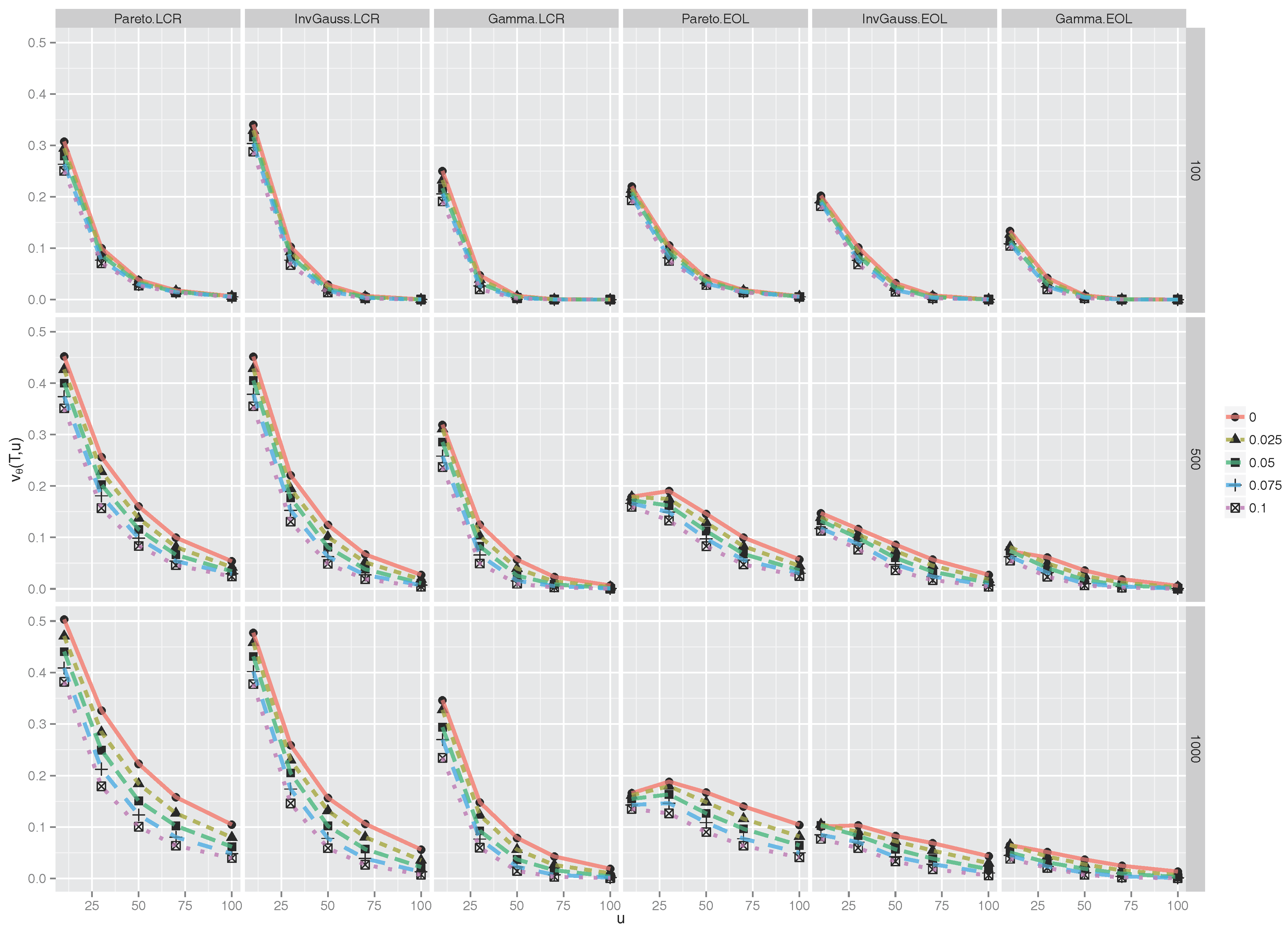
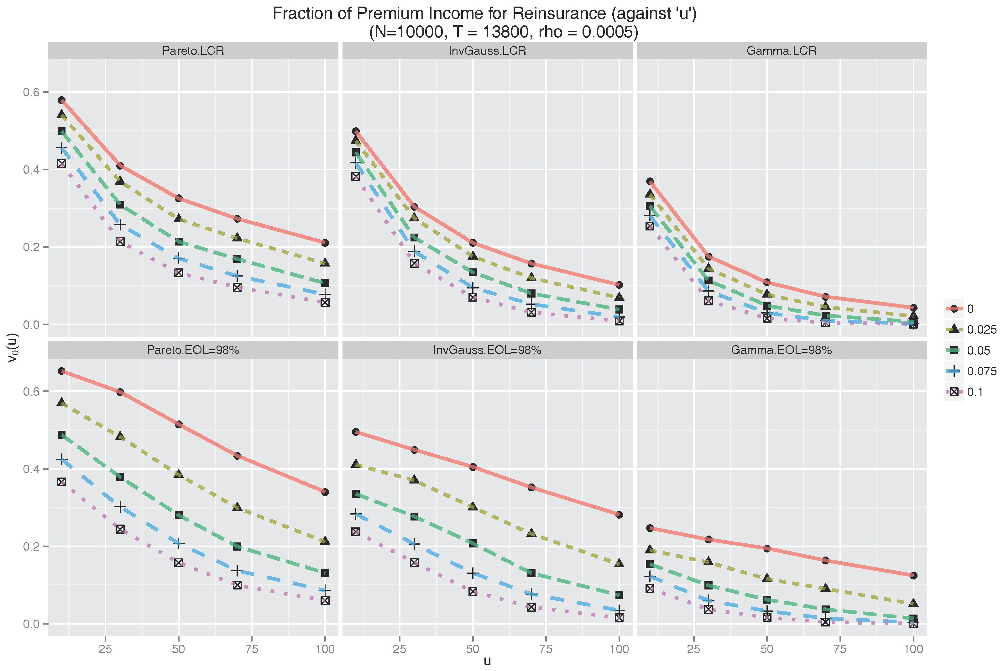
5.3. Proportion of Dividend Paid for Reinsurance

Figure 6 exhibits the graph of $v_{\theta }\left(u\right)$ (see (32)) for each of the LCR and EOL treaties under each of the three claims distributions. For the EOL treaty, L is taken as the 98th percentile of the claims distribution. This percentile was chosen after some experimentation to give similar values for $v_{\theta }\left(u\right)$ in the LCR and EOL cases.

In both the LCR and EOL frameworks, we observe from Figure 6 that $v_{\theta }\left(u\right)$ varies noticeably across u levels and distributions. As the reserve level increases from $u=10$ to $u=100$, the proportion of the dividend the company is willing to pay for reinsurance drops significantly, for each value of θ. The rate of decrease is larger for smaller values of u for LCR but rather uniform across u values for EOL. As the safety loading increases, the insurance company is only willing to apportion a smaller part of the dividend toward reinsurance.

It is interesting to note that $v_{\theta }\left(u\right)$ is bounded by $0.65$ in all settings, indicating that the cedant is unwilling to pay more than $65\%$ of the dividend to reinsurance despite the high risk of ruin in cases when θ is low and u is low (e.g., $\theta =0$ and $u=10$). In this high risk region, ruin, though being likely (certain when $\theta =0$), will, with sufficient frequency, occur far enough into the future that the dividend stream lost due to ruin is negligible. Hence the cedant finds it unneccesary to dedicate more than 65% of dividend to reinsurance.

Since we have adopted a “utility indifference” rationale in calculating the premium, the expected values of the company, with and without reinsurance, are forced to be equal. This can also be readily checked: from (21), (23) and (31), we have

$$V_u^{\ast }=\frac{d_{max}^{\ast }\left(u\right)}{\rho }\mathbf{P}({\overline{Y}}_{{\mathbf{e}}_{\rho }}^{\ast }\le u)=\frac{d}{\rho }\mathbf{P}({\overline{Y}}_{{\mathbf{e}}_{\rho }}\le u)=V_u.$$

5.4. Standard Deviation of Dividend Income

In this section we compare the two reinsurance treaties, and the case with no reinsurance, with respect to the standard deviation of the dividend income. This will provide insight into the stabilising effect, or otherwise, of the reinsurance, which is a primary concern of the cedant company.

To calculate the standard deviation of the dividend income, observe that

$$\mathit{\sigma }\left(I_u\right)=\frac{d}{\rho }\mathit{\sigma }(1-e^{-\rho {\tau }_u}),$$

while for the reinsured portfolio, by (26),

$$\begin{array}{cc}\hfill \mathit{\sigma }\left(I_u^{\ast }\right)& =\frac{d_{max}^{\ast }\left(u\right)}{\rho }\mathit{\sigma }(1-e^{-\rho {\tau }_u^{\prime }})\hfill \\ & =\frac{d}{\rho }\frac{1-\mathbf{E}(e^{-\rho {\tau }_u};{\tau }_u<\infty )}{1-\mathbf{E}(e^{-\rho {\tau }_u^{\prime }};{\tau }_u^{\prime }<\infty )}\mathit{\sigma }(1-e^{-\rho {\tau }_u^{\prime }})\hfill \\ & =\frac{1-\mathbf{E}(e^{-\rho {\tau }_u};{\tau }_u<\infty )}{\mathit{\sigma }(1-e^{-\rho {\tau }_u})}\frac{\mathit{\sigma }(1-e^{-\rho {\tau }_u^{\prime }})}{1-\mathbf{E}(e^{-\rho {\tau }_u^{\prime }};{\tau }_u^{\prime }<\infty )}\left(\frac{d}{\rho }\mathit{\sigma }(1-e^{-\rho {\tau }_u})\right)\hfill \\ & =\frac{c_u^{\ast }}{c_u}\mathit{\sigma }\left(I_u\right),\hfill \end{array}$$

(33)

where $c_u$ is the coefficient of variation of $1-e^{-\rho {\tau }_u}$ and $c_u^{\ast }$ is the coefficient of variation of $1-e^{-\rho {\tau }_u^{\prime }}$. Observe that the change in standard deviation is by a factor

$$s_{\theta }\left(u\right)=\frac{c_u^{\ast }}{c_u}$$

(34)

which, as for $v_{\theta }\left(u\right)$, depends on u and θ but not on d. Values of $s_{\theta }\left(u\right)$ are summarised in Figure 7, which shows a clear reduction in the standard deviation of the dividend income received, compared with the case of no reinsurance, across all distributions, reserve levels and safety loadings, for both LCR and EOL. The reduction is most significant under the Pareto claim distribution, lessening as the tail of the claim distribution becomes lighter.

As the safety loading θ increases, in almost all cases, the amount of variance reduction increases. However, looking across u levels, two clearly different trends emerge for LCR and EOL reinsurances. In the EOL setting, $s_{\theta }\left(u\right)$ decreases across all scenarios. In contrast, for LCR, $s_{\theta }\left(u\right)$ increases initially except for larger values θ in the Pareto case. Interestingly, small values of u exhibit the least variance reduction for EOL across all distributions, but, outside of the Pareto case, the most variance reduction for LCR, for the chosen parameters.

Overall, it may be adjudged that reinsurance has a non-trivial stabilising effect on the value of the company, particularly for heavier tailed claims distributions.

5.5. Dividend Adjustment and Reinsurance Premium, Finite Horizon

While it may be useful for planning and evaluation purposes to consider infinite horizon results, in practice a reinsurance treaty is not taken over an infinite time horizon, nor are dividends paid at a constant rate forever. Thus it is also prudent to value the company over a finite time horizon. In this case we should take into account both the value of the dividends paid, $V_{T,u}$, up to the expiration time T of the reinsurance treaty, and also the value of the (liquidated) portfolio, $F_{T,u}$, at time T. Thus, we replace (21) for the uninsured process with

$$V_{T,u}=\frac{d}{\rho }\left(1-\mathbf{E}{e}^{-\rho ({\tau }_u\wedge T)}\right),\mathrm{together}\mathrm{with}{F}_{T,u}=e^{-\rho T}\mathbf{E}(u-Y_T){\mathbf{1}}_{\{{\tau }_u>T\}}.$$

(35)

Similarly, for the reinsured process, (23) is replaced by

$$V_{T,u}^{\ast }=\frac{d^{\ast }}{\rho }\left(1-\mathbf{E}{e}^{-\rho ({\tau }_u^{\ast }\wedge T)}\right),\mathrm{together}\mathrm{with}{F}_{T,u}^{\ast }=e^{-\rho T}\mathbf{E}(u-Y_T^{\ast }){\mathbf{1}}_{\{{\tau }_u^{\ast }>T\}}.$$

(36)

By analogy with the infinite horizon case, we now wish to find the maximal reinsurance premium the cedant is willing to pay subject to ${\tau }_u^{\ast }\ge {\tau }_u$ a.s, $V_{T,u}^{\ast }\ge V_{T,u}$ and $F_{T,u}^{\ast }\ge F_{T,u}$4.

Applying the same logic as in Section 5.1, we find that $Y^{\ast }=Y^{\prime }$ is given by (24) and does not depend on $d^{\ast }$. Since $Y_t^{\prime }\le Y_t$ for all $t\in [0,T]$, the condition $F_{T,u}^{\ast }\ge F_{T,u}$ is automatically satisfied. Thus, arguing as before, the maximizing dividend rate $d_{max}^{\ast }(T,u)$ and the corresponding maximal reinsurance premium $r_{max}(T,u)$ (now both depending on T and u) are found by equating $V_{T,u}$ and $V_{T,u}^{\ast }$ in (35) and (36). Setting

$$v_{\theta }(T,u)=\frac{\mathbf{E}\left(e^{-\rho ({\tau }_u\wedge T)}-e^{-\rho ({\tau }_u^{\prime }\wedge T)}\right)}{1-\mathbf{E}{e}^{-\rho ({\tau }_u^{\prime }\wedge T)}}=1-\frac{\mathbf{P}({\overline{Y}}_{{\mathbf{e}}_{\rho }}\le u,{\mathbf{e}}_{\rho }\le T)}{\mathbf{P}({\overline{Y}}_{{\mathbf{e}}_{\rho }}^{\prime }\le u,{\mathbf{e}}_{\rho }\le T)},$$

(37)

(where the second equality in (37) follows from (A1) in the Appendix), we find that

$$d_{max}^{\ast }(T,u)=d\left[1-v_{\theta }(T,u)\right]\mathrm{and}{r}_{max}(T,u)=c^{\ast }-c+d{v}_{\theta }(T,u).$$

(38)

Observe that $0\le v_{\theta }(T,u)\le 1$, and, as in the infinite horizon case, $v_{\theta }(T,u)$ depends on u and θ but not on d. Thus, again, only a fixed proportion of the dividend is available to pay for reinsurance if the value of the firm is not to be reduced.

We simulated $v_{\theta }(T,u)$ with the parameters kept the same as in Table 1, Table 2 and Table 3 for LCR reinsurance and Table 4, Table 5 and Table 6 for EOL reinsurance. As mentioned previously, this is done to maintain comparability between the two reinsurance schemes. In particular L is not the 98-th percentile, as in the infinite horizon case, but is chosen according to (17). The results are summarized in Figure 8, which displays several interesting features.

For both types of reinsurance, the value of $v_{\theta }(T,u)$ is slightly higher for a Pareto claim distribution than for an Inverse Gaussian, which is greater again than for a Gamma claim distribution. This is consistent with the results for the ruin times in Table 1, Table 2, Table 3, Table 4, Table 5 and Table 6. It is notable that for $T=100$, $u=100$, regardless of θ and the claim distribution, the cedant is essentially unwilling to commit any of the dividend payment to reinsurance. Observe also that when the ruin probabilities under LCR and EOL are comparable in Table 1, Table 2, Table 3, Table 4, Table 5 and Table 6, the values of $v_{\theta }(T,u)$ are also comparable, whereas when the ruin probability under LCR is smaller than under EOL, for example when $u=10$ across all distributions, the cedant is able to contribute a larger portion of the dividend to reinsurance for LCR than EOL.

Considered as a function of u, $v_{\theta }(T,u)$ is decreasing and apparently convex in the case of the LCR treaty across all values of θ and T and all distributions, and this is also true for the EOL treaty in the $T=100$ case. For larger T, $v_{\theta }(T,u)$ is neither decreasing nor convex for EOL. Indeed for small u, $v_{\theta }(T,u)$ is seen to be increasing. As a function of T, for fixed θ and u, $v_{\theta }(T,u)$ is increasing for the LCR treaty. For the EOL treaty this is not the case since, for example, $v_{\theta }(T,u)$ is decreasing for $u=10$. Finally, for fixed T and u, the influence of the safety loading θ is much less pronounced than in Figure 6.

6. Related Literature and Discussion

In this section we mention some related results and propose possibly fruitful areas for future investigation.

6.1. Beveridge, Dickson and Wu Simulations

The work of [24] considers a model with a constant dividend barrier. Their insurance risk model incorporates a reinsurance arrangement h that applies to an individual claim, so that if the individual claim amount is x, the reinsurer pays $x-h\left(x\right)$, and the primary insurer retains $h\left(x\right)$, where $0\le h\left(x\right)\le x$. A dividend barrier, b, is specified such that when the surplus process, net of reinsurance, attains level b, dividends are paid out to shareholders at a specified rate $c^{\ast }$ until the next claim occurs. The modified surplus process remains at level b until the next claim occurs, then falls by the (net of reinsurance) amount of that claim. On any subsequent occasion that the net of reinsurance surplus process attains level b, dividends are again payable at rate $c^{\ast }$. Ruin occurs when the surplus process falls below zero, and no dividends are payable after the time of ruin. (See also [25,26,27].)

Under such a barrier scheme, the cedant’s ultimate ruin is certain, and the insurance operation is essentially being used to generate dividend income for the insurance company’s shareholders. The work of [24] investigates the effect of the reinsurance for two possible versions of the function h: proportional reinsurance, with $h\left(x\right)=ax$, where $0<a\le 1$, and excess of loss reinsurance, as we define it.

The emphasis of their study is different to ours, being mainly concerned with the value of net income to shareholders. They find for example that proportional reinsurance does not increase the expected present value of net income to shareholders, at least for the situations they consider, although “it is possible to increase the expected present value of net income to shareholders by effecting (EOL) reinsurance”. Other than this their results are mixed and not comparable with ours since in our setup ruin is not certain and we can investigate increases in ruin time with reinsurance and the other effects listed in Section 5.

6.2. Trimming More Values

The LCR scheme can be generalised by removing from the claims surplus process, not just the largest claim up to time t, but also the 2nd largest, 3rd largest, etc., up to a total of the r largest claims, $r=2,3,4,\dots$. In this connection [28] discuss two kinds of reinsurance systems in particular, using the nomenclatures ECOMOR and LCR. ECOMOR stands for excédent du coû moyen relatif. In this scheme, the reinsured amount is the sum of the differences between the r largest claims, and the r-th largest, $r=1,2,\dots$, up to a designated time. It was introduced into the actuarial literature by [29]. LCR in [28] is largest claims reinsurance as we define it, in which the reinsured amount is the sum of the r largest claims up to a designated time.

A considerable amount of work has been done on these and related methods; for background we refer to [30], who gives an overview of commonly used forms of reinsurance, and [28] for further literature. The [28] results 5 are concerned with limiting distributions of the reinsured amounts under the ECOMOR and LCR schemes, with subexponential, extremal class or regular variation assumptions on the tail of the claim distribution. They illustrate their results with simulations of the distributions.

Recall the discussion in Section 4.1, where we observed that the Inverse Gaussian case has several sizeable claims apart from the largest one. In order to achieve a similar level of efficiency for the reinsurance policy as in the Pareto case, the cedant can seek covers on the sum of the r largest claims. Then arises the question of an optimal choice of r, etc., which we do not go into here.

Some distributional identities for the r-trimmed version of a Lévy process have been studied in [31]. The continuity properties of various trimming functionals in cádlág space are investigated in [32]. Their formulae could be used to further analyse the first passage time (ruin time) and other path properties of r-trimmed processes.

6.3. The “Light-Medium-Heavy” Classification

It is important to stress that our division of claims distributions into “Light”, “Medium” and “Heavy”-tailed is not definitive, and the “lightness” of tails is not a uniquely defined concept. For example, if this were to be defined by whether the ratio of tails is asymptotically smaller for one than for the other, the “light-tailed” Gamma(2,1) distribution in (7) is judged “heavier” than the “medium”-tailed Inverse Gaussian in (11) for certain values of the parameters 6 a and b. Nevertheless, the classification is a useful way of specifying a range of tail behaviours on which to base simulation investigations.

The work of [33] gives a detailed analysis of the classical Norwegian Fire Claims data set, comparing a number of distributions for goodness of fit and using them to calculate value-at-risk and related measures. Of the six probability models considered some are heavy tailed, such as the GPD (generalised Pareto), others are lighter-tailed (the Weibull-Pareto). They argue “it is certainly tempting to conclude that simpler distributions, such as GPD and FT (folded-t) are preferred for the task of measuring tail risk” but “lead to substantially different risk evaluations”. This underlines the value of investigations like ours for understanding the behaviour of the risk process across a variety of tail regimens. The work of [33] further stress the need for formal statistical analysis for measuring and pricing tail risk.

In any case, as we discussed in Section 4.1, the behaviour of ruin probabilities and ruin times for finite u is not necessarily closely correlated with tail heaviness, however defined. These characteristics can be strongly influenced by the distribution of small and medium claim sizes. In this context we refer to discussions in [34,35] where asymptotic analyses of path properties of the process are given for convolution equivalent distributions, and related to the ruin prospects of the company.

On the other hand, of course, in any scenario, reinsurance in either of the ways we have defined it increases the lifetime of the company.

6.4. Lévy Insurance Risk Models

The LCR model can be extended in various directions. Insofar as our analysis is restricted to the classical compound Poisson risk process, it can be generalised to a broader class of processes, the “general Lévy insurance risk models”. See for example [7,8,9,10,36,37] , where these models and some subclasses of them are considered in this context.

7. Summary

We considered two types of reinsurance, EOL and LCR, and investigated the pros and cons of each by simulations. We took as outcomes the extent of increases in ruin times and decreases in ruin probabilities as a result of reinsurance. Using a dividend discount model, we also investigated the amount of the dividend available to pay for reinsurance and the consequent effect on the standard deviation of the company value.

We found in Section 4.2 that the EOL method performs markedly better than no reinsurance in terms of lower ruin probability and longer ruin times mainly when there are heavy tailed claims, whereas the LCR treaty shows consistent improvements over all three classes of claim distributions.

Regarding payment for reinsurance, we saw in Figure 6 and Figure 8 that for a Pareto claim distribution a greater proportion of the dividend is available to pay the reinsurance premium than for Inverse Gaussian, which is greater again than for a Gamma claim distribution. Over a finite time horizon, with equal expected aggregate claims, LCR is at least as effective as EOL in averting ruin (Table 1, Table 2, Table 3, Table 4, Table 5 and Table 6). When they are equally effective, the proportion of the dividend available to pay for reinsurance is comparable. When LCR is more effective, then the proportion is greater for LCR than for EOL (Figure 5). LCR and EOL both reduce risk considerably as compared with no reinsurance, in a variety of situations, as measured by the standard deviation of the dividend income.

multiple

References

1. K. Böcker. “and Klüppelberg, C. Multivariate models for operational risk.” Quant. Finance 10 (2010): 855–869. [Google Scholar] [CrossRef]
2. P. Embrechts, C. Klüppelberg, and T. Mikosch. Modelling Extremal Events for Insurance and Finance. Applications of Mathematics (New York); Berlin, Germany: Springer, 1997. [Google Scholar]
3. P. Embrechts, and G. Samorodnitsky. “Ruin problem and how fast stochastic processes mix.” Ann. Appl. Probab. 13 (2003): 1–36. [Google Scholar]
4. N. Doherty, and K. Smetters. “Moral hazard in reinsurance markets.” J. Risk Insur. 72 (2005): 375–391. [Google Scholar] [CrossRef]
5. Z. Yan. “Testing for moral hazard in reinsurance markets.” Manag. Finance 39 (2013): 696–713. [Google Scholar] [CrossRef]
6. S. Asmussen. Ruin Probabilities. Advanced Series on Statistical Science Applied Probability; Hackensack, NJ, USA: World Scientific Publishing Co., Inc., 2000, Volume 2. [Google Scholar]
7. R.A. Doney, C. Klüppelberg, and R.A. Maller. “Passage time and fluctuation calculations for subexponential Lévy processes.” Bernoulli 22 (2016): 1491–1519. [Google Scholar] [CrossRef]
8. C. Klüppelberg, A. Kyprianou, and R.A. Maller. “Ruin probabilities and overshoots for general Lévy insurance risk processes.” Ann. Appl. Probab. 14 (2004): 1766–1801. [Google Scholar] [CrossRef]
9. P.S. Griffin, R.A. Maller, and D. Roberts. “Finite time ruin probabilities for tempered stable insurance risk processes.” Insur. Math. Econom. 53 (2013): 478–489. [Google Scholar] [CrossRef]
10. P.S. Griffin, R.A. Maller, and K. van Schaik. “Asymptotic distributions of the overshoot and undershoots for the Lévy insurance risk process in the Cramér and convolution equivalent cases.” Insur. Math. Econom. 51 (2012): 382–392. [Google Scholar] [CrossRef]
11. R.J. Chhikara, and J.L. Folks. The Inverse Gaussian Distribution: Theory, Methodology, and Applications. New York, NY, USA: Marcel Dekker, 1989. [Google Scholar]
12. S. Asmussen, and K. Binswanger. “Simulation of ruin probabilities for subexponential claims.” Astin Bull. 27 (1997): 297–318. [Google Scholar] [CrossRef]
13. H.U. Gerber. An Introduction to Mathematical Risk Theory. Monograph No. 8; Philadelphia, PA, USA: University of Pennsylvania, 1979, p. 478. [Google Scholar]
14. H.U. Gerber, and S. Loisel. Why Ruin Theory Should Be of Interest for Insurance Practitioners and Risk Managers Nowadays. Bruxelles, Belgium: Actuarial and Financial Mathematics, 2012. [Google Scholar]
15. G. Benktander. “Largest claims reinsurance (LCR). A quick method to calculate LCR-risk rates from excess of loss risk rates.” Astin Bull. 10 (1978): 54–58. [Google Scholar] [CrossRef]
16. R.M. Berglund. “A note on the net premium for a generalized largest claims reinsurance cover.” Astin Bull. 28 (1998): 153–162. [Google Scholar] [CrossRef]
17. E. Kremer. “Rating of largest claims and ECOMOR reinsurance treaties for large portfolios.” Astin Bull. 13 (1982): 47–56. [Google Scholar] [CrossRef]
18. E. Kremer. “Distribution-free upper bounds on the premiums of the LCR and ECOMOR treaties.” Insur. Math. Econom. 2 (1983): 209–213. [Google Scholar] [CrossRef]
19. E. Kremer. “The asymptotic efficiency of largest claims reinsurance treaties.” Astin Bull. 20 (1990): 11–22. [Google Scholar] [CrossRef]
20. E. Kremer. “Largest claims reinsurance premiums under possible claims dependence.” Astin Bull. 28 (1998): 257–267. [Google Scholar] [CrossRef]
21. J. Grandell. Aspects of Risk Theory. Springer Series in Statistics; New York, NY, USA: Springer, 1991. [Google Scholar]
22. N. Wikstad. “Exemplification of ruin probabilities.” Astin Bull. 6 (1971): 147–152. [Google Scholar] [CrossRef]
23. A.J. Bradshaw, M. Bride, A.B. English, D.J. Hindley, and G.P.M. Maher. Reinsurance and Retentions—A London Market Actuaries’ Group Paper. Arlington, VA, USA: Casualty Actuarial Society, 1991, Volume I. [Google Scholar]
24. C.J. Beveridge, D.C.M. Dickson, and X. Wu. “Optimal dividends under reinsurance.” Bulletin de l’Association Suisse des Actuaires 2 (2008): 149–166. [Google Scholar]
25. B. De Finetti. “Su un’impostazion alternativa dell teoria collecttiva del rischio.” Trans. Internat. Congr. Actuar. 2 (1957): 433–443. [Google Scholar]
26. D.C.M. Dickson, and H.R. Waters. “Some optimal dividends problems.” Astin Bull. 34 (2004): 49–74. [Google Scholar] [CrossRef]
27. H.U. Gerber, and E.S.W. Shiu. “Optimal dividends: Analysis with Brownian motion.” N. Am. Actuar. J. 8 (2004): 1–20. [Google Scholar] [CrossRef]
28. S.A. Ladoucette, and J.L. Teugels. “Reinsurance of large claims.” J. Comput. Appl. Math. 186 (2006): 163–190. [Google Scholar] [CrossRef]
29. A. Thépaut. “Une nouvelle forme de réassurance: Le traité d’excédent du coût moyen relatif (ECOMOR).” Bull. Trim. Inst. Actu. Fr. 49 (1950): 273–343. [Google Scholar]
30. J.L. Teugels. Reinsurance Actuarial Aspects. EURANDOM Report 2003-006; Eindhoven, The Netherlands: Technical University of Eindhoven, 2003. [Google Scholar]
31. B. Buchmann, Y. Fan, and R.A. Maller. “Distributional representations and dominance of a Lévy process over its maximal jump processes.” Bernoulli 22 (2016): 2325–2371. [Google Scholar] [CrossRef]
32. B. Buchmann, Y. Fan, and R.A. Maller. “Functional Laws for Trimmed Lévy Processes.” Available online: https://arxiv.org/abs/1609.07206 (accessed on 21 November 2016).
33. V. Brazauskas, and A. Kleefeld. “Modeling Severity and Measuring Tail Risk of Norwegian Fire Claims.” N. Am. Actuar. J. 20 (2016): 1–16. [Google Scholar] [CrossRef]
34. P.S. Griffin. “Convolution equivalent Lévy processes and first passage times.” Ann. Appl. Probab. 23 (2013): 1506–1543. [Google Scholar] [CrossRef]
35. P.S. Griffin, and R.A. Maller. “Path decomposition of ruinous behaviour for a general Lévy insurance risk process.” Ann. Appl. Probab. 22 (2012): 1411–1449. [Google Scholar] [CrossRef]
36. J. Garrido, and M. Morales. “On The expected discounted penalty function for Lévy risk processes.” N. Am. Actuar. J. 10 (2006): 196–216. [Google Scholar] [CrossRef]
37. A. Kyprianou. Introductory Lectures on Fluctuations of Lévy Processes with Applications. Berlin, Germany: Springer, 2006. [Google Scholar]
38. D.C.M. Dickson, and G.E. Willmot. “The density of the time to ruin in the classical Poisson risk model.” Astin Bull. 35 (2005): 45–60. [Google Scholar] [CrossRef]
39. M. Elghribi, and E. Haouala. “Laplace transform of the time of ruin for a perturbed risk process driven by a subordinator.” IAENG Int. J. Appl. Math. 39 (2009): 221–230. [Google Scholar]
40. F.D.P. Lima, J.M.A. Garcia, and A.D. Egídio dos Reis. “Fourier/Laplace transforms and ruin probabilities.” Astin Bull. 32 (2002): 91–105. [Google Scholar] [CrossRef]
41. E.A. Percheskii, and B.A. Rogozin. “On the joint distribution of random variables associated with fluctuations of a process with independent increments.” Theory Probab. Appl. 14 (1969): 410–423. [Google Scholar] [CrossRef]
• 1.The LCR procedure can be made prospective by implementing it as a forward looking dynamic procedure in real time, from the cedant’s point of view. Designate as time zero the time at which the reinsurance is taken out. At this time, the cedant company’s assets amount to u > 0 , say. The first claim arriving after time 0 is referred to the reinsurer and not debited to the cedant. Subsequent claims smaller than the initial claim are paid by the cedant until a claim larger than the first (the previous largest) arrives. The difference between these two claims is referred to the reinsurer and not debited to the cedant. The process continues in this way so that at time t, the accumulated amount referred to the reinsurer equals the largest claim up till that time. This procedure has the same effect as referring the largest claim up till time t retrospectively to the reinsurer.
• 2.Indeed, from a theoretical perspective, very little appears to be known about the effects of trimming on an insurance risk process and the subsequent ruin quantities. A series of approximate premium calculations for LCR treaties has been made in the literature; see, for example, [15,16], and [17,18,19,20], and their references.
• 3.The work of [23] suggests that one common principle in choosing L is to keep it at “a level at which claims become very infrequent”.
• 4.There are other possibilities here, for example requiring V T , u + F T , u V T , u + F T , u , instead of V T , u V T , u and F T , u F T , u . We chose our formulation since it most clearly mirrors the infinite horizon problem. The interested reader may investigate other versions of the optimization problem.
• 5.The work of [28] allows a generalised version of the compound Poisson model where the N t in (1) is replaced by a mixed Poisson process. But their simulations are done with the compound Poisson.
• 6.But our particular choice of a = 2 and b = 1.5 makes the Inverse Gaussian heavier-tailed than the Gamma(2,1).
Figure 1. A schematic illustration of the largest claim reinsurance (LCR) reinsurance scheme with a Pareto(1,2) claim distribution. Black dots indicate claim amounts and red lines are the successive amounts liable for the reinsurance company.
Risks 05 00003 g001
Figure 2. Sample paths of the insurance risk processes without reinsurance (black line), with LCR reinsurance (red line), and with EOL reinsurance (green line), for a Pareto(1,2) claim distribution. The company’s initial reserve is u = 10 , the safety loading is θ = 0.1 , expected claim size is µ = 2, claim arrival rate is λ = 1 , and each time unit is 0.01 year = 3.65 days. For comparability between the two schemes, the retention level L for the EOL scheme is chosen so that the expected values of the LCR and EOL aggregate claims are equal at maturity time T = 5000 .
Risks 05 00003 g002
Figure 3. Sample paths of the insurance risk processes without reinsurance (black line), with LCR reinsurance (red line), and with excess of loss (EOL) reinsurance (green line), for a Gamma ( 2 , 1 ) claim distribution. The safety loading is θ = 0.1 , expected claim size is µ = 2, claim arrival rate is λ = 1 , and each time unit is 0.01 years. L for the EOL scheme is chosen so that the expected values of the LCR and EOL claim distributions are equal at maturity time T = 5000 .
Risks 05 00003 g003
Figure 4. Sample paths of the insurance risk processes without reinsurance (black line), with LCR reinsurance (red line), and with EOL reinsurance (green line), for an IG ( 2 , 1.5 ) claim distribution. The safety loading is θ = 0.1 , expected claim size is µ = 2, claim arrival rate is λ = 1 , and each time unit is 0.01 years. L for the EOL scheme is chosen so that the expected values of the LCR and EOL claim distributions are equal at maturity time T = 5000 .
Risks 05 00003 g004
Figure 5. Tails of the three claim distributions involved in our simulations.
Risks 05 00003 g005
Figure 6. v θ ( u ) (from (32)) is the proportion of the dividend available to pay for reinsurance without reducing the value of the firm. For Pareto, Inverse Gaussian and Gamma claim distributions, initial reserve levels u = 10 , 30, 50, 70, 100, time value of money ρ = 0.0005 , and safety loadings θ = 0 , 0.025, 0.05, 0.075, 0.1. Top panel: LCR; bottom panel, EOL with L taken as the 98th percentile of the claims distribution. Simulations are done with N = 10 , 000 sample paths.
Risks 05 00003 g006
Figure 7. s θ ( u ) (from (34), obtained by approximation at T = 13 , 800 ) is the ratio of the standard deviation of the dividend income obtained under reinsurance, to that without (infinite horizon case). For Pareto, Inverse Gaussian and Gamma claim distributions, initial reserve levels u = 10 , 30, 50, 70, 100, time value of money ρ = 0.0005 , and safety loadings θ = 0 , 0.025, 0.05, 0.075, 0.1. Top panel: LCR; bottom panel, EOL, with L taken as the 98th percentile of the claims distribution. Simulations are done with N = 10 , 000 sample paths.
Risks 05 00003 g007
Figure 8. v θ ( T , u ) (from (37)) is the proportion of the dividend available to pay for reinsurance without reduing the value of the firm. For LCR and EOL reinsurance policies, Pareto, Inverse Gaussian and Gamma claim distributions, initial reserve levels u = 10 , 30, 50, 70, 100, time value of money ρ = 0 . 0005 , and safety loadings θ = 0 , 0.025, 0.05, 0.075, 0.1. Top panel: T = 100 ; Middle panel: T = 500 ; Bottom panel: T = 1000 . Retention level L for EOL reinsurance is the solution to (17). For T = 100 , L ( T ) = 5.64 , 6.89, 4.49; for T = 500 , L ( T ) = 12.62 , 11.27, 6.10; for T = 1000 , L ( T ) = 17.84 , 13.39, 6.79 for Pareto, Inverse Guassian and Gamma distributions respectively. Simulations are done with N = 10 , 000 sample paths.
Risks 05 00003 g008