Minimum Protection in DC Funding Pension Plans and Margrabe Options

Abstract

The regulation on the Belgian occupational pension schemes has been recently changed. The new law allows for employers to choose between two different types of guarantees to offer to their affiliates. In this paper, we address the question arising naturally: which of the two guarantees is the best one? In order to answer that question, we set up a stochastic model and use financial pricing tools to compare the methods. More specifically, we link the pension liabilities to a portfolio of financial assets and compute the price of exchange options through the Margrabe formula.

1. Introduction

In most European countries, the sustainability of the pension system has become a major concern. The past few decades have therefore seen an evolution of the pension plan designs (as remarked e.g., by the European Commission, [1]). On one hand, more and more plans are financed through funding by pension funds or group/life insurance contracts (as opposed to plans financed through pay-as-you-go mechanisms). On the other hand, Defined Contribution (DC) schemes have tended to overtake Defined Benefit (DB) schemes. This new pension plan model (funding and DC) addresses—at least partially—the sustainability problem. However, it generates another issue, which is related to the adequacy of the benefits: in such a plan, the affiliates bear all of the financial risk.

To protect the affiliates and make these plans politically acceptable, many European countries have enacted legislations. Among various types of guarantees (presented e.g., in [2]), some of them impose on pension sponsors ensuring a minimum financial performance on plan contributions. The Swiss system is one of them, and an early and interesting example. Dating back to 1985, it imposes a minimal guaranteed rate that can be revised every other year by the Federal Council, which takes into account financial markets to do so. Accordingly, the rate was progressively lowered from $4\%$ (its value between 1985 and 2002) to its current level of $1.25\%$.

In 2003, Belgian authorities implemented the Law on Complementary Pension (LCP), obliging sponsors to guarantee a minimum rate of 3.25% on the employer’s contributions and of 3.75% on employees’ contributions. Since then, these values have proven to be unsustainable in the context of a decreasing interest rates market.

A reform act 1 has therefore been passed by the government (applicable since the beginning of 2016), that transforms the fixed minimum guaranteed rate into a variable rate, linked to the yield rate of the 10 year Belgian governmental bond. As it is fluctuating, one needs to indicate how the guarantee is applied to the previously paid contributions. Two different computation approaches are described in the new legal text, designated as the horizontal and vertical methods. In the case of newly created plans, sponsors are allowed to choose between them. On the contrary, in the case of already existing plans, the method that has to be used depends on the funding vehicle of the plan.

The existence of two computation methods raises the natural question of their comparison. In this paper, we address it by setting a stochastic framework for the interest rates and considering the evolution of the pension liability over the years. In order to compare the amounts obtained from one initial contribution using the horizontal and vertical methods, we embrace two distinct approaches. On one hand, we simply compute the expectations of the corresponding stochastic processes and determine which method leads to the best results. This approach can be associated with the affiliates’ point of view, as it estimates how much the affiliates will earn from the initial contribution.

On the other hand, we take the pension sponsor’s point of view and compute the price of both pension guarantees. The topic of pension guarantee pricing has been much studied in the literature (starting with the seminal papers of Pennacchi and Fischer [3,4] and going on after that with [5,6], among many others). More specifically, we follow an Asset and Liability Management-driven methodology (as done for example in [7,8,9]): we suppose that the sponsor has an asset investment portfolio in front of its pension liabilities, and we try to determine which method is preferable for him, taking into account its investment preferences. In order to do so, we consider options allowing for exchanging the asset portfolio for the horizontal (respectively vertical) liability and compute their prices: the best method is the one associated to the cheapest option. This methodology has already been used, for example in [10]. The pricing of these exchange options is achieved using the Margrabe formula (see [11]). More precisely, we use a generalization of this formula to a stochastic interest rates framework obtained (in the general case, where assets and rates are not independent) by Bernard and Cui [12] (see also [13]).

The paper is organized as follows: in Section 2, we present the details of the reform act, such as the definition of the guaranteed rate, and describe the horizontal and vertical computation methods. Then, we set up a stochastic framework and perform the first comparison of the two methods in Section 3. Section 4 is devoted to our second comparison approach, using option prices and the Margrabe formula. Finally, we comment on the results and conclude in Section 5.

2. Detailed Design of the Reform Act

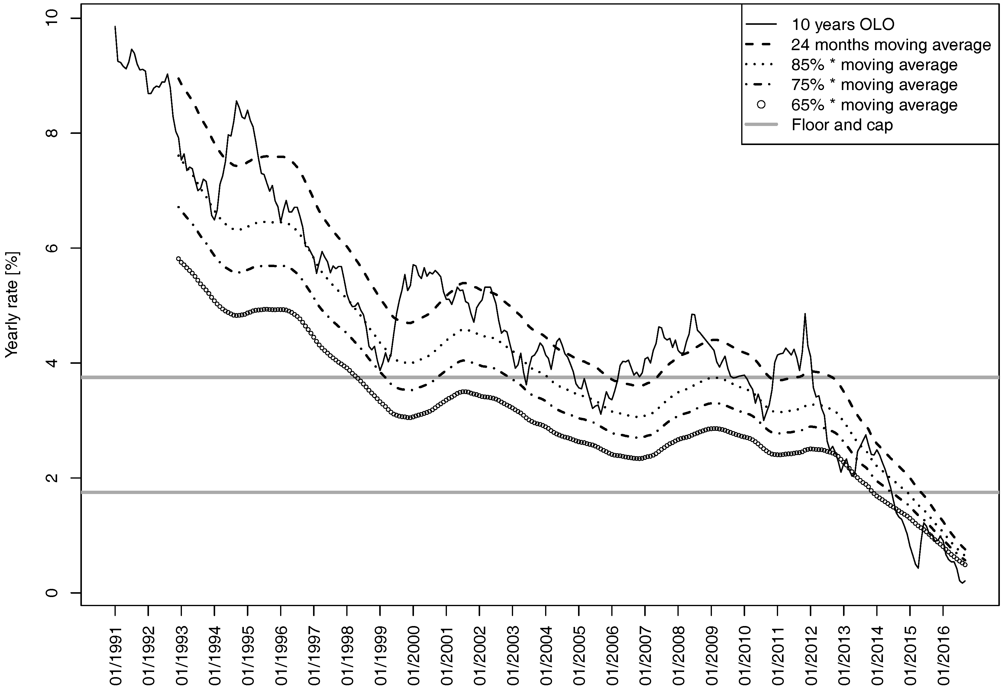
The new LCP links the guaranteed rate to a 24-month moving average of the 10-year OLO (i.e., Belgian governmental bond) yield rate . A cap and a floor is applied to this average, and the result is multiplied by a constant:

$$r_{\mathrm{guaranteed}}\left(t_0\right)=max\left(1.75\%;min\left(\pi \frac{1}{24}\sum _{t=0\mathrm{months}}^{23\mathrm{months}}{r}_{\mathrm{OLO}10}(t_0-t);3.75\%\right)\right).$$

The value of π is defined as $65\%$, but the law states that, under some circumstances (which are linked to the evolution of the maximum rate of long-term insurance contracts), the National Bank of Belgium can decide to raise this percentage to 75% in 2018 and to 85% in 2020. Figure 1 shows the evolution of these rates between January 1991 and September 2015.

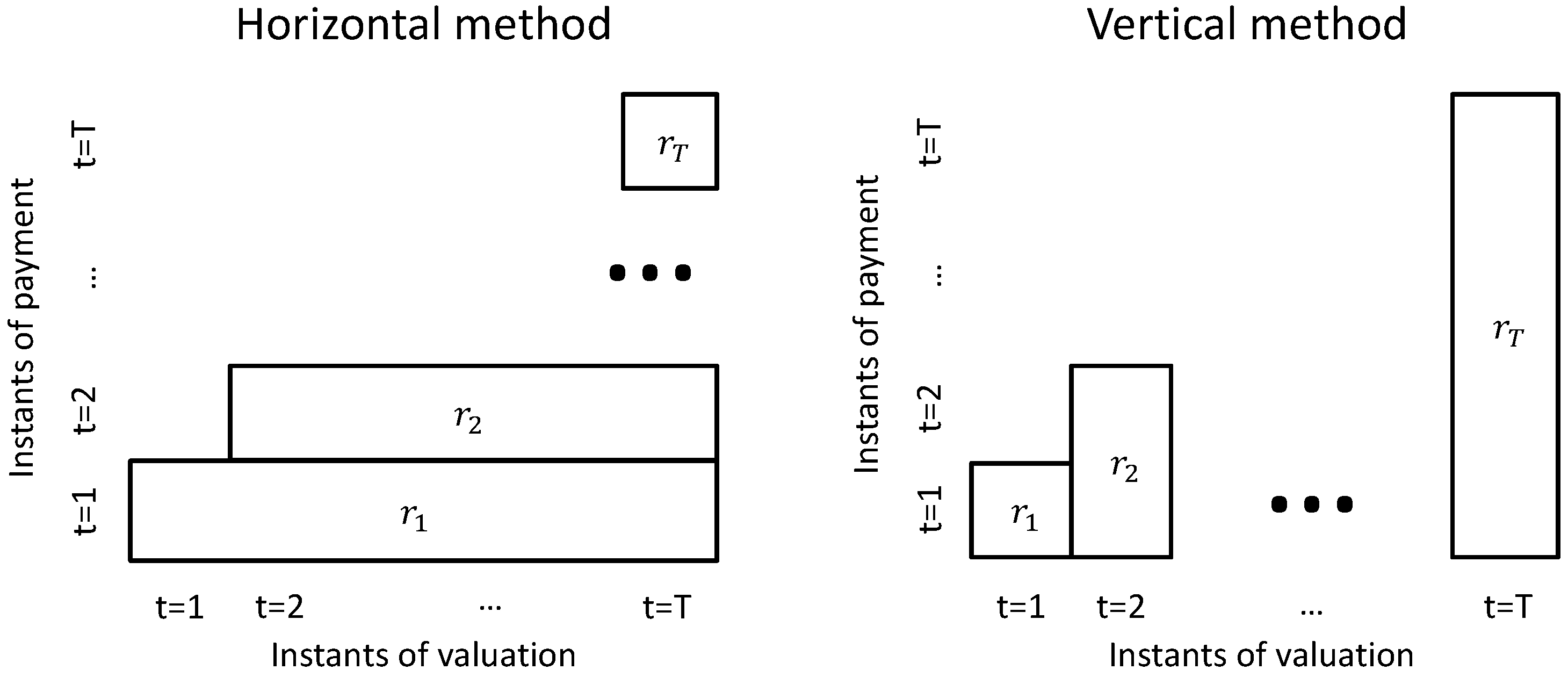
Let us now present the two computation methods, which are summarized in Figure 2. The vertical method is used when the vehicle of an existing pension scheme is a pension fund (or a pure unit linked product sold by an insurance company), or when the sponsor of a new pension scheme (i.e., created before 1 January 2015) chooses so. In this case, the guaranteed rate of year t is applied to the whole amount of cotisations already paid by the affiliated up to year t. The vertical liability is then similar to the one produced by a savings product where the contributions are deposited, whose interest rate is the guaranteed rate, susceptible to be different from year to year.

The horizontal method is used when the financing vehicle is a life insurance contract with interest rate guarantee or when the sponsor of a new pension scheme chooses so. Remark that, in this case, the guarantee level offered by the insurer can be different from the guarantee level that the sponsor must legally ensure to its affiliates. The guaranteed rate of year t is then applied to the new cotisations paid in year t, the cotisations already paid in years $t-1$ being accounted for with the guaranteed rate of year $t-1$, etc. The resulting horizontal liability is similar to the one produced by a standard life insurance product.

Let us first consider a very simple example to illustrate the two methods: assume that an affiliate successively pays two contributions of 1 Euro in 2016 and 2017, and retires in 2018. In

Table 1. Simple example illustrating how the horizontal and vertical methods are applied to the plan contributions.

	Scenario 1	Scenario 2
2016 guaranteed rate	$2.5\%$	$2.5\%$
2017 guaranteed rate	$3.5\%$	$2\%$
2018 liability (horizontal)	${1.025}^2+1.035=2.086$	${1.025}^2+1.02=2.071$
2018 liability (vertical)	$1.025·1.035+1.035=2.096$	$1.025·1.02+1.02=2.066$
Highest liability	vertical	horizontal

, we consider two scenarios for the evolution of the guaranteed interest rate.

Although very simple, this small toy example provides some intuition about the relation between the two computation methods and the market evolution. If the interest rates are increasing, the vertical method leads to a larger amount. If, on the contrary, the interest rates are decreasing, the horizontal liability is larger.

3. Direct Comparison

In this section, we set up a stochastic framework for the interest rates and use it to compare the level of the two guarantees in absolute terms.

3.1. Interest Rate Framework

We assume that the short rate $r_t$ is modelled with a Vasicek one-factor model, i.e., that in the risk-neutral world

$$\mathrm{d}{r}_t=k(\theta -r_t)\mathrm{d}t+\sigma \mathrm{d}{W}_t^r,$$

(1)

where $k>0$, $\sigma >0$ and θ are real constants and $W^r$ is a standard Brownian motion. It is well-known (see e.g., [14]) that the solution of this stochastic differential equation is

$$r_t=r_0{e}^{-kt}+\theta (1-e^{-kt})+\sigma {\int }_0^t{e}^{-k(t-s)}\mathrm{d}{W}_s^r,$$

(2)

and that the K-years zero-coupon bond yield is given by

$$r_t^K=\frac{C\left(K\right)+D\left(K\right)r_t}{K}=A\left(K\right)+B\left(K\right)r_t,$$

(3)

where

$$\begin{array}{cc}\hfill A\left(K\right)& =\frac{C\left(K\right)}{K},\hfill \\ \hfill B\left(K\right)& =\frac{D\left(K\right)}{K},\hfill \\ \hfill C\left(K\right)& =\left(\frac{{\sigma }^2}{2k^2}-\theta \right)\left(D\left(K\right)-K\right)+\frac{{\sigma }^2}{4k}{D}^2\left(K\right),\hfill \\ \hfill D\left(K\right)& =\frac{1}{k}\left(1-e^{-kK}\right).\hfill \end{array}$$

(4)

Note that, in the following, we will drop the K dependence and write $A=A\left(K\right)$ and $B=B\left(K\right)$ when the context is clear.

For simplicity reasons, and in order to obtain closed formula, we now make four assumptions. First, we replace the coupon-bearing reference bond instrument by a standard zero-coupon bond, i.e., we assume that the OLO bonds do not bear coupons. Second, we define the reference rate R as a three-year moving average of the market rate, instead of a 24-month moving average. This assumption strongly simplifies the notations but does not make the mathematical development easier. It also limits the smoothing effect of the moving average, but we think that it does not affect the hierarchy between the two methods. Third, we neglect the cap and floor applied to the market rate. It then follows from previous expressions that

$$R_t=\pi \frac{r_{t-2}^{10}+r_{t-1}^{10}+r_t^{10}}{3}.$$

Finally, we consider that the parameter π is constant, i.e., that the National Bank does not modify it during the considered period of time.

Note that we assume that the quantities $r_{-2}$, $r_{-1}$ and $r_0$ are known at $t=0$.

We consider a unique unitary payment made at time $t=0$ and look at the capital generated by this payment after T years (with $T\ge 4$).

3.2. Expression of the Liability

When the horizontal method is used, the expression of the liability is very simple:

$$L_T^h=e^{R_{0}T}=exp\left(\pi A\left(10\right)T+\frac{B\left(10\right)\pi T}{3}\left(r_{-2}+r_{-1}+r_0\right)\right),$$

which is a deterministic quantity.

When, on the contrary, the vertical method is preferred, the liability is given by

$$L_T^v=\prod _{t=0}^{T-1}{e}^{R_t}=exp\left(\sum _{t=0}^{T-1}{R}_t\right).$$

(5)

The following proposition gives the distribution of this liability.

Proposition 1.

Under the assumptions stated above, the vertical liability at time T is given by

$$\begin{array}{cc}\hfill L_T^v& =exp\{\pi AT+\pi B\left(\frac{1}{3}{r}_{-2}+\frac{2}{3}{r}_{-1}+(1+\mathrm{\Lambda }\left(1\right))r_0+\theta (T-2-\mathrm{\Lambda }\left(1\right))\right)\hfill \\ & +\pi B\sigma {\displaystyle \sum _{t=1}^{T-1}}\mathrm{\Lambda }\left(t\right){\int }_{t-1}^t{e}^{ks}d{W}_s^r\},\hfill \end{array}$$

(6)

where

$$\begin{array}{cc}\hfill A& =A\left(10\right)andB=B\left(10\right),\hfill \end{array}$$

$$\begin{array}{cc}\hfill \lambda \left(t\right)& =\left\{\begin{array}{cc}1\hfill & ift=1,2,\cdots ,T-3\hfill \\ \frac{2}{3}\hfill & ift=T-2\hfill \\ \frac{1}{3}\hfill & ift=T-1\hfill \end{array}\right.,\hfill \end{array}$$

(7)

$$\begin{array}{cc}\hfill \mathrm{\Lambda }\left(t\right)& ={\displaystyle \sum _{u=t}^{T-1}}\lambda \left(u\right)e^{-ku}.\hfill \end{array}$$

(8)

In particular, $L_T^v\sim \mathcal{LN}\left(m_v\left(T\right),s_v^2\left(T\right)\right)$ with

$$\begin{array}{cc}\hfill m_v\left(T\right)& =\pi AT+\pi B\left(\frac{1}{3}{r}_{-2}+\frac{2}{3}{r}_{-1}+(1+\mathrm{\Lambda }\left(1\right))r_0+\theta (T-2-\mathrm{\Lambda }\left(1\right))\right),\hfill \\ \hfill s_v^2\left(T\right)& =\frac{{\pi }^2{B}^2{\sigma }^2(1-e^{-2k})}{2k}{\displaystyle \sum _{t=1}^{T-1}}{\mathrm{\Lambda }}^2\left(t\right)e^{2kt}.\hfill \end{array}$$

The proof of this result is given in the Appendix A.

3.3. Comparison of the Expectations

Intuition, guided by the example given in Table 1, suggests that the hierarchy between the two methods depends on the evolution of the markets: if they are increasing (resp. decreasing), the vertical (resp. horizontal) method produces a larger amount. An analysis of the results obtained in the less trivial stochastic framework presented in the preceding section shows that they go in that direction.

Table 2. Parameters used in the computations of the direct comparison.

k	σ	${\mathit{r}}_{\mathbf{0}}$	${\mathit{r}}_{-\mathbf{1}}$	${\mathit{r}}_{-\mathbf{2}}$
$0.15$	$0.41\%$	$1.34\%$	$1.34\%$	$1.34\%$

gives the parameters that were used in the computations. Remark that the Vasicek parameters (namely, k, σ and $r_0$) have been calibrated using historical OLO yield curves from 1991 to 2015.

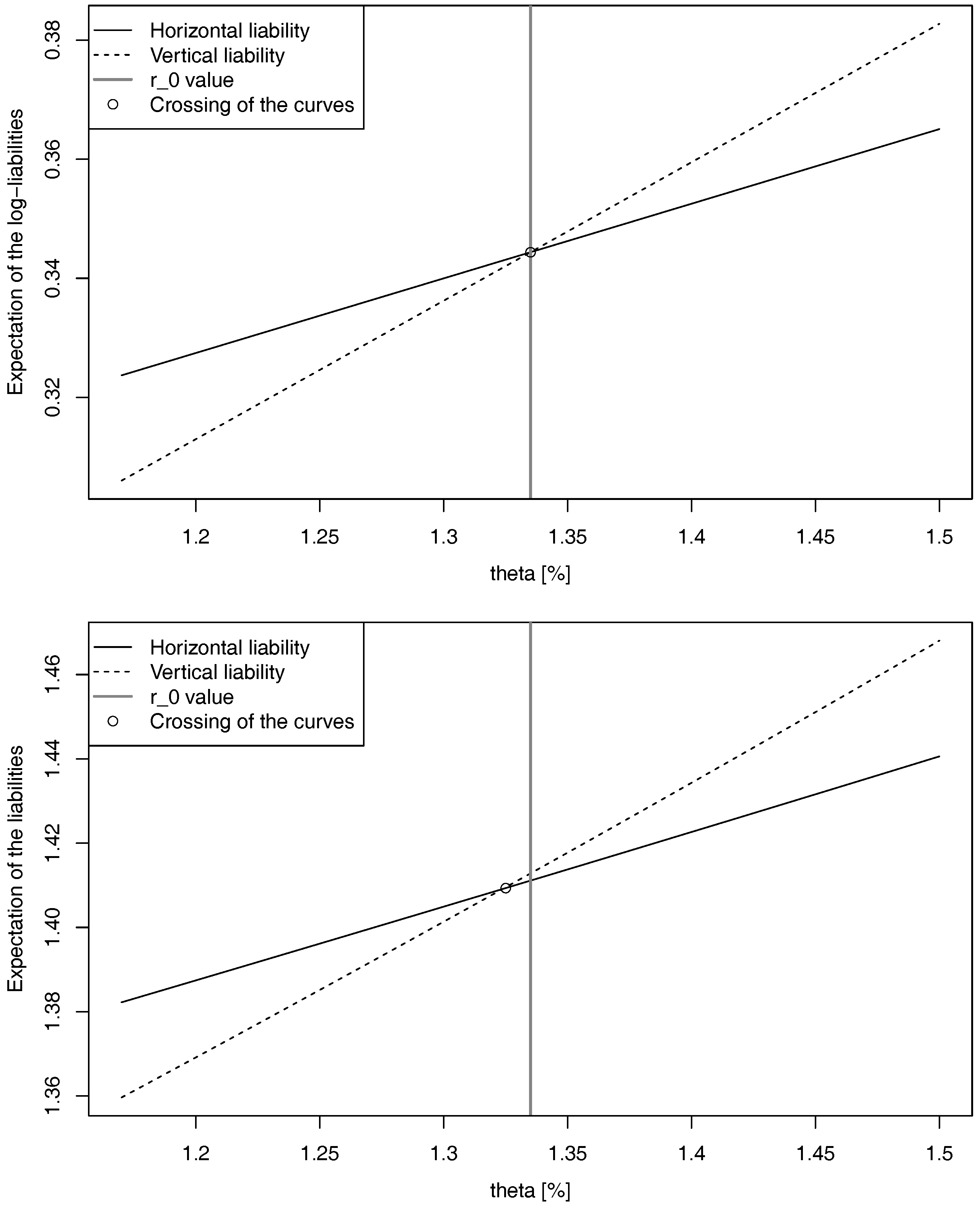
In Figure 3, we show the values of the four expectations:

$$\begin{array}{cc}\mathbb{E}\left[log\left(L_T^h\right)\right]=m_h\left(T\right);\hfill & \mathbb{E}\left[L_T^h\right]=exp\left(m_h\left(T\right)+\frac{s_h^2\left(T\right)}{2}\right)=exp\left(m_h\left(T\right)\right),\hfill \\ \mathbb{E}\left[log\left(L_T^v\right)\right]=m_v\left(T\right);\hfill & \mathbb{E}\left[L_T^v\right]=exp\left(m_v\left(T\right)+\frac{s_v^2\left(T\right)}{2}\right),\hfill \end{array}$$

when the parameter θ varies (the values of the other parameters are given in the appendix). We observe in the upper plot that, in accordance with the intuition, $r_0$ acts as a turning point:

$$\left\{\begin{array}{cc}{m}_h\left(T\right)>m_v\left(T\right)\hfill & \mathrm{if}\theta <r_0,\hfill \\ m_h\left(T\right)=m_v\left(T\right)\hfill & \mathrm{if}\theta =r_0,\hfill \\ m_h\left(T\right)<m_v\left(T\right)\hfill & \mathrm{if}\theta >r_0.\hfill \end{array}\right.$$

However, as is shown in the lower plot, another conclusion can be made for the expectations of the liabilities themselves, though the difference is not huge. There exists indeed another turning point, which is related but not equal to $r_0$. The reason for this phenomenon is the difference of volatility between the two liabilities ($0=s_h\left(T\right)<s_v\left(T\right)$).

4. ALM-Based Comparison

In this section, we compare the horizontal and vertical liabilities using an Asset and Liability Management approach. For this purpose, we assume that the organization offering the pension scheme to the affiliated invests the paid contributions in an investment portfolio. In order to compare the two methods, we compute the prices of two options giving the right to exchange the asset portfolio for the horizontal (resp. vertical) liability.

This is done using the well-known Margrabe formula (see [11]), which has been extended to a stochastic interest rates environment by [12]:

Proposition 2.

Let U and V be two non-dividend paying assets whose distributions are log-normal. If the short rate is a Brownian diffusion, the price of the European option whose pay-off at time T has the form ${(U_T-V_T)}_{+}$ is given by

$$M=U_0\mathsf{\Phi }\left(\frac{log\frac{U_0}{V_0}+\frac{1}{2}{\nu }^2\left(T\right)}{\nu \left(T\right)}\right)-V_0\mathsf{\Phi }\left(\frac{log\frac{U_0}{V_0}-\frac{1}{2}{\nu }^2\left(T\right)}{\nu \left(T\right)}\right),$$

(9)

with

$$\nu \left(T\right)=\sqrt{{\sigma }_U^2\left(T\right)+{\sigma }_V^2\left(T\right)-2c_{U,V}\left(T\right)},$$

where Φ is the cumulative distribution function of the standard normal, ${\sigma }_U\left(T\right)$ and ${\sigma }_V\left(T\right)$ are the standard deviations of $log\left(U_T\right)$ and $log\left(V_T\right)$, respectively, and $c_{U,V}\left(T\right)$ is the covariance between $log\left(U_T\right)$ and $log\left(V_T\right)$.

Note that, in the case of the horizontal liability (which is constant), the exchange option is identical to a standard put option. If the asset is log-normally distributed, the Margrabe formula thus reduces to the standard Black and Scholes formula (with stochastic interest rates).

4.1. Assets

We consider that the pension organizer has three investment opportunities: a bank deposit account, a rolling bond with fixed maturity and a stock. We first need to define the portfolio’s dynamics under the risk-neutral measure. The dynamics of the cash C is straightforwardly obtained from the short rate:

$$\mathrm{d}{C}_t=C_t{r}_t\mathrm{d}t.$$

The price of the rolling bond P with maturity K is related to the forward rate given in Equations (3) and (4):

$$P_t=exp\left(-C\left(K\right)-D\left(K\right)r_t\right),$$

so that, using the Itô formula, we easily obtain its dynamics:

$$\mathrm{d}{P}_t=P_t\left(r_t\mathrm{d}t-\sigma D\mathrm{d}{W}_t^r\right).$$

Finally, we assume that the stock S follows a geometric Brownian motion:

$$\mathrm{d}{S}_t=S_t\left(r_t\mathrm{d}t+\eta \rho \mathrm{d}{W}_t^r+\eta \sqrt{1-{\rho }^2}\mathrm{d}{W}_t^S\right),$$

where $\eta >0$ and $\rho \in [-1,1]$ are real parameters and $W^S$ is a standard Brownian motion that is independent from $W^r$.

We assume that the proportion of each asset in the portfolio A is kept constant over time, being $x\in [0,1]$ for stock, $y\in [0,1]$ for bond and $(1-x-y)\in [0,1]$ for cash. Obtaining an expression for the portfolio value is easy. First, we write its value as

$$A_t=N_t^C{C}_t+N_t^P{P}_t+N_t^S{S}_t,$$

where $N^C$, $N^P$ and $N^S$ are, respectively, the number of cash, rolling bond and stock units held at time t in the portfolio. Considering a self-financing portfolio, we obtain that

$$\mathrm{d}{A}_t=N_t^C\mathrm{d}{C}_t+N_t^P\mathrm{d}{P}_t+N_t^S\mathrm{d}{S}_t,$$

or, equivalently, that

$$\begin{array}{cc}\hfill N_t^C& =(1-x-y)\frac{A_t}{C_t},\hfill \\ \hfill N_t^P& =y\frac{A_t}{P_t},\hfill \\ \hfill N_t^S& =x\frac{A_t}{S_t}.\hfill \end{array}$$

The dynamics of A are therefore given by

$$\frac{\mathrm{d}{A}_t}{A_t}=r_t\mathrm{d}t+x\eta \sqrt{1-{\rho }^2}\mathrm{d}{W}_t^S+(x\eta \rho -y\sigma D)\mathrm{d}{W}_t^r.$$

The solution of the preceding equation can be easily obtained using the Itô formula:

$$\begin{array}{cc}\hfill A_T& =A_{0}exp\left({\int }_0^T{r}_s\mathrm{d}s-\frac{1}{2}(x^2{\eta }^2+y^2{\sigma }^2{D}^2-2\rho xy\eta \sigma D)T\right.\hfill \\ & \left.+x\eta \sqrt{1-{\rho }^2}{W}_T^S+(x\eta \rho -y\sigma D)W_T^r\right)\hfill \\ & =A_{0}exp\left(\theta T+\frac{r_0-\theta }{k}(1-e^{-kT})-\frac{1}{2}(x^2{\eta }^2+y^2{\sigma }^2{D}^2-2\rho xy\eta \sigma D)T\right.\hfill \\ & \left.+{\int }_0^T\left(\gamma -\frac{\sigma }{k}{e}^{-k(T-s)}\right)\mathrm{d}{W}_s^r+x\eta \sqrt{1-{\rho }^2}{W}_T^S\right),\hfill \end{array}$$

where

$$\gamma =\frac{\sigma }{k}+x\eta \rho -y\sigma D$$

so that $A_T\sim \mathcal{LN}\left(m_a\left(T\right),s_a^2\left(T\right)\right)$ with

$$\begin{array}{cc}\hfill s_a^2\left(T\right)& ={\int }_0^T{\left(\gamma -\frac{\sigma }{k}{e}^{-k(T-s)}\right)}^2\mathrm{d}s+x^2{\eta }^2(1-{\rho }^2)T\hfill \\ & =\frac{{\sigma }^2}{2k^3}(1-e^{-2kT})-2\frac{\sigma \gamma }{k^2}(1-e^{-kT})+\left({\gamma }^2+x^2{\eta }^2(1-{\rho }^2)\right)T.\hfill \end{array}$$

Remark that the asset allocation we consider here is constant over time. This is consistent with the investment habits of many Belgian pension funds and insurance companies. Some other pension funds around the world implement different strategies, e.g., following the affiliates’ risk preferences, and decreasing the volatility of the asset portfolios as the affiliates grow old. Generalizing the results, we obtain in the following sections that such a situation is not conceptually difficult, as we only have to replace the constants x and y by deterministic functions $x\left(t\right)$ and $y\left(t\right)$ in A’s dynamics. In particular, the asset random variable remains log-normally distributed.

4.2. Liabilities

As we have previously seen, the variables $A_T$ and $L_T^v$ are log-normally distributed under our asset and interest rate assumptions, and $L_T^h$ is constant. However, as $L^v$ and $L^h$ are not tradable assets, we have to define their fair values in order to apply the Margrabe formula (9):

$$U_t^h={\mathbb{E}}_Q\left[exp\left(-{\int }_t^T{r}_s\mathrm{d}s\right)L_T^h|{\mathcal{F}}_t\right]\mathrm{and}{U}_t^v={\mathbb{E}}_Q\left[exp\left(-{\int }_t^T{r}_s\mathrm{d}s\right)L_T^v|{\mathcal{F}}_t\right].$$

The processes $U^h$ and $U^v$ will successively play the role of U in Proposition 2, while the asset portfolio A will play the role of V. The payoffs of the considered options become then, respectively, ${(U_T^h-A_T)}^{+}$ and ${(U_T^v-A_T)}^{+}$. To apply Proposition 2 and compute their prices, we only have to compute three supplementary quantities: the initial fair values $U_0^h$ and $U_0^v$ and the covariance between the (logarithms of) $A_T$ and $L_T^v$.

To obtain $U_0^v$, we first integrate Equation (2) to obtain

$${\int }_0^T{r}_s\mathrm{d}s=\theta T+\frac{r_0-\theta }{k}(1-e^{-kT})+\frac{\sigma }{k}{\int }_0^T\left(1-e^{-k(T-s)}\right)\mathrm{d}{W}_s^r.$$

Putting this expression together with Formula (6) leads to

$$\begin{array}{cc}\hfill {\tilde{L}}_T^v& =exp\left(-{\int }_0^T{r}_s\mathrm{d}s\right)L_T^v\hfill \\ & =exp\{\pi AT+\pi B\left(\frac{1}{3}{r}_{-2}+\frac{2}{3}{r}_{-1}+(1+\mathrm{\Lambda }\left(1\right))r_0+\theta (T-2-\mathrm{\Lambda }\left(1\right))\right)\hfill \\ & -\theta T-\frac{r_0-\theta }{k}(1-e^{-kT})\hfill \\ & +{\displaystyle \sum _{t=1}^{T-1}}{\int }_{t-1}^t\left(\pi B\sigma \mathrm{\Lambda }\left(t\right)e^{ks}-\frac{\sigma }{k}(1-e^{-k(T-s)})\right)\mathrm{d}{W}_s^r\hfill \\ & -\frac{\sigma }{k}{\int }_{T-1}^T\left(1-e^{-k(T-s)}\right)\mathrm{d}{W}_s^r\},\hfill \end{array}$$

so that the discounted vertical liability ${\tilde{L}}_T^v\sim \mathcal{LN}\left({\tilde{m}}_v\left(T\right),{\tilde{s}}_v^2\left(T\right)\right)$ with

$$\begin{array}{cc}\hfill {\tilde{m}}_v\left(T\right)& =\pi AT+\pi B\left(\frac{1}{3}{r}_{-2}+\frac{2}{3}{r}_{-1}+(1+\mathrm{\Lambda }\left(1\right))r_0+\theta (T-2-\mathrm{\Lambda }\left(1\right))\right)-\theta T-\frac{r_0-\theta }{k}(1-e^{-kT}),\hfill \\ \hfill {\tilde{s}}_v^2\left(T\right)& =\frac{{\sigma }^2}{k^2}T+{\displaystyle \sum _{t=1}^{T-1}}\{\frac{{(\pi B\sigma \mathrm{\Lambda }\left(t\right)+\frac{\sigma }{k}{e}^{-kT})}^2}{2k}{e}^{2kt}\left(1-e^{-2k}\right)\hfill \\ & -\frac{2\sigma (\pi B\sigma \mathrm{\Lambda }\left(t\right)+\frac{\sigma }{k}{e}^{-kT})}{k^2}{e}^{kt}\left(1-e^{-k}\right)\}+\frac{{\sigma }^2}{k^3}\left(-\frac{3}{2}+2e^{-k}-\frac{1}{2}{e}^{-2k}\right).\hfill \end{array}$$

Now, $U_0^v$ is straightforwardly obtained, as it is the expectation of a log-normally distributed random variable

$$U_0^v=\mathbb{E}\left[\mathcal{LN}\left({\tilde{m}}_v\left(T\right),{\tilde{s}}_v^2\left(T\right)\right)\right]=exp\left({\tilde{m}}_v\left(T\right)+\frac{{\tilde{s}}_v^2\left(T\right)}{2}\right).$$

In addition, the initial value of the horizontal liability is easy to obtain, as

$$\begin{array}{cc}\hfill U_0^h& ={\mathbb{E}}_Q\left[exp\left(-{\int }_0^T{r}_s\mathrm{d}s\right)L_T^h\right]=L_T^h{\mathbb{E}}_Q\left[exp\left(-{\int }_0^T{r}_s\mathrm{d}s\right)\right]\hfill \\ & =L_T^{h}P(0,T)=L_T^{h}exp\left(-C\left(T\right)-D\left(T\right)r_0\right).\hfill \end{array}$$

Finally, we compute, using Proposition 1,

$$\begin{array}{cc}\hfill c_{v,a}\left(T\right)& =cov\left[log\left(A_T\right),log\left(L_T^v\right)\right]\hfill \\ & =\mathbb{E}[\left({\int }_0^T\left(\gamma -\frac{\sigma }{k}{e}^{-k(T-s)}\right)\mathrm{d}{W}_s^r+x\eta \sqrt{1-{\rho }^2}{W}_T^S\right)\hfill \\ & ·\left(\pi B\sigma {\displaystyle \sum _{t=1}^{T-1}}\mathrm{\Lambda }\left(t\right){\int }_{t-1}^t{e}^{ks}\mathrm{d}{W}_s^r\right)]\hfill \\ & =\pi B\sigma {\displaystyle \sum _{t=1}^{T-1}}\mathrm{\Lambda }\left(t\right){\int }_{t-1}^t\left(\gamma -\frac{\sigma }{k}{e}^{-k(T-s)}\right)e^{ks}\mathrm{d}s\hfill \\ & =\pi B\sigma {\displaystyle \sum _{t=1}^{T-1}}\mathrm{\Lambda }\left(t\right)\left(\frac{\gamma }{k}(e^{kt}-e^{k(t-1)})-\frac{\sigma }{2k^2}{e}^{-kT}(e^{2kt}-e^{2k(t-1)})\right).\hfill \end{array}$$

4.3. Comparison of Margrabe Option Prices

We are now able to compare the two liabilities using the ALM methodology explained supra. On one hand, the price of the option giving the right at time T to exchange the asset portfolio for the vertical liability is equal to

$$\begin{array}{cc}\hfill p_0^v=& exp\left({\tilde{m}}_v\left(T\right)+\frac{1}{2}{\tilde{s}}_v^2\left(T\right)\right)\mathsf{\Phi }\left(\frac{{\tilde{m}}_v\left(T\right)+\frac{1}{2}{\tilde{s}}_v^2\left(T\right)+\frac{1}{2}\left(s_v^2\left(T\right)+s_a^2\left(T\right)-2c_{v,a}\left(T\right)\right)}{\sqrt{s_v^2\left(T\right)+s_a^2\left(T\right)-2c_{v,a}\left(T\right)}}\right)\hfill \\ & -\mathsf{\Phi }\left(\frac{{\tilde{m}}_v\left(T\right)+\frac{1}{2}{\tilde{s}}_v^2\left(T\right)-\frac{1}{2}\left(s_v^2\left(T\right)+s_a^2\left(T\right)-2c_{v,a}\left(T\right)\right)}{\sqrt{s_v^2\left(T\right)+s_a^2\left(T\right)-2c_{v,a}\left(T\right)}}\right).\hfill \end{array}$$

On the other hand, the price of the option giving the right at time T to exchange the asset portfolio for the horizontal liability, which reduces to a standard put option on the asset portfolio with the strike being equal to the final value of the horizontal liability, is equal to

$$\begin{array}{cc}\hfill p_0^h& =-\mathsf{\Phi }\left(\frac{log\left(L_T^{h}P(0,T)\right)-\frac{1}{2}{s}_a^2\left(T\right)}{s_a\left(T\right)}\right)+L_T^{h}P(0,T)\mathsf{\Phi }\left(\frac{log\left(L_T^{h}P(0,T)\right)+\frac{1}{2}{s}_a^2\left(T\right)}{s_a\left(T\right)}\right).\hfill \end{array}$$

We can now compute these option prices for a set of various investment portfolios, using the parameters of Table 2 and

Table 3. Supplementary parameters used in the computations of the ALM comparison.

θ	K	η	μ
$1.34\%$	10	$25\%$	$5\%$

.

Table 4. Results of the ALM comparison for some example portfolios. The cheapest liability is the horizontal one when H is displayed, and the vertical one when V is displayed.

Description	Composition			Cheapest Liability
	x	y	z	$\mathit{\rho }=-1$	$\mathit{\rho }=-0.5$	$\mathit{\rho }=0$	$\mathit{\rho }=0.5$	$\mathit{\rho }=1$
Only stocks	100%	0%	0%	H	H	V	V	V
Only bonds	0%	100%	0%	H	H	H	H	H
Only cash	0%	0%	100%	V	V	V	V	V
Stocks and bonds	50%	50%	0%	H	H	V	V	V
Stocks and cash	50%	0%	50%	H	H	V	V	V
Bonds and cash	0%	50%	50%	V	V	V	V	V
Equal repartition	33%	33%	33%	H	H	V	V	V
Typical insurer portfolio	10%	80%	10%	H	H	V	V	V

gathers the results of the comparison. Among the example portfolios that we have considered, the “Typical insurer portfolio” is meant to mimic the investment habits of Belgian insurers. The prices of the two options are given in this case in

Table 5. Prices of the options giving the right to exchange the “Typical insurer” asset portfolio (as defined in Table 4) for the horizontal (resp. vertical) liability.

	$\mathit{\rho }=-1$	$\mathit{\rho }=-0.5$	$\mathit{\rho }=0$	$\mathit{\rho }=0.5$	$\mathit{\rho }=1$
$p_0^h$	$0.0044$	$0.0077$	$0.0112$	$0.0148$	$0.0183$
$p_0^v$	$0.0108$	$0.0099$	$0.0090$	$0.0082$	$0.0073$
$p_0^h-p_0^v$	$-0.0065$	$-0.0023$	$0.0022$	$0.0066$	$0.0111$

.

Let us first consider portfolios without any stock. In the case of the “only bonds” one, the horizontal liability is cheaper. This result is not really surprising, as this method looks like the way bonds produce money. On the contrary, in the case of the “only cash” portfolio, the vertical option price is smaller. Again, this conclusion is not unexpected because this method is similar to a savings product.

When stocks are included in the portfolio, the hierarchy between the methods depends on the correlation between stocks and rates. If $\rho >0$, the stock and the cash are similar in some sense. The vertical method is thus the cheapest one, as in the case of portfolios without stock. If, on the contrary, $\rho <0$, the asset portfolio is very different from cash, and the horizontal method is preferred.

The funding vehicle of the pension plan in question is therefore an important feature to consider when comparing the two computation methods. The nature of this institution has indeed a strong influence on its investment habits: insurers tend to invest a lot in bonds, while pension funds often prefer stocks.

5. Conclusions

The two comparison methodologies give different points of view of the two computation methods. The first one confirms what was trivially suggested by the intuition: the horizontal liability is larger than the vertical liability in the case of a decreasing rates market, and vice versa. The second methodology yields more interesting conclusions, as it connects the hierarchy between the two methods to the investment profile of the institution granting the guarantee. We have seen that two methods represent two different philosophies: the horizontal one is closer to the insurers’ asset management habits, while the vertical one is closer to pension funds’ investment preferences. For this reason, the reform act will possibly have consequences regarding the investment strategies of the Belgian pensions plans’ funding vehicles.

We have chosen to consider a valuation framework in order to be consistent with the IAS philosophy, and thus with the funding vehicles’ interests. It should, however, be noted that other methodologies would make sense. For example, it is possible to compute, instead of exchange option prices, risk measures (such as VaR or TVaR) applied to the gap between the asset portfolio value and the liability value.

Political circumstances have led Belgian authorities to let the choice for new pensions schemes, but, as the results generated by the two methods are different, a whole set of legal questions arise (out of scope here). Among them, we can mention discrimination problems (possible arbitrage by the sponsor, see e.g., [15,16,17]).

Our work leaves some questions open for further research, mainly in two directions. On one hand, we could consider the exact definition of the guaranteed rate, i.e., take into account the cap and the floor as defined in the legal text. In order to compute options prices similar to the ones that we have obtained with closed formulas, it would then be necessary to use numerical methods. On the other hand, we could consider more complex models for the interest rate and the stock price, including a more complete dependence structure between the two risk factors.