State Space Models and the Kalman-Filter in Stochastic Claims Reserving: Forecasting, Filtering and Smoothing

Abstract

This paper gives a detailed overview of the current state of research in relation to the use of state space models and the Kalman-filter in the field of stochastic claims reserving. Most of these state space representations are matrix-based, which complicates their applications. Therefore, to facilitate the implementation of state space models in practice, we present a scalar state space model for cumulative payments, which is an extension of the well-known chain ladder (CL) method. The presented model is distribution-free, forms a basis for determining the entire unobservable lower and upper run-off triangles and can easily be applied in practice using the Kalman-filter for prediction, filtering and smoothing of cumulative payments. In addition, the model provides an easy way to find outliers in the data and to determine outlier effects. Finally, an empirical comparison of the scalar state space model, promising prior state space models and some popular stochastic claims reserving methods is performed.

1. Introduction

At the end of each fiscal year, non-life insurance companies face the situation that the earned premiums are known, but not the outstanding loss liabilities. Consequently, one of the main tasks for actuaries in non-life insurance is to quantify accurately the outstanding loss liabilities. The outstanding claims reserves are often a large share of the liability side of the balance sheet, so it is very important for every non-life insurer to handle claims reserving adequately. It is not surprising, therefore, that over the past 40 years, numerous reserving methods have been developed, particularly since the early 1990s. These methods are based on various models (see Wüthrich and Merz (2008)), but rarely on time series models. This is surprising, especially in light of the fact that the claims process is a stochastic process, and claims data, as a sequence of discrete time data, represent time series.

In this paper, methods of claims reserving are considered, which are based on time series models, particularly on state space models. A state space model consists of a state equation describing the dynamics of the system and an observation equation establishing a link between the unobservable states of the system and the observations. Compared to other models, state space models have the advantage that the temporal dynamics of a system can often be detected more accurately. In addition, state space representations can be used flexibly to model univariate and multivariate, stationary and non-stationary time series or in cases of structural changes, interventions, missing data or other data irregularities. A consideration of state space models leads directly to the application of the Kalman-filter algorithms for parameter estimation, forecasting, filtering and smoothing. The Kalman-filter is generally distribution-free and provides the best linear predictors in the sense of minimizing the mean squared error (see Kalman (1960)).

There are currently 16 research papers in stochastic claims reserving on the topic of state space models and the Kalman-filter. Most of these state space representations are based on a calendar year approach, i.e., all available observations of one calendar year are stacked into one observation vector. The matrix-based approach of these models and the resulting Kalman recursions can complicate their applications. Therefore, to facilitate the implementation of state space models in practice, a new scalar approach is introduced in this paper. The resulting distribution-free scalar state space model for cumulative payments can be considered as an extension of the chain ladder (CL) method under the assumption that the observations in the upper triangle are based on unobservable states.

According to this content, the paper is structured as follows. Section 2 gives a brief overview of claims development triangles and the CL method. In Section 3, we present the previous papers in stochastic claims reserving on the topic of state space models, their contentual similarities and selected modeling approaches. Section 4 introduces the scalar state space model and gives derivations of the formulas for claims reserves and the mean squared error of prediction (MSEP). An empirical comparison of the scalar state space model and promising state space models, as well as popular stochastic claims reserving methods is given in Section 5. Finally, Section 6 provides concluding remarks.

2. Development Triangles and the CL Method

Statistical analysis of claims payments data is usually done by using claims development triangles. In this paper, we denote accident years by $i=0,\dots ,I$, development years by $j=0,\dots ,J$ and calendar years by $t=i+j$. We assume further that all claims are settled after the J-th development year. Cumulative payments in accident year i after j development years are denoted by $C_{i,j}$, and incremental payments in the j-th development year are denoted by $X_{i,j}$, respectively. An exemplary claims development triangle (see

Table 1. Cumulative payments in the claims development triangle of Taylor and Ashe (1983).

Accident	Development Year j
Year i	0	1	2	3	4	5	6	7	8	9
0	357848	1124788	1735330	2218270	2745596	3319994	3466336	3606286	3833515	3901463
1	352118	1236139	2170033	3353322	3799067	4120063	4647867	4914039	5339085
2	290507	1292306	2218525	3235179	3985995	4132918	4628910	4909315
3	310608	1418858	2195047	3757447	4029929	4381982	4588268
4	443160	1136350	2128333	2897821	3402672	3873311
5	396132	1333217	2180715	2985752	3691712
6	440832	1288463	2419861	3483130
7	359480	1421128	2864498
8	376686	1363294
9	344014

) is the dataset of Taylor and Ashe (1983), which includes data from the motor bodily injury class of business in one Australian state (1972–1981, quoted in Australian Dollars). Due to its popularity in claims reserving literature, the dataset of Taylor and Ashe (1983) acts like a kind of benchmark development triangle for claims reserving methods.

The CL method is probably the most popular loss reserving technique, and there are several stochastic models that could be used as a basis for the application of the CL method. In this paper, we introduce briefly the distribution-free CL model of Mack (1993).

Model Assumptions 1

(Distribution-free CL model of Mack (1993)).

⊳

Cumulative payments $C_{i,j}$ of different accident years i are stochastically independent.

⊳

There exist factors $f_0,\dots ,f_{J-1}>0$ and variance parameters ${\sigma }_0^2,\dots ,{\sigma }_{J-1}^2>0$, such that for all $i=0,\dots ,I$ and all $j=0,\dots ,J-1$, we have:

$$\begin{array}{cc}\hfill \mathbb{E}\left[C_{i,j+1}\right|C_{i,0},\dots ,C_{i,j}]=\mathbb{E}\left[C_{i,j+1}\right|C_{i,j}]& =f_j{C}_{i,j}\hfill \\ \hfill \mathrm{Var}\left(C_{i,j+1}\right|C_{i,0},\dots ,C_{i,j})=\mathrm{Var}\left(C_{i,j+1}\right|C_{i,j})& ={\sigma }_j^2{C}_{i,j}\hfill \end{array}$$

(1)

⊲

The development factors and variance parameters are then estimated using the (unconditionally) unbiased estimators:

$$\begin{array}{c}\hfill {\widehat{f}}_j=\frac{{\sum }_{i=0}^{I-j-1}{C}_{i,j+1}}{{\sum }_{i=0}^{I-j-1}{C}_{i,j}}\end{array}$$

(2)

and:

$$\begin{array}{c}\hfill {\widehat{\sigma }}_j^2=\frac{1}{I-j-1}\sum _{i=0}^{I-j-1}{C}_{i,j}{\left(\frac{C_{i,j+1}}{C_{i,j}}-{\widehat{f}}_j\right)}^2\end{array}$$

(3)

for $f_j$ and ${\sigma }_j^2$, respectively (for more details, see Mack (1993)).

3. Prior Applications in Stochastic Claims Reserving

This section presents the previous papers in claims reserving literature on the topic of state space models and the Kalman-filter, their relationships and selected modeling approaches of claims development data, as well as their state space representations.

3.1. Chronology and Categorization of the Papers

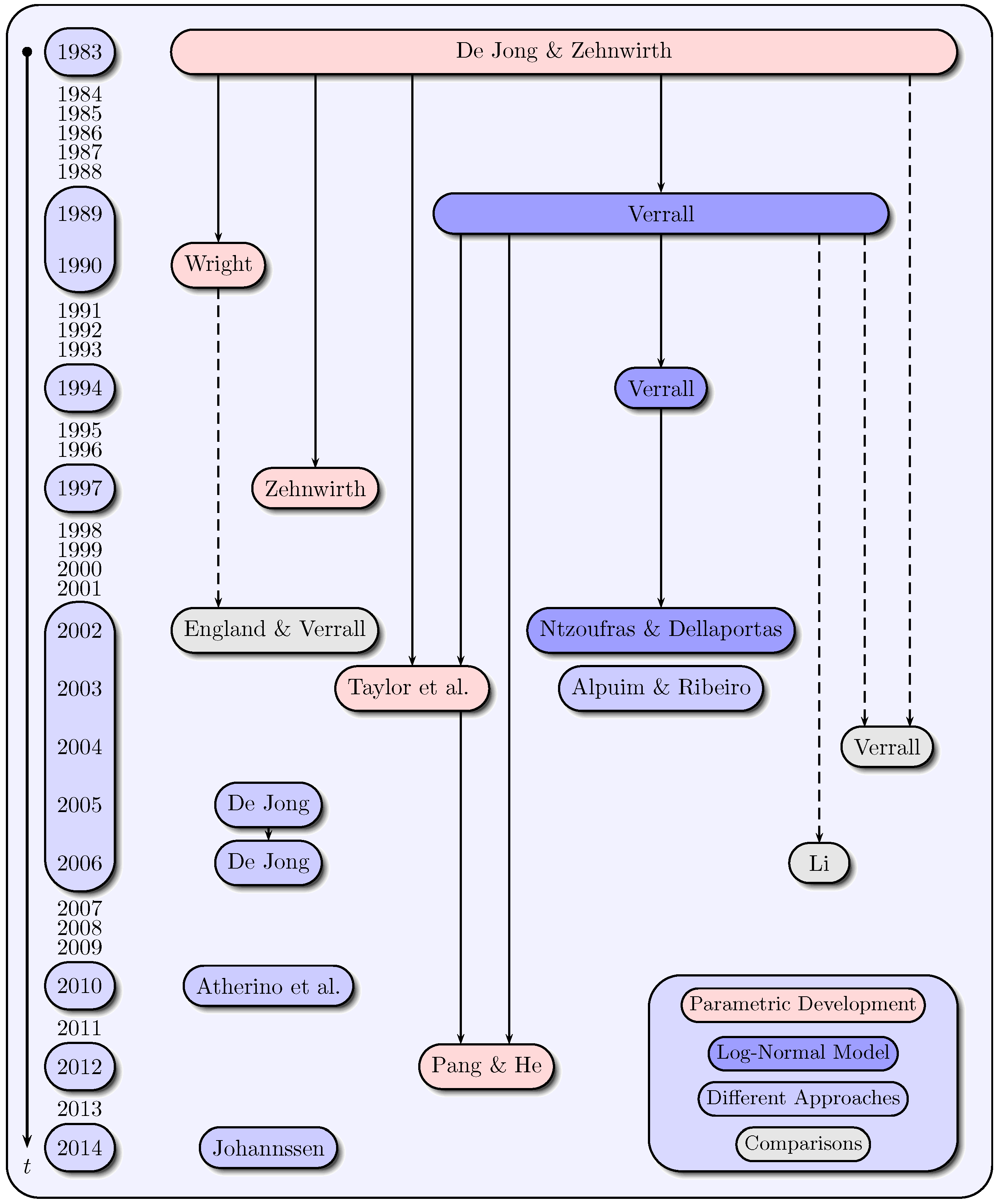
There are 16 papers in the claims reserving literature that are based on state space models and the Kalman-filter. Figure 1 displays these papers in chronological order and classifies them into four categories considering their substantial contentual similarities. The formulated categories “parametric development”, “log-normal model”, “different approaches” and “comparisons” need not be taken as mutually exclusive. Instead, the choice of the appropriate category is made considering the main approach used in the respective paper. In the papers of the first category a parametric development of claims data over the development years is assumed. The papers of the second category are based on the log-normal model for incremental payments, while in the third category, different approaches are aggregated. The fourth category unites comparisons of various reserving methods. The solid arrows in Figure 1 represent the contentual similarities among the papers in modeling approaches. The dashed arrows indicate, however, that the respective models are included in the papers of the fourth category that compares various models.

3.2. Modeling of Claims Development Data

In the first category, the authors De Jong and Zehnwirth (1983), Wright (1990), Zehnwirth (1997), Taylor et al. (2003) and Pang and He (2012) mainly use variations on the Hoerl curve to model the claims data over the development years. The general exponential-logarithmic Hoerl curve is given as ${\beta }_j=\exp (\kappa j+\delta \log j)$ with development year parameter ${\beta }_j$ for all $j=0,\dots ,J$ and $\kappa ,\delta \in \mathbb{R}$. An advantage of treating development time j as a continuous covariate is that extrapolation is possible beyond the range of development times observed (see Frees (2010) and Kaas et al. (2009)). As a variation, De Jong and Zehnwirth (1983), for example, define incremental payments $X_{i,j}$ as:

$$\begin{array}{c}\hfill X_{i,j}={\alpha }_i(j+1)e^{-j}+w_{i,j}\end{array}$$

(4)

with accident year parameter ${\alpha }_i$ and $w_{i,j}\sim WN\left(0;{\sigma }_w^2\right)$ for all $i=0,\dots ,I$ and $j=0,\dots ,J$. To allow a dynamic recursive estimation of the accident year parameters and to avoid over-parametrization, they assume the accident year parameters evolve in the way ${\alpha }_{i+1}={\alpha }_i+v_i$ with ${\alpha }_0=0$ and $v_i\sim WN\left(0;{\sigma }_v^2\right)$. The modeling (4) leads to the general shape of incremental payments curve over the development years, i.e., the incremental payments are supposed to rise very fast in early development years and to decrease exponentially over the following development years.

The models in the papers of the first category are mostly distribution-free in contrast to the papers of the second category (Verrall (1989,1994), Ntzoufras and Dellaportas (2002)), in which incremental payments are assumed to follow a log-normal distribution. The logarithmic incremental payments are specified by the log-normal model:

$$\begin{array}{c}\hfill Y_{i,j}=\log \left(X_{i,j}\right)=\mu +{\alpha }_i+{\beta }_j+w_{i,j}\end{array}$$

(5)

with $X_{i,j}>0$, mean $\mu$, accident year parameter ${\alpha }_i$, development year parameter ${\beta }_j$ and the Gaussian white noise process $w_{i,j}\sim WN\left(0;{\sigma }_w^2\right)$ for all $i=0,\dots ,I$ and $j=0,\dots ,J$. The accident and development year parameters are further assumed to evolve as follows for the same reasons as in De Jong and Zehnwirth (1983):

$$\begin{array}{c}\hfill \begin{array}{c}\hfill {\alpha }_{i+1}={\alpha }_i+v_i^{\left(\alpha \right)}\\ \hfill {\beta }_{j+1}={\beta }_j+v_j^{\left(\beta \right)}\end{array}\end{array}$$

(6)

with ${\alpha }_0={\beta }_0=0$ and white noise processes $v_i^{\left(\alpha \right)}$ and $v_j^{\left(\beta \right)}$ for all $i=0,\dots ,I$ and $j=0,\dots ,J$. Model (5) was also named as the “linear CL model” by Verrall (1989,1994), since it is very similar to an additive representation of the CL method (see also Kremer (1982)). In addition to the basic model (5), which is used by Verrall (1989) and Li (2006), Verrall (1994) and Ntzoufras and Dellaportas (2002) extend the basic model by integrating varying run-off evolutions.

As a first example of the third category, Atherino et al. (2010) consider a different data ordering of non-cumulative run-off triangles, in which the stacked rows of a triangle form a univariate time series $y_t$ with several runs of missing data. They choose a structural model for the incremental payments with a local level component ${\nu }_t$, a stochastic periodic component ${\eta }_t$ and a regression term ${\mathbf{h}}_t^T\mathbf{u}$,

$$\begin{array}{cc}\hfill y_t& ={\nu }_t+{\eta }_t+{\mathbf{h}}_t^T\mathbf{u}+w_t\hfill \end{array}$$

(7)

$$\begin{array}{cc}\hfill {\nu }_{t+1}& ={\nu }_t+v_t^{\left(\nu \right)}\hfill \end{array}$$

(8)

$$\begin{array}{cc}\hfill {\eta }_{t+1}& =-\sum _{d=1}^{J-1}{\eta }_{t+1-d}+v_t^{\left(\eta \right)}(t=J-1,J,\dots )\hfill \end{array}$$

(9)

with the Gaussian white noise processes $w_t$, $v_t^{\left(\nu \right)}$, $v_t^{\left(\eta \right)}$. This model and its components are motivated by the claims process behavior: The level component shall respond for the average value of claims along each accident year, while the periodic component is supposed to capture the development year effect. The regression term is mainly motivated by the need for intervention effects due to the presence of outliers.

Another example of the third category to model the claims data can be found in Alpuim and Ribeiro (2003). They assume that the incremental payments $X_{i,j}$ for the i-th accident year ($i=0,\dots ,I$) in the j-th development year ($j=1,\dots ,J$) depend on the payments $X_{i,0}$ of the respective accident year,

$$\begin{array}{c}\hfill X_{i,j}={\lambda }_{i,j}{X}_{i,0}+w_{i,j}\end{array}$$

(10)

with $w_{i,j}\sim WN\left(0;{\sigma }_w^2\right)$. That is, the total amount of claims incurred in year i and paid j years later is proportional to the claims incurred and paid in accident year i. This proportion varies randomly with development and accident year, so that they assume for the proportion parameter ${\lambda }_{i,j}$ a first order autoregressive process:

$$\begin{array}{c}\hfill {\lambda }_{i,j}={\mu }_j+{\varphi }_j({\lambda }_{i-1,j}-{\mu }_j)+v_{i,j}\end{array}$$

(11)

with mean ${\mu }_j$ and $v_{i,j}\sim WN\left(0;{\sigma }_v^2\right)$. Moreover, the $X_{i,j}$ of different development years $j=1,\dots ,J$ are stochastically independent.

Since the fourth category (England and Verrall (2002), Verrall (2004), Li (2006)) provides comparisons of various methods, there is only a recapitulation of existing approaches in the remaining papers.

All of these modeling approaches can be converted into a state space representation, and then, the Kalman-filter can be used for prediction, filtering and smoothing of the claims development data.

3.3. Modeling Approaches of State Space Representations

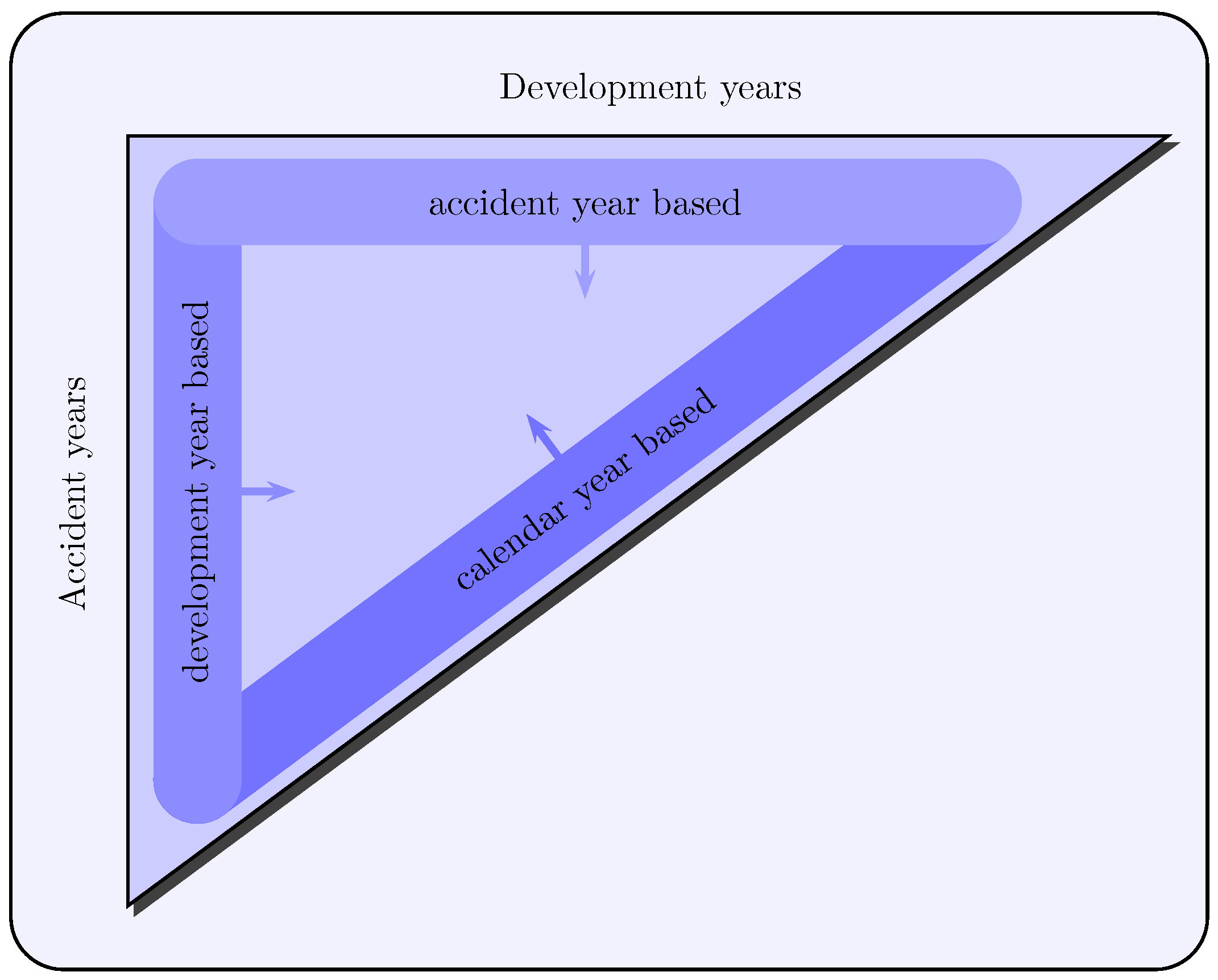
Most of state space representations in the introduced papers are based on the calendar year approach, which provides the claims data of each calendar year to be stacked into separate observation vectors of the respective calendar years. In addition to this approach, there are further differing approaches considering an accident year- or a development year-based modeling of the observation vectors (see Figure 2) as also detached approaches, which model run-off triangle data, for example as a univariate time series.

The popularity of the calendar year-based approach can be justified as follows:

• Annually-added observations build a new diagonal in the run-off triangle. Therefore, the calendar year approach corresponds to natural modeling of the claims data.
• The observations of the same calendar year are subjected to calendar year effects of the same level, such as the inflation factor or changes in legislation.
• As for estimating and forecasting, the recent observations should be weighted higher compared to past observations. This proposition is also consistent with the view of many authors such as Verrall (1994), Taylor (2000) or De Jong (2005) and De Jong (2006). Therefore, the use of the Kalman-filter is justified here. Its recursive and dynamic nature complies with this requirement especially in relation to the calendar year approach.

Four representative state space models, which are also used for the empirical comparison in Section 5, are presented below. Two of these models (Verrall (1989), Li (2006)) are based on the calendar year approach, and the other two models (Atherino et al. (2010), Alpuim and Ribeiro (2003)) consider detached approaches. As for accident year and development year approaches, they can only be found in Taylor et al. (2003) and De Jong and Zehnwirth (1983). However, these approaches have no significant advantages compared to the calendar year approach, so they are not introduced in this paper.

The state space representation of the log-normal model for incremental payments in Verrall (1989) has the observation equation:

$$\begin{array}{c}\hfill \underset{\begin{array}{c}\mathrm{observation}\\ \mathrm{vector}\end{array}}{\underbrace{\left(\begin{array}{c}{Y}_{0,t}\\ Y_{1,t-1}\\ Y_{2,t-2}\\ ⋮\\ Y_{t-1,1}\\ Y_{t,0}\end{array}\right)}}=\underset{\mathrm{system}\mathrm{matrix}}{\underbrace{\left(\begin{array}{cccccccccccc}1& 0& \dots & & & & & & & \dots & 0& 1\\ 1& 1& 0& \dots & & & & \dots & 0& 1& 0& 0\\ 1& 0& 0& 1& 0& \dots & 0& 1& 0& 0& 0& 0\\ ⋮& & & & & \ddots & & & & & & ⋮\\ ⋮& & & & & & \ddots & & & & & ⋮\\ 1& 0& 1& 0& \dots & & \dots & 0& 1& 0& 0& 0\\ 1& 0& \dots & & & & & & & \dots & 0& 1& 0\end{array}\right)}}\underset{\begin{array}{c}\mathrm{state}\\ \mathrm{vector}\\ \mathrm{in}t\end{array}}{\underbrace{\left(\begin{array}{c}\mu \\ {\alpha }_1\\ {\beta }_1\\ ⋮\\ {\alpha }_t\\ {\beta }_t\end{array}\right)}}+\underset{\begin{array}{c}\mathrm{measurement}\\ \mathrm{noise}\\ \mathrm{vector}\end{array}}{\underbrace{\left(\begin{array}{c}{w}_{0,t}\\ w_{1,t-1}\\ w_{2,t-2}\\ ⋮\\ w_{t-1,1}\\ w_{t,0}\end{array}\right)}}\end{array}$$

for calendar year $t=0,\dots ,I$, which implies (5) for each $Y_{i,j}$ of calendar year $t=i+j$, and the state equation:

$$\begin{array}{cc}\hfill \underset{\begin{array}{c}\mathrm{state}\\ \mathrm{vector}\\ \mathrm{in}t+1\end{array}}{\underbrace{\left(\begin{array}{c}\mu \\ {\alpha }_1\\ {\beta }_1\\ ⋮\\ {\alpha }_{t+1}\\ {\beta }_{t+1}\end{array}\right)}}& =\underset{\mathrm{transition}\mathrm{matrix}}{\underbrace{\left(\begin{array}{cccc}1& 0& \dots & 0\\ 0& \ddots & & ⋮\\ ⋮& & \ddots & 0\\ 0& \dots & 0& 1\\ 0& \dots & 1& 0\\ 0& \dots & 0& 1\end{array}\right)}}\underset{\begin{array}{c}\mathrm{state}\\ \mathrm{vector}\\ \mathrm{in}t\end{array}}{\underbrace{\left(\begin{array}{c}\mu \\ {\alpha }_1\\ {\beta }_1\\ ⋮\\ {\alpha }_t\\ {\beta }_t\end{array}\right)}}+\underset{\begin{array}{c}\mathrm{process}\\ \mathrm{noise}\\ \mathrm{vector}\end{array}}{\underbrace{\left(\begin{array}{c}0\\ ⋮\\ 0\\ 0\\ v_t^{\left(\alpha \right)}\\ v_t^{\left(\beta \right)}\end{array}\right)}}\hfill \end{array}$$

(12)

for $t=0,\dots ,I$, where (12) allows a dynamic recursive estimation of the accident and development year parameters via (6). The state space model of Verrall (1989) is also used in Li (2006), but slightly modified.

The state space representation of the structural model in Atherino et al. (2010) has the observation equation:

$$\begin{array}{cc}\hfill y_t& =\underset{\mathrm{system}\mathrm{matrix}}{\underbrace{\left(\begin{array}{ccccc}1& 1& 0& \dots & 0\end{array}\right)}}\underset{\begin{array}{c}\mathrm{state}\\ \mathrm{vector}\\ \mathrm{in}t\end{array}}{\underbrace{\left(\begin{array}{c}{\nu }_t\\ {\eta }_t\\ {\eta }_{t-1}\\ ⋮\\ {\eta }_{t-J+2}\end{array}\right)}}+{\mathbf{h}}_t^T\mathbf{u}+w_t,\hfill \end{array}$$

that stands for (7), as well as the state equation:

$$\begin{array}{cc}\hfill \underset{\begin{array}{c}\mathrm{state}\\ \mathrm{vector}\\ \mathrm{in}t+1\end{array}}{\underbrace{\left(\begin{array}{c}{\nu }_{t+1}\\ {\eta }_{t+1}\\ {\eta }_t\\ ⋮\\ {\eta }_{t-J+3}\end{array}\right)}}& =\underset{\mathrm{transition}\mathrm{matrix}}{\underbrace{\left(\begin{array}{ccccc}1& 0& 0& \dots & 0\\ 0& -1& -1& \dots & -1\\ 0& 1& 0& \dots & 0\\ ⋮& & \ddots & & ⋮\\ 0& \dots & 0& 1& 0\end{array}\right)}}\underset{\begin{array}{c}\mathrm{state}\\ \mathrm{vector}\\ \mathrm{in}t\end{array}}{\underbrace{\left(\begin{array}{c}{\nu }_t\\ {\eta }_t\\ {\eta }_{t-1}\\ ⋮\\ {\eta }_{t-J+2}\end{array}\right)}}+\underset{\begin{array}{c}\mathrm{process}\\ \mathrm{noise}\\ \mathrm{vector}\end{array}}{\underbrace{\left(\begin{array}{c}{v}_t^{\left(\nu \right)}\\ v_t^{\left(\eta \right)}\\ 0\\ ⋮\\ 0\end{array}\right)}},\hfill \end{array}$$

which includes (8) and (9). In both state space representations Verrall (1989) and Atherino et al. (2010), the Gaussian white noise processes are assumed to be stochastically independent as also independent of the initial state.

Both examples and the most state space representations in the other papers have a matrix-based approach in common, so the Kalman recursions also contain numerous matrices of high dimensions (see, for example, Brockwell and Davis (2006)). This complicates parameter estimation and practical application considerably. Therefore, a scalar structure could likewise be a preferable approach. One alternative is the state space model in Alpuim and Ribeiro (2003), which consists of the observation Equation (10), the state Equation (11) and the additional assumption $\mathbb{E}\left[v_{i,j}{w}_{k,l}\right]=0$ for all $i,k=0,\dots ,I$ and $j,l=1,\dots ,J$. Another promising alternative is the newly-developed scalar state space model introduced in Section 4.

4. Scalar State Space Model for Cumulative Payments

The idea behind the scalar state space model is a modification of the CL method to get a meaningful state space representation and to use the Kalman-filter for calculating the claims reserves, as well as for measuring their precision. Since the CL method operates under the assumption that the cumulative payments are a linear function of the cumulative payments of the previous development year, we consider a linear state space model.

4.1. Model Assumptions and Kalman Recursions

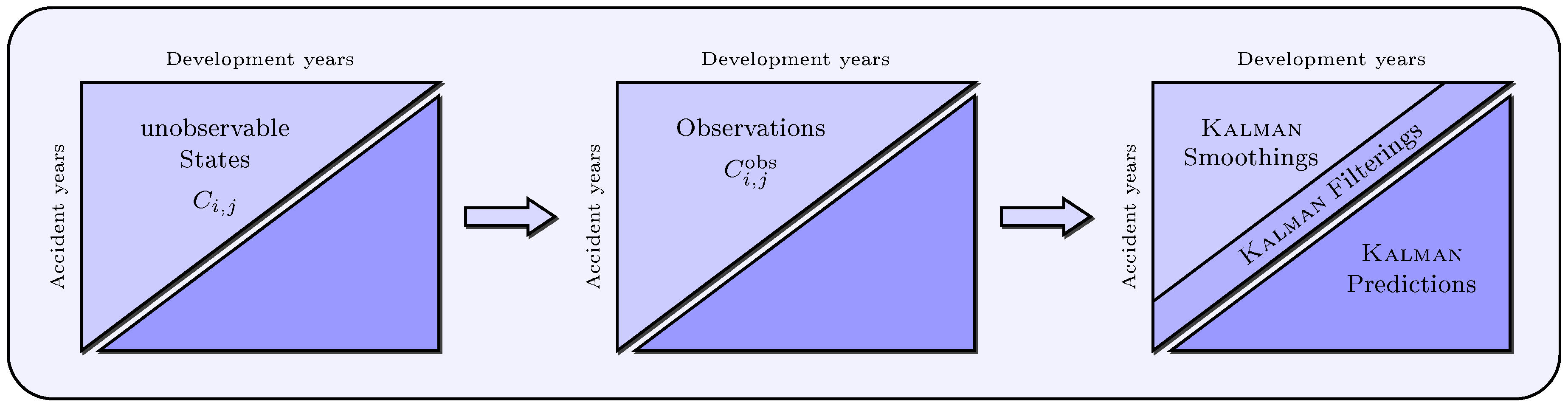
It is assumed that a run-off triangle of observed cumulative payments $C_{i,j}^{\mathrm{obs}}$ is based on a run-off triangle of unobservable states $C_{i,j}$ with $i+j\le I$ for all $i=0,\dots ,I$ and $j=0,\dots ,J$ with $I=J$. Therefore, there is a probable observation error in the claims data, and we can not definitely observe “real cumulative payments”, i.e., the payments made do not necessarily correspond with the payments actually incurred. One possible reason for this difference is that a claim is not reported correctly, for example if the claim is not reported, only partially reported or reported too late. Therefore, we model these unobservable “real cumulative payments” as latent variables. The scalar state space model for cumulative payments presented below provides a basis for determining the entire unobservable upper and lower run-off triangles using Kalman-filter, that is prediction, filtering and smoothing of all states $C_{i,j}$ with $i=0,\dots ,I$ and $j=0,\dots ,J$ (see Figure 3).

Model Assumptions 2

(Scalar state space model for cumulative payments).

⊳

There exist parameters $g_j>0$ and ${\sigma }_w^2>0$, such that:

$$\begin{array}{c}\hfill C_{i,j}^{\mathrm{obs}}=g_j{C}_{i,j}+w_{i,j}(\mathrm{observation}\mathrm{equation})\end{array}$$

(13)

with $w_{i,j}\sim WN\left(0;{\sigma }_w^2\right)$ for $i=0,\dots ,I$ and $j=0,\dots ,J$.

⊳

There exist parameters $f_j>0$ and ${\sigma }_v^2>0$, such that:

$$\begin{array}{c}\hfill C_{i,j+1}=f_j{C}_{i,j}+v_{i,j}(\mathrm{state}\mathrm{equation})\end{array}$$

(14)

with $v_{i,j}\sim WN\left(0;{\sigma }_v^2\right)$ for $i=0,\dots ,I$ and $j=0,\dots ,J-1$.

⊳

The white noise processes ${\left(w_{i,j}\right)}_{j=0,\dots ,J}^{i=0,\dots ,I}$ and ${\left(v_{i,j}\right)}_{j=0,\dots ,J-1}^{i=0,\dots ,I}$ are uncorrelated and therefore satisfy $\mathbb{E}\left[v_{i,j}{w}_{k,l}\right]=0$ for all $i,k=0,\dots ,I$, $j=0,\dots ,J-1$ and $l=0,\dots ,J$.

⊳

Cumulative payments $C_{i,j}$ of different accident years i are stochastically independent.

⊲

The assumption of uncorrelated white noise processes is motivated by the fact that there is no reason to assume a systematic relationship between the measurement noise ${\left(w_{i,j}\right)}_{j=0,\dots ,J}^{i=0,\dots ,I}$ and the process noise ${\left(v_{i,j}\right)}_{j=0,\dots ,J-1}^{i=0,\dots ,I}$. Nevertheless, this assumption is not necessary, but simplifies the Kalman recursions. The further assumption of stochastically independent accident years is frequently applied to claims reserving and especially used in the CL method (see Model Assumptions 1).

The state equation and the observation equation can also be stated as follows:

$$\begin{array}{cc}\hfill C_{i,j}& =f_{j-1}{C}_{i,j-1}+v_{i,j-1}=\dots =a_{i,j}(C_{i,0},v_{i,0},\dots ,v_{i,j-2},v_{i,j-1})\hfill \end{array}$$

(15)

$$\begin{array}{cc}\hfill C_{i,j}^{\mathrm{obs}}& =g_j{C}_{i,j}+w_{i,j}=\dots =b_{i,j}(C_{i,0},v_{i,0},\dots ,v_{i,j-2},v_{i,j-1},w_{i,j})\hfill \end{array}$$

(16)

Here, $a_{i,j}$ and $b_{i,j}$ for $i=0,\dots ,I$ and $j=0,\dots ,J$ are appropriate linear functions. Considering (15), (16) and the assumptions regarding the measurement and process noise, it is clear that:

$$\begin{array}{c}\hfill \mathbb{E}\left[C_{i,j}{v}_{i,l}\right]=0\mathrm{and}\mathbb{E}\left[C_{i,j}{w}_{i,k}\right]=0\end{array}$$

for all $j,k=0,\dots ,J$, $l=0,\dots ,J-1$ with $j\le k$, $j\le l$. Consequently, the initial state $C_{i,0}$ of an accident year $i=0,\dots ,I$ is uncorrelated with $v_{i,j}$ and $w_{i,j}$ for all j.

Remark 1.

• To forecast future cumulative payments $C_{i,j}$ with $i+j>I$ for $i=1,\dots ,I$, $j=1,\dots ,J$ (lower triangle) the corresponding Kalman predictions are required. The one-step predictor provides forecasts for the next calendar year $t=I+1$, while the h-step predictor shall be used for forecasting cumulative payments in calendar years $t=I+h$ with $h>1$.
• As for the underlying states $C_{i,j}$ of the observations $C_{i,j}^{\mathrm{obs}}$ in the upper triangle, the Kalman filterings (for $i+j=I$) and smoothings (for $i+j<I$) are useful to identify outliers in the observations and to replace them with smoothed or filtered observations, as well as to obtain an adjusted presentation of the observed quantities and to determine outlier effects. Another key application of smoothing and filtering is the determination of missing values in the upper run-off triangle (for example, resulting from a merger) to interpolate gaps in the data.

Remark 2.

• We denote the one-step predictor by ${\widehat{C}}_{i,j+1}^{\left(\mathrm{P}\right)}$ and its error variance by ${({\widehat{\sigma }}_{i,j+1}^{\left(\mathrm{P}\right)})}^2=\mathbb{E}[{(C_{i,j+1}-{\widehat{C}}_{i,j+1}^{\left(\mathrm{P}\right)})}^2]$ for $j=0,\dots ,I-i$, as well as the h-step predictor by ${\widehat{C}}_{i,j+h}^{\left(\mathrm{P}\right)}$ and its error variance by ${({\widehat{\sigma }}_{i,j+h}^{\left(\mathrm{P}\right)})}^2=\mathbb{E}[{(C_{i,j+h}-{\widehat{C}}_{i,j+h}^{\left(\mathrm{P}\right)})}^2]$ for $j=0,\dots ,J-h$. The superscript (P) stands for “prediction” and the subscript indicates the cell ($i,j+1$) or ($i,j+h$) in the lower triangle, for which we predict cumulative payments.
• We denote the filtering by ${\widehat{C}}_{i,j}^{\left(\mathrm{F}\right)}$ and its error variance by ${({\widehat{\sigma }}_{i,j}^{\left(\mathrm{F}\right)})}^2=\mathbb{E}[{(C_{i,j}-{\widehat{C}}_{i,j}^{\left(\mathrm{F}\right)})}^2]$ for $j=0,\dots ,I-i$, as well as the smoothings by ${\widehat{C}}_{i,j}^{\left(\mathrm{S}\right)}$ and their error variances by ${({\widehat{\sigma }}_{i,j}^{\left(\mathrm{S}\right)})}^2=\mathbb{E}[{(C_{i,j}-{\widehat{C}}_{i,j}^{\left(\mathrm{S}\right)})}^2]$ for $j=I-i,\dots ,0$. The superscript (F) or (S) stands for “filtering” or “smoothing”, and the subscript indicates the ($i,j$)-cell in the upper triangle, for which we filter or smooth cumulative payments.

The Kalman recursions for prediction, filtering and smoothing are given below. There are two different smoothing approaches: fixed-point and fixed-interval smoothing. While the fixed-point approach calculates smoothed values for a few fixed, predetermined points of time, the fixed-interval approach provides an ex post reconstruction of the behavior of a system in order to understand the phenomenon underlying observations. Since we are going to smooth all observations in the upper run-off triangle for identifying outliers in the data, the fixed-interval algorithm is presented (the fixed-point algorithm can be found for example in Brockwell and Davis (2006)).

Theorem 1 (Kalman-filter algorithms for the scalar state space model).

Given the Model Assumptions 2, the one-step, h-step, filtering and fixed-interval smoothing predictors, as well as their error variances are uniquely determined by the initial conditions ${\widehat{C}}_{i,0}^{\left(P\right)}$ and ${\left({\widehat{\sigma }}_{i,0}^{\left(P\right)}\right)}^2$ and the recursions ($i=0,\dots ,I$, $h\ge 2$):

$$\begin{array}{cccc}\hfill {\widehat{C}}_{i,j+1}^{\left(P\right)}& =f_j{\widehat{C}}_{i,j}^{\left(P\right)}+\frac{f_j{\gamma }_{i,j}}{{\mathrm{\Delta }}_{i,j}}\left(C_{i,j}^{\mathrm{obs}}-g_j{\widehat{C}}_{i,j}^{\left(P\right)}\right)\hfill & \hfill & (j=0,\dots ,I-i)\hfill \end{array}$$

(17)

$$\begin{array}{ccc}\hfill {\widehat{C}}_{i,j+h}^{\left(P\right)}& =(f_{j+h-1}\cdots f_{j+1}){\widehat{C}}_{i,j+1}^{\left(P\right)}\hfill & (j=0,\dots ,J-h)\hfill \end{array}$$

(18)

$$\begin{array}{ccc}\hfill {\widehat{C}}_{i,j}^{\left(F\right)}& ={\widehat{C}}_{i,j}^{\left(P\right)}+\frac{{\gamma }_{i,j}}{{\mathrm{\Delta }}_{i,j}}\left(C_{i,j}^{\mathrm{obs}}-g_j{\widehat{C}}_{i,j}^{\left(P\right)}\right)\hfill & (j=0,\dots ,I-i)\hfill \end{array}$$

(19)

$$\begin{array}{ccc}\hfill {\widehat{C}}_{i,j}^{\left(S\right)}& ={\widehat{C}}_{i,j}^{\left(F\right)}+{\psi }_{i,j}\left({\widehat{C}}_{i,j+1}^{\left(S\right)}-{\widehat{C}}_{i,j+1}^{\left(P\right)}\right)\hfill & (j=I-i,\dots ,0)\hfill \end{array}$$

(20)

and:

$$\begin{array}{ccc}\hfill {\left({\widehat{\sigma }}_{i,j+1}^{\left(P\right)}\right)}^2& =f_j^2{\left({\widehat{\sigma }}_{i,j}^{\left(P\right)}\right)}^2+{\sigma }_v^2-\frac{{\left(f_j{\gamma }_{i,j}\right)}^2}{{\mathrm{\Delta }}_{i,j}}\hfill & (j=0,\dots ,I-i)\hfill \end{array}$$

(21)

$$\begin{array}{ccc}\hfill {\left({\widehat{\sigma }}_{i,j+h}^{\left(P\right)}\right)}^2& =f_{j+h-1}^2{\left({\widehat{\sigma }}_{i,j+h-1}^{\left(P\right)}\right)}^2+{\sigma }_v^2\hfill & (j=0,\dots ,J-h)\hfill \end{array}$$

(22)

$$\begin{array}{ccc}\hfill {\left({\widehat{\sigma }}_{i,j}^{\left(F\right)}\right)}^2& ={\left({\widehat{\sigma }}_{i,j}^{\left(P\right)}\right)}^2-\frac{{\gamma }_{i,j}^2}{{\mathrm{\Delta }}_{i,j}}\hfill & (j=0,\dots ,I-i)\hfill \end{array}$$

(23)

$$\begin{array}{ccc}\hfill {\left({\widehat{\sigma }}_{i,j}^{\left(S\right)}\right)}^2& ={\left({\widehat{\sigma }}_{i,j}^{\left(F\right)}\right)}^2+{\psi }_{i,j}^2\left({\left({\widehat{\sigma }}_{i,j+1}^{\left(S\right)}\right)}^2-{\left({\widehat{\sigma }}_{i,j+1}^{\left(P\right)}\right)}^2\right)\hfill & (j=I-i,\dots ,0)\hfill \end{array}$$

(24)

where ${\gamma }_{i,j}={\left({\widehat{\sigma }}_{i,j}^{\left(P\right)}\right)}^2{g}_j$, ${\mathrm{\Delta }}_{i,j}=g_j^2{\left({\widehat{\sigma }}_{i,j}^{\left(P\right)}\right)}^2+{\sigma }_w^2$ and ${\psi }_{i,j}=f_{j+1}\frac{{\left({\widehat{\sigma }}_{i,j}^{\left(F\right)}\right)}^2}{{\left({\widehat{\sigma }}_{i,j+1}^{\left(P\right)}\right)}^2}$.

⊲

Proof: 

See Appendix A. □

Remark 3.

• The Kalman gain $0\le \frac{{\gamma }_{i,j}}{{\mathrm{\Delta }}_{i,j}}\le 1$ represents the relative importance of the innovation ${\epsilon }_{i,j}=C_{i,j}^{\mathrm{obs}}-g_j{\widehat{C}}_{i,j}^{\left(\mathrm{P}\right)}$ with respect to the prior predictor ${\widehat{C}}_{i,j}^{\left(\mathrm{P}\right)}$. The higher the covariance ${\gamma }_{i,j}$ between the innovation and the state to be predicted and/or the lower the variance ${\mathrm{\Delta }}_{i,j}$ of the innovation, the higher the trust in the new observation $C_{i,j}^{\mathrm{obs}}$ and therefore the higher the Kalman gain.
• Due to the fact that there is no observation after the recent calendar year, and therefore no innovation ${\epsilon }_{i,j}$, the covariance ${\gamma }_{i,j}$ is equal to zero for $i+j>I$. This implies that the Kalman gain is equal to zero in the h-step recursions.
• Since the Kalman smoother is a backwards recursive algorithm and its initializations ${\widehat{C}}_{i,I-i}^{\left(\mathrm{F}\right)}$ and ${\left({\widehat{\sigma }}_{i,I-i}^{\left(\mathrm{F}\right)}\right)}^2$ are values of the last filtering recursion, the smoothings and filterings are identical for the current calendar year $t=I$.

4.2. Determination of Kalman Reserves and MSEP

Using Theorem 1, the ultimate claims $C_{i,J}$ of accident years $i=1,\dots ,I$ can be forecasted. The ultimate claim of the first accident year is predicted by the one-step predictor:

$$\begin{array}{c}\hfill {\widehat{C}}_{1,J}^{\left(\mathrm{P}\right)}=f_{J-1}{\widehat{C}}_{1,J-1}^{\left(\mathrm{P}\right)}+\frac{f_{J-1}{\gamma }_{1,J-1}}{{\mathrm{\Delta }}_{1,J-1}}\left(C_{1,J-1}^{\mathrm{obs}}-g_{J-1}{\widehat{C}}_{1,J-1}^{\left(\mathrm{P}\right)}\right),\end{array}$$

(25)

and the ultimate claims of the accident years $i=2,\dots ,I$ are predicted by the h-step predictors:

$$\begin{array}{c}\hfill {\widehat{C}}_{i,J}^{\left(\mathrm{P}\right)}=(f_{J-1}\cdots f_{J-i+1}){\widehat{C}}_{i,J-i+1}^{\left(\mathrm{P}\right)}.\end{array}$$

(26)

Since we predict the ultimate claims in (26), we have $h=i$. The Kalman reserve ${\widehat{R}}_i$ for a single accident year $i=1,\dots ,I$, as well as the total Kalman reserve $\widehat{R}$ across all accident years can therefore be determined by:

$$\begin{array}{c}\hfill {\widehat{R}}_i={\widehat{C}}_{i,J}^{\left(\mathrm{P}\right)}-C_{i,I-i}^{\mathrm{obs}}\mathrm{and}\widehat{R}=\sum _{i=1}^I{\widehat{R}}_i,\end{array}$$

respectively. The error variance of the predictor ${\widehat{C}}_{1,J}^{\left(\mathrm{P}\right)}$ according to (25) results in:

$$\begin{array}{c}\hfill {\left({\widehat{\sigma }}_{1,J}^{\left(\mathrm{P}\right)}\right)}^2=f_{J-1}^2{\left({\widehat{\sigma }}_{1,J-1}^{\left(\mathrm{P}\right)}\right)}^2+{\sigma }_v^2-\frac{{\left(f_{J-1}{\gamma }_{1,J-1}\right)}^2}{{\mathrm{\Delta }}_{1,J-1}},\end{array}$$

(27)

while the error variances of ${\widehat{C}}_{i,J}^{\left(\mathrm{P}\right)}$ for $i=2,\dots ,I$ according to (26) are given by:

$$\begin{array}{c}\hfill {\left({\widehat{\sigma }}_{i,J}^{\left(\mathrm{P}\right)}\right)}^2=f_{J-1}^2{\left({\widehat{\sigma }}_{i,J-1}^{\left(\mathrm{P}\right)}\right)}^2+{\sigma }_v^2.\end{array}$$

(28)

The error variances (27) and (28) provide a basis for estimating the (unconditional) MSEP. The MSEP for a single accident year $i=1,\dots ,I$ using the Kalman predictor ${\widehat{C}}_{i,J}^{\left(\mathrm{P}\right)}$ is defined as follows:

$$\begin{array}{c}\hfill \mathrm{MSEP}\left({\widehat{C}}_{i,J}^{\left(\mathrm{P}\right)}\right)=\mathbb{E}\left[{\left(C_{i,J}-{\widehat{C}}_{i,J}^{\left(\mathrm{P}\right)}\right)}^2\right]\end{array}$$

Therefore, an appropriate estimator of the MSEP for a single accident year results in:

Definition 1 (Kalman estimator of MSEP for single accident years).

Using Model Assumptions 2 and the Kalman predictor (25) for $i=1$ or (26) for $i=2,\dots ,I$ at time $t=I$, an estimator of the MSEP for a single accident year $i=1,\dots ,I$ is given by:

$$\begin{array}{c}\hfill \widehat{\mathrm{MSEP}}\left({\widehat{C}}_{i,J}^{\left(P\right)}\right)={\left({\widehat{\sigma }}_{i,J}^{\left(P\right)}\right)}^2\end{array}$$

⊲

To determine an estimator of the MSEP for aggregated accident years, we consider two different accident years $i,k=1,\dots ,I$ with $i<k$ in the first step.

$$\begin{array}{cc}\hfill \mathrm{MSEP}\left({\widehat{C}}_{i,J}^{\left(\mathrm{P}\right)}+{\widehat{C}}_{k,J}^{\left(\mathrm{P}\right)}\right)& =\mathbb{E}\left[{\left(C_{i,J}-{\widehat{C}}_{i,J}^{\left(\mathrm{P}\right)}+C_{k,J}-{\widehat{C}}_{k,J}^{\left(\mathrm{P}\right)}\right)}^2\right]\hfill \\ & =\mathbb{E}\left[{\left(C_{i,J}-{\widehat{C}}_{i,J}^{\left(\mathrm{P}\right)}\right)}^2\right]+\mathbb{E}\left[{\left(C_{k,J}-{\widehat{C}}_{k,J}^{\left(\mathrm{P}\right)}\right)}^2\right]\hfill \\ & +2\mathbb{E}\left[\left(C_{i,J}-{\widehat{C}}_{i,J}^{\left(\mathrm{P}\right)}\right)\left(C_{k,J}-{\widehat{C}}_{k,J}^{\left(\mathrm{P}\right)}\right)\right]\hfill \\ & =\mathrm{MSEP}\left({\widehat{C}}_{i,J}^{\left(\mathrm{P}\right)}\right)+\mathrm{MSEP}\left({\widehat{C}}_{k,J}^{\left(\mathrm{P}\right)}\right)\hfill \\ & +2\mathbb{E}\left[\left(C_{i,J}-{\widehat{C}}_{i,J}^{\left(\mathrm{P}\right)}\right)\left(C_{k,J}-{\widehat{C}}_{k,J}^{\left(\mathrm{P}\right)}\right)\right]\hfill \end{array}$$

(29)

Therefore, the MSEP for two accident years is the sum of two single accident year MSEPs and a mixed term based on both accident years. Using independence of the different accident years (see Model Assumptions 2), we obtain for the expectation in (29):

$$\begin{array}{cc}\hfill \mathbb{E}\left[\left(C_{i,J}-{\widehat{C}}_{i,J}^{\left(\mathrm{P}\right)}\right)\left(C_{k,J}-{\widehat{C}}_{k,J}^{\left(\mathrm{P}\right)}\right)\right]& =\mathbb{E}\left[C_{i,J}-{\widehat{C}}_{i,J}^{\left(\mathrm{P}\right)}\right]\mathbb{E}\left[C_{k,J}-{\widehat{C}}_{k,J}^{\left(\mathrm{P}\right)}\right]\hfill \\ & =\left(\mathbb{E}\left[C_{i,J}\right]-\mathbb{E}\left[{\widehat{C}}_{i,J}^{\left(\mathrm{P}\right)}\right]\right)\left(\mathbb{E}\left[C_{k,J}\right]-\mathbb{E}\left[{\widehat{C}}_{k,J}^{\left(\mathrm{P}\right)}\right]\right)\hfill \end{array}$$

(30)

Since ${\widehat{C}}_{i,J}^{\left(\mathrm{P}\right)}$ is an unbiased predictor for the ultimate claim $C_{i,J}$, the term (30) is equal to zero. Consequently, the MSEP for two accident years results from the sum of two single accident year MSEPs:

$$\begin{array}{c}\hfill \mathrm{MSEP}\left({\widehat{C}}_{i,J}^{\left(\mathrm{P}\right)}+{\widehat{C}}_{k,J}^{\left(\mathrm{P}\right)}\right)=\mathrm{MSEP}\left({\widehat{C}}_{i,J}^{\left(\mathrm{P}\right)}\right)+\mathrm{MSEP}\left({\widehat{C}}_{k,J}^{\left(\mathrm{P}\right)}\right)\end{array}$$

The MSEP of all considered accident years is therefore, by independence, determined as:

$$\begin{array}{c}\hfill \mathrm{MSEP}\left(\sum _{i=1}^I{\widehat{C}}_{i,J}^{\left(\mathrm{P}\right)}\right)=\sum _{i=1}^I\mathrm{MSEP}\left({\widehat{C}}_{i,J}^{\left(\mathrm{P}\right)}\right)\end{array}$$

Thus, an estimator of the MSEP for aggregated accident years is given by:

Definition 2 (Kalman estimator of MSEP for aggregated accident years).

Using Model Assumptions 2, we have the following estimator for the MSEP of the ultimate claim for aggregated accident years:

$$\begin{array}{c}\hfill \widehat{\mathrm{MSEP}}\left(\sum _{i=1}^I{\widehat{C}}_{i,J}^{\left(P\right)}\right)=\sum _{i=1}^I\widehat{\mathrm{MSEP}}\left({\widehat{C}}_{i,J}^{\left(P\right)}\right)\end{array}$$

⊲

5. Empirical Applications

In this section, various empirical applications are considered. The applications are based on the claims development triangle of Taylor and Ashe (1983) (see Table 1). Firstly, the scalar state space model is used to calculate predicted, filtered and smoothed values for cumulative payments, as well as outlier effects in the data. Secondly, an empirical comparison of representative state space models and other popular methods in claims reserving is made.

5.1. Applications of Scalar State Space Model

Using Theorem 1, we can calculate forecasts, as well as filtered and smoothed cumulative payments, but in a prior step, we need to estimate the model parameters $g_j$, $f_j$, ${\sigma }_w^2$, ${\sigma }_v^2$ and the initializations ${\widehat{C}}_{i,0}^{\left(\mathrm{P}\right)}$ and ${\left({\widehat{\sigma }}_{i,0}^{\left(\mathrm{P}\right)}\right)}^2$ for all $i,j$. Alternatively, they can also be determined by consulting expert opinion, market statistics or similar portfolios. In this section, we estimate the parameters as follows. Taking conditional expectations of both sides of (14) with respect to $C_{i,j}$ leads directly to $\mathbb{E}\left[C_{i,j+1}\right|C_{i,j}]=f_j{C}_{i,j}$. If we compare this result to (1), we find that $f_j$ plays the role of the usual CL factor. This fact motivates the estimation of the factors $f_0,\dots ,f_{J-1}$ using the CL estimator (2). To avoid over-parametrization of the model, the parameter $g_j=g$ is assumed to be time-invariant. The parameters g, ${\sigma }_w^2$, ${\sigma }_v^2$ are estimated using maximum likelihood (ML) method in conjunction with the expectation-maximization (EM) algorithm. Since a direct maximization of the Gaussian log likelihood can cause local maxima or convergence problems, we use the EM algorithm, which is an iterative method to find ML estimates based on the expected conditional Gaussian log likelihood (for more details on the EM algorithm, see Shumway and Stoffer (1982), Shumway and Stoffer (2010) or Johannssen (2016)).

Taking the observations $C_{i,0}^{\mathrm{obs}}$ in the respective accident years $i=0,\dots ,I$ and the CL variance parameter ${\widehat{\sigma }}_0^2$ (see (3)) as initializations, we get the following parameter estimates for the run-off triangle of Taylor and Ashe (1983) in

Table 2. Estimated parameter values for the dataset of Taylor and Ashe (1983).

${\widehat{\mathit{f}}}_0$	${\widehat{\mathit{f}}}_1$	${\widehat{\mathit{f}}}_2$	${\widehat{\mathit{f}}}_3$	${\widehat{\mathit{f}}}_4$	${\widehat{\mathit{f}}}_5$	${\widehat{\mathit{f}}}_6$	${\widehat{\mathit{f}}}_7$	${\widehat{\mathit{f}}}_8$	$\widehat{\mathit{g}}$
3.4906	1.7473	1.4574	1.1739	1.1038	1.0863	1.0539	1.0766	1.0177	1.0014

:

Since individual estimates of g for different years slightly deviate between $0.98$ and $1.02$, the assumption of time invariance has no significant impact on the calculated results. On the contrary: Due to the small number of observations in more recent years, the quality of the respective estimates would be questionable. Moreover, the estimated value $\widehat{g}\approx 1$ suggests the presumption for the dataset of Taylor and Ashe (1983) that the observations do not differ systematically upwards or downwards from the underlying states.

The predicted, filtered and smoothed cumulative payments are given in

Table 3. Predictions (lower triangle), Filterings (last diagonal of upper triangle), Smoothings (upper triangle) for the data set of Taylor and Ashe (1983).

Accident	Development Year j
Year i	0	1	2	3	4	5	6	7	8	9
0	357846	1088646	1724703	2344677	2801926	3216482	3460558	3608732	3849709	3907933
1	352118	1245805	2202664	3283457	3811445	4186179	4624394	4910422	5318601	5412740
2	290510	1218431	2204841	3256998	3888722	4213313	4619217	4892887	5267683	5360921
3	310611	1301186	2304955	3558299	4046805	4374444	4652591	4903365	5278963	5372401
4	443156	1255658	2103481	2949026	3444357	3845121	4176955	4402093	4739293	4823179
5	396131	1303545	2175261	3073819	3659435	4039284	4387874	4624381	4978608	5066730
6	440830	1384198	2411162	3494015	4101625	4527373	4918086	5183170	5580201	5678971
7	359483	1455238	2750622	4008757	4705880	5194350	5642622	5946760	6402282	6515602
8	376686	1344075	2348503	3422708	4017917	4434977	4817715	5077390	5466318	5563072
9	344014	1200815	2098185	3057894	3589662	3962269	4304213	4536210	4883683	4970125

.

Using the smoothed values ${\widehat{C}}_{i,j}^{\left(\mathrm{S}\right)}$ for $i+j\le 9$ (upper triangle in Table 3), outliers in the data can be identified in the first place. Subsequently, outlier effects can be isolated, and observations can be robustified.

Table 4. Kalman outlier effects.

Accident	Development Year j
Year i	0	1	2	3	4	5	6	7	8	9
0	2	36142	10627	$-126407$	$-56330$	103512	5778	$-2446$	$-16194$	$-6470$
1	0	$-9666$	$-32631$	69865	$-12378$	$-66116$	23473	3617	20484
2	$-3$	73875	13684	$-21819$	97273	$-80395$	9693	16428
3	$-3$	117672	$-109908$	199148	$-16876$	7538	$-64323$
4	4	$-119308$	24852	$-51205$	$-41685$	28190
5	1	29672	5454	$-88067$	32277
6	2	$-95735$	8699	$-10885$
7	$-3$	$-34110$	113876
8	0	19219
9	0

shows the outlier effects ${\widehat{Z}}_{i,j}=C_{i,j}^{\mathrm{obs}}-{\widehat{C}}_{i,j}^{\left(\mathrm{S}\right)}$ for all $i=0,\dots ,9$ and $j=0,\dots ,9-i$.

The outlier effects at $j=0$ are negligible or equal to zero for all $i=0,\dots ,9$ due to the chosen initializations. As for the magnitude of the observed cumulative payments, the outlier effects are relatively minor with a few exceptions. The largest outlier effect ${\widehat{Z}}_{3,3}$ has an (absolute) deviation of 199148. For example, the outlier effect ${\widehat{Z}}_{0,9}=-6470$ indicates that we have an observation error in the data, which implies that the cumulative payments made are way too low compared to the unobservable “real cumulative payments”, i.e., there are still outstanding payments. It is for some claims reserving methods (such as the CL method), which are not robust against outliers, of high relevance, if the observations $C_{i,I-i}^{\mathrm{obs}}$ for $i=1,\dots ,I$ of the current calendar year represent outliers. Therefore, two cumulative payments $C_{3,6}^{\mathrm{obs}}$ and $C_{7,2}^{\mathrm{obs}}$ in the run-off triangle of Taylor and Ashe (1983) should be treated with caution. In particular, such observations should be robustified, for example, they could be replaced by the Kalman smoothed values. As for the Kalman recursion algorithms, outliers entail less problems because of the lack of credibility of these observations and, consequently, the minor Kalman gain, i.e., outliers do not change the forecast decisively.

The robustness of the CL method and the impact of outliers were also considered by Verdonck et al. (2009), who primarily surveyed how (simulated) outliers affect the CL total reserve. The results of their study show that the most problematic areas in a run-off triangle are the lower left corner and the upper right corner, since there are too few observations. In these areas, the CL method is particularly sensitive to outliers, because the CL reserves directly and indirectly (via the CL estimators (2)) depend on the observations of the recent calendar year. Further papers on the subject of robustness of the CL method are, for example, Van Wouwe et al. (2009), Verdonck and Debruyne (2011) and Verdonck and Van Wouwe (2011).

5.2. Empirical Comparison of Selected Models

The models considered in the empirical comparison are the scalar state space model, but the models in Verrall (1989), Alpuim and Ribeiro (2003), Li (2006), Atherino et al. (2010) and the well-known methods CL and Bornhuetter–Ferguson (BF), as well as the (overdispersed) Poisson (ODP) model. The chosen BF method is rather conservative, i.e., we use a priori estimates for the expected ultimate claims, which generally exceed estimates based on development triangle data. It should be pointed out that the BF results depend largely on the quality of the a priori estimates.

The most results in

Table 5. Reserves, standard errors and VCOs for selected models.

i	Scalar State Space Model			Verrall (1989)
	Reserve	$\sqrt{\mathbf{MSEP}}$	$\mathbf{VCO}$	Reserve	$\sqrt{\mathbf{MSEP}}$	$\mathbf{VCO}$
1	73655	167499	227.4%	143834	72675	50.5%
2	451606	221667	49.1%	465847	166438	35.7%
3	784133	270524	34.5%	673175	194229	28.9%
4	949868	317331	33.4%	1060794	266228	25.1%
5	1375018	366006	26.6%	1479407	339755	23.0%
6	2195841	422159	19.2%	2218738	487975	22.0%
7	3651104	507337	13.9%	3287633	735669	22.4%
8	4199778	662654	15.8%	4517179	1040596	23.0%
9	4626111	797161	17.2%	4570683	1167068	25.5%
aggr.	18307113	1376670	7.5%	18417290	2627190	14.3%
$\mathit{i}$	Alpuim and Ribeiro (2003)			Atherino et al. (2010)
	Reserve	$\sqrt{\mathbf{MSEP}}$	$\mathbf{VCO}$	Reserve	$\sqrt{\mathbf{MSEP}}$	$\mathbf{VCO}$
1	66860	161177	241.1%	78904	18385	23.3%
2	321421	227246	70.7%	433790	75046	17.3%
3	551625	278017	51.0%	663312	90874	13.7%
4	1243900	322745	25.9%	891774	107013	12.0%
5	1535502	422709	27.5%	1336361	144327	10.8%
6	2356440	625125	26.5%	2009913	207021	10.3%
7	2817779	1667381	59.2%	2919587	303637	10.4%
8	4472888	1448251	32.4%	3810769	411563	10.8%
9	4942889	763241	15.4%	4726935	571959	12.1%
aggr.	18309304	1637284	8.9%	16871345	1197865	7.1%
$\mathit{i}$	Li (2006)			BF Method
	Reserve	$\sqrt{\mathbf{MSEP}}$	$\mathbf{VCO}$	Reserve	$\sqrt{\mathbf{MSEP}}$	$\mathbf{VCO}$
1	101374	54755	54.0%	104097	117241	112.6%
2	457788	178242	38.9%	516462	218187	42.2%
3	651123	198744	30.5%	780602	255401	32.7%
4	1035739	271135	26.2%	1083378	284276	26.2%
5	1473338	360715	24.5%	1561405	334286	21.4%
6	2190410	522967	23.9%	2395405	409247	17.1%
7	3442432	808061	23.5%	4312331	550065	12.8%
8	4269816	1054731	24.7%	4706870	560833	11.9%
9	5027791	1425522	28.4%	5088393	578565	11.4%
aggr.	18649811	2809220	15.1%	20548942	1220525	5.9%
$\mathit{i}$	CL Method			ODP Model
	Reserve	$\sqrt{\mathbf{MSEP}}$	$\mathbf{VCO}$	Reserve	$\sqrt{\mathbf{MSEP}}$	$\mathbf{VCO}$
1	94634	75535	79.8%	94634	110100	116.3%
2	469511	121700	25.9%	469511	216043	46.0%
3	709638	133551	18.8%	709638	260872	36.8%
4	984889	261412	26.5%	984889	303550	30.8%
5	1419459	411028	29.0%	1419459	375014	26.4%
6	2177641	558356	25.6%	2177641	495378	22.7%
7	3920301	875430	22.3%	3920301	789961	20.2%
8	4278972	971385	22.7%	4278972	1046514	24.5%
9	4625811	1363385	29.5%	4625811	1980101	42.8%
aggr.	18680856	2447618	13.1%	18680856	2945661	15.8%

suggest total claims reserves of approximately $18500000\pm 200000$. The model in Atherino et al. (2010) and the conservative BF method present differing results with more optimistic and more conservative total reserves, respectively. Higher reserves tend to lead to higher MSEP, just like in the ODP model, Li (2006), Verrall (1989) and the CL method, with the exception of the BF method and the scalar state space model. The model of Atherino et al. (2010), which provides by far the lowest total claims reserves, also leads to the smallest MSEP for aggregated accident years, but not to the smallest variational coefficient ($\mathrm{VCO}=\sqrt{\mathrm{MSEP}}/\mathrm{reserve}$) for aggregated accident years.

The conservative BF method produces the smallest VCO for aggregated accident years, closely followed by Atherino et al. (2010), the scalar state space model and Alpuim and Ribeiro (2003). The model of Alpuim and Ribeiro (2003) and the scalar state space model provide a large VCO in the first accident year, resulting from the interaction of relatively low reserves and a larger MSEP for this year. In particular, for the scalar state space model the VCO decreases noticeably in subsequent accident years. Other models, like the log-normal models in Verrall (1989) and Li (2006), lead to relatively low VCO in the first accident years, but without a remarkable reduction in later accident years, so they remain mostly at the level of $25\%\pm 3\%$.

Compared with the results of the other seven models, the scalar state space model produces quite precise results with relatively low MSEPs and VCOs. Thus, the scalar structure of this model leads not only to facilitated practical application, but it is also in no way inferior to more complex models for the considered dataset.

6. Conclusions

The previously written papers in the stochastic claims reserving literature based on state space models and the Kalman-filter have numerous contentual similarities, and we can classify them into four categories related to the methodology or modeling used in the respective papers. Models for incremental payments dominate in this field of research, in particular variations on the Hoerl curve, the log-normal model, as well as calendar year-based state space representations. However, most state space representations in these papers entail a matrix-based approach, which complicates their direct application in practice.

In contrast, the newly-developed scalar state space model for cumulative payments is quite elegant due to its simple, yet powerful structure. Since the CL method is the most commonly-used reserving method in practice and the scalar state space model is an extension of the CL method, the scalar state space model can readily be applied to claims reserving practice. In particular, this model provides facilitated calculation of forecasts for the cumulative payments in the lower run-off triangle and of smoothed values for the cumulative payments in the upper triangle. Moreover, the determination of claims reserves and the estimation of their MSEP for single and aggregated accident years are straightforward calculations using Kalman-filter. The scalar state space model can also be used to identify and smooth outliers. This subject is of particular importance for less robust claims reserving methods such as the CL method. Summarizing, the scalar state space model is a very promising, robustified extension of the CL method, which renounces a complex matrix structure compared to most state space models in claims reserving and therefore simplifies its practical applications.

Because of its recursive and dynamic nature, the Kalman-filter is predestined for use in stochastic claims reserving. The authors McGuire (2007), Taylor and McGuire (2008) and Chima-Okereke (2013) even recommend the use of state space models as a part of a nearly completely automated script, a so-called reserving robot in stochastic claims reserving. Due to the high flexibility of state space models and the Kalman-filter, it is also possible to perform multivariate analyses in a simple manner and to take several run-off triangles simultaneously into account. In this way, dependencies, in particular correlations, between run-off triangles can be surveyed and included into the modeling.

References

- Alpuim, Teresa, and Isabel Ribeiro. 2003. A State Space Model for Run-Off Triangles. Applied Stochastic Models in Business and Industry 19: 105–20. [Google Scholar] [CrossRef]
- Atherino, Rodrigo, Adrian Pizzinga, and Cristiano Fernandes. 2010. A row-wise Stacking of the Runoff Triangle: State Space Alternatives for IBNR Reserve Prediction. ASTIN Bulletin 40: 917–46. [Google Scholar]
- Brockwell, Peter J., and Richard A. Davis. 2006. Time Series: Theory and Methods, 2nd ed. New York: Springer. [Google Scholar]
- Chima-Okereke, Chibisi. 2013. A practical Approach to Claims Reserving using State Space Models with Growth Curves. Paper presented at the R in Insurance Conference 2013, London, UK, July 15. [Google Scholar]
- De Jong, Piet. 2005. State Space Models in Actuarial Science. Paper presented at the Second Brazilian Conference on Statistical Modelling in Insurance, Institute of Mathematics and Statistics, University of São Paulo, Maresias, Brazil, August 28–September 3. [Google Scholar]
- De Jong, Piet. 2006. Forecasting Runoff Triangles. North American Actuarial Journal 10: 28–38. [Google Scholar] [CrossRef]
- De Jong, Piet, and Ben Zehnwirth. 1983. Claims Reserving, State-Space Models and the Kalman Filter. Journal of the Institute of Actuaries 110: 157–81. [Google Scholar] [CrossRef]
- England, Peter D., and Richard J. Verrall. 2002. Stochastic Claims Reserving in General Insurance. British Actuarial Journal 8: 443–518. [Google Scholar] [CrossRef]
- Frees, Edward W. 2010. Regression Modeling with Actuarial and Financial Applications. Cambridge: Cambridge University Press. [Google Scholar]
- Johannssen, Arne. 2016. Stochastische Schadenreservierung unter Verwendung von Zustandsraummodellen und des Kalman-Filters. Hamburg: Dr. Kovac. [Google Scholar]
- Kaas, Rob, Marc Goovaerts, Jan Dhaene, and Michel Denuit. 2009. Modern Actuarial Risk Theory—Using R, 2nd ed. Berlin: Springer. [Google Scholar]
- Kalman, Rudolf E. 1960. A New Approach to Linear Filtering and Prediction Problems. Trans. of the ASME—Journal of Basic Engineering (Series D) 82: 35–45. [Google Scholar] [CrossRef]
- Kremer, Erhard. 1982. IBNR-Claims and the Two-Way Model of ANOVA. Scandinavian Actuarial Journal 1982: 47–55. [Google Scholar] [CrossRef]
- Li, Jackie. 2006. Comparison of Stochastic Reserving Methods. Australian Actuarial Journal 12: 489–569. [Google Scholar]
- Mack, Thomas. 1993. Distribution-free Calculation of the Standard Error of Chain Ladder Reserve Estimates. ASTIN Bulletin 23: 213–25. [Google Scholar] [CrossRef]
- McGuire, Gráinne. 2007. Building a Reserving Robot. Paper presented at the Biennial Convention 2007, Institute of Actuaries of Australia, Christchurch, New Zealand, September 23–26. [Google Scholar]
- Ntzoufras, Ioannis, and Petros Dellaportas. 2002. Bayesian Modelling of Outstanding Liabilities incorporating Claim Count Uncertainty. North American Actuarial Journal 6: 113–28. [Google Scholar] [CrossRef]
- Pang, Liyan, and Siqi He. 2012. The Application of State-Space Model in Outstanding Claims Reserve. Paper presented at the 2012 International Conference on Information Management, Innovation Management and Industrial Engineering (ICIII), Sanya, China, October 20–21; pp. 271–74. [Google Scholar]
- Shumway, Robert H., and David S. Stoffer. 1982. An Approach to Time Series Smoothing and Forecasting using the EM Algorithm. Journal of Time Series Analysis 3: 253–64. [Google Scholar] [CrossRef]
- Shumway, Robert H., and David S. Stoffer. 2010. Time Series Analysis and Its Applications (With R Examples), 3rd ed. New York: Springer. [Google Scholar]
- Taylor, Greg C. 2000. Loss Reserving: An Actuarial Perspective. Boston: Kluwer Academic Publishers. [Google Scholar]
- Taylor, Greg C., and Frank R. Ashe. 1983. Second Moments of Estimates of Outstanding Claims. Journal of Econometrics 23: 37–61. [Google Scholar] [CrossRef]
- Taylor, Greg C., and Gráinne McGuire. 2008. Robotic Reserving. GIRO Convention 2013, Italy. [Google Scholar]
- Taylor, Greg C., Gráinne McGuire, and Alan Greenfield. 2003. Loss Reserving: Past, Present and Future. Research Paper No. 109. Melbourne: University of Melbourne. [Google Scholar]
- Van Wouwe, Martine, Tim Verdonck, and Kristel Van Rompay. 2009. Application of Classical and Robust Chain-Ladder Methods: Results for the Belgian Non-Life Business. Global Business and Economics Review 11: 99–115. [Google Scholar] [CrossRef]
- Verdonck, Tim, and Michiel Debruyne. 2011. The Influence of Individual Claims on the Chain-Ladder Estimates: Analysis and Diagnostic Tool. Insurance: Mathematics and Economics 48: 85–98. [Google Scholar] [CrossRef]
- Verdonck, Tim, and Martine Van Wouwe. 2011. Detection and Correction of Outliers in the Bivariate Chain-Ladder Method. Insurance: Mathematics and Economics 49: 188–93. [Google Scholar] [CrossRef]
- Verdonck, Tim, Martine Van Wouwe, and Jan Dhaene. 2009. A Robustification of the Chain-Ladder Method. North American Actuarial Journal 13: 280–98. [Google Scholar] [CrossRef]
- Verrall, Richard J. 1989. A State Space Representation of the Chain Ladder Linear Model. Journal of the Institute of Actuaries 116: 589–610. [Google Scholar] [CrossRef]
- Verrall, Richard J. 1994. A Method for Modelling Varying Run-off Evolutions in Claims Reserving. ASTIN Bulletin 24: 325–32. [Google Scholar] [CrossRef]
- Verrall, Richard J. 2004. Kalman Filter, Reserving Methods. In Encyclopedia of Actuarial Science. Edited by J. L. Teugels and B. Sundt. Chichester: John Wiley & Sons, vol. 1, pp. 952–55. [Google Scholar]
- Wright, Thomas S. 1990. A Stochastic Method for Claims Reserving in General Insurance. Journal of the Institute of Actuaries 117: 677–731. [Google Scholar] [CrossRef]
- Wüthrich, Mario V., and Michael Merz. 2008. Stochastic Claims Reserving Methods in Insurance. Chichester: John Wiley & Sons. [Google Scholar]
- Zehnwirth, Ben. 1997. Kalman Filters with Applications to Loss Reserving. Insurance: Mathematics and Economics 20: 149–218. [Google Scholar]
Figure 1.
Chronology and categorization of the papers based on state space models.
Figure 2.
Modeling approaches of claims development data.
Figure 3.
Unobservable states, observations and Kalman smoothings (), Kalman filterings () and Kalman predictions ().