Abstract
Little in the scholarly economics literature is directed specifically to the performance of stable value funds, although they occupy a leading place among retirement investment vehicles. They are currently offered in more than one-third of all defined contribution plans in the USA, with more than $800 billion of assets under management. This paper rigorously examines their performance throughout the entire period since their inception in 1973. We produce a composite index of stable value returns. We next conduct mean-variance analysis, Sharpe and Sortino ratio analysis, stochastic dominance analysis, and optimal multi-period portfolio composition analysis. Our evidence suggests that stable value funds dominate (on average) two major asset classes based on a historical analysis, and that they often occupy a significant position in optimized portfolios across a broad range of risk aversion levels. We discuss factors that contributed to stable value funds’ past performance and whether they can continue to perform well into the future. We also discuss considerations regarding whether or not to include stable value as an element in target date funds within defined contribution pension plans.
1. Introduction
In this updated study,1 we reexamine the past history of stable value (SV) funds and their performance over the past 43 years, with particular emphasis on the past 27 years. A growing volume of industry and practitioner research has provided a detailed look at how the funds are managed and stable values secured.2 Additionally, academic articles increasingly are including SV funds within the purview of their studies,3 although it is difficult to find in-depth scholarly treatments of SV funds performance outside of our preliminary working papers.4 The lack of rigorous performance studies is rather surprising because SV funds occupy such a prominent place among retirement investment vehicles, with over $800 billion of assets under management.5 That puts them roughly on par with the increasingly popular target-date funds, which reportedly held some $880.4 billion of assets under management as of the end of 2016.6 SV funds are offered as an investment option in over one-third of all defined contribution (DC) plans, including 457, 403(b), 401(k) and some Section 529 Tuition Assistance Plans. By February 2009, they peaked at 36.7% of their assets due primarily to stock market declines, although allocations are more typically within the 10–25% range.7 More ironically, the lack of performance analyses did not forestall an onslaught of articles criticizing stable value and advocating that plan participants downsize their allocations toward the SV options (e.g., (GAO 2011)).
In this updated study, we provide a rigorous analysis of the performance of SV funds, enlisting an extended data set that goes from 1973 through 2015. We also include SV return data through the end of 2016 for informational purposes only.8 We compare their performance to that of basic asset classes such as U.S. large and small stocks, long-term government and corporate bonds, intermediate-term government bonds, and money market funds, using three methods: mean- variance analysis, stochastic dominance analysis, and an enhanced multiperiod utility analysis. Our study shows that since the inception of stable funds in late 1988, and their precursors in 1973, none of these other asset classes has dominated them; on the contrary, SV funds have dominated money market and intermediate-term government bond funds (and nearly dominated long-term corporate bonds as well) over a wide range of risk aversion levels and, when combined with small stocks and long-term government bonds, they occupy a prominent and often dominant part in optimal portfolios.9
Before concluding our study, we explain the value proposition for SV funds—how they have been able to generate notable returns for their investors—and whether the contributors to their past performance can be expected to continue into the future. We consider the recent financial crisis and revisit how the funds have weathered that crisis. We comment briefly on the themes and considerations of plan sponsors and their fiduciaries who choose not to include SV funds in their menus of options for plan participants and consider complications for incorporating SV in the increasingly popular target date funds.
2. Background
Stable value funds are labeled in various ways, including Capital Accumulation, Principal Protection, Guaranteed, Preservation, Income funds, as well as Guaranteed Investment Contracts (GICs) and Group Annuity Contracts, among others. Early forms of SV funds have been around since the 1970s, coinciding with the development of U.S. defined contribution (DC) plans. From their outset, these funds consisted largely of laddered maturity GICs issued by insurance companies. Return of principal and periodically-reset interest rates over a certain period of time were guaranteed regardless of the performance of the underlying assets. Both principal and interest were fully backed by the GIC issuer’s general account. Over time, some plan sponsors sought an alternative structure that would provide them with greater flexibility and control, as the assets backing the GIC contracts were owned and managed by the insurer and the underlying investment strategy was that of the insurer’s general account.
Such concerns were addressed, in part, with the creation in late 1988 of separate account GICs, where the assets underlying the contracts, although still owned by the insurance company, were held in separate accounts for the exclusive benefit of the plan(s) participating in the separate account and could not be used to discharge claims against the general account of the insurer. In this structure, the guarantees against any investment shortfalls stemming from poor performance of the separate account assets were still secured by assets in the general account and surplus. This innovation provided additional flexibility to fund managers, who could pursue a customized investment strategy rather than a general account investment strategy.
Then, in the early 1990s, the SV funds market broadened when synthetic GICs (initially called Trust GICs) were created in an effort to allow plans to retain legal title to plan assets, and to provide additional flexibility in terms of investment strategy and asset selection. This structure enabled non-insurers to manage the plan assets, which are directly owned by the participating plan(s), while the financial protections were secured by banks, insurers, and other financial institutions. Today, synthetic GICs occupy a prominent position in stable value, and coexist with traditional and separate account GICs.10 Each structure of stable value carries features that are preferable to different plan sponsors. Some prefer the yields and generous plan administration fee offsets that may be available through general account GIC-based plans; others prefer the investment flexibility of separate account GICs, while still others seek the underlying asset ownership feature of synthetic GIC-based funds. The driving factor underlying the choice of SV structure would be what is suitable for plan participants.
A stable value fund offers principal protection and liquidity to individual investors, and steady returns that are roughly comparable to intermediate-term bond yields, but do not exhibit the volatility of intermediate-term bond total rates of return. Additionally, over ensuing one-to-six- month intervals (depending on the SV contract), the guaranteed rate of return moves more slowly than intermediate-term bond yields. This is achieved by having a process and investment contract, discussed in the following section, that allow the provider to smooth market volatility through amortizing gains and losses over the duration of the portfolio. This smoothing is effected through crediting rate reset mechanisms and protocols that insulate investors against day-to-day volatility. As a consequence of these features and the underlying short-to-intermediate-term fixed income investments, SV funds provide investors with positive returns of very low volatility. This combination of bond-yield-like returns and low volatility obtains contract or book value accounting of the investment.11
The underlying investment portfolios of all three forms of stable value funds typically comprise high quality, short maturity (usually under seven years) corporate and government bonds, mortgage-backed securities, asset-backed securities, and other structured products. In the case of synthetics, the portfolio is protected against interest rate risk through an investment contract obtained from a high quality bank, insurer or other financial institution. This means that in all but a few prespecified circumstances, investors in an SV fund are able to transact (make deposits, withdrawals, transfers) at book or contract value, which is deposits plus accrued interest, less any past withdrawals. In financial industry jargon, this is known as “benefit responsiveness.”
Stable value funds do not require a set holding period but provide participants full access to their principal and accumulated interest without a penalty. However, they are subject to general restrictions within the overall plan. For example, many plans restrict participants from the direct transfer to a competing short-duration bond or money market fund by requiring that money transferred out of SV first be invested in a non-competing (e.g., stock or long-term bond) fund for a short period such as 30–90 days to eliminate arbitrage trading. This rule, together with the fact that plan participants do not act in concert regarding the allocation of their funds, allow the investment contract protections to be purchased for a fraction of what it would cost if interest arbitrageurs pervaded the pool and were revising their allocations aggressively.
3. Crediting Rate Formula
From an investor’s viewpoint, SV funds operate somewhat like a passbook savings account. They accrue interest at a prespecified crediting rate that is generally updated periodically (every one to six months, in accordance with investment contract specifications) to incorporate changing market conditions. Their principal is secure and grows over time by the amounts of interest credited to their account. Crediting rates on SV funds change more slowly than bond yields and may be guided according to a formula which basically produces an internal rate of return for the investment by requiring that the contract (or book) value of the portfolio converge to its market value by the end of the assumed duration. We define the variables in the formula as follows:
- CR: crediting rate applied to the accounts of investors in the SV funds
- MV: market value of the underlying portfolio
- CV: contract value of the underlying portfolio
- D: duration of the underlying portfolio or duration of a benchmark portfolio
- Y: yield of the underlying portfolio, as described further below.
Given these variables, the future market value (FMV) of the portfolio is given by
The crediting rate that guarantees this value, given the current contract value, is the solution to
Therefore, the crediting rate formula is given by equating the right-hand-side of Expressions (1) and (2), and solving for CR,
Although other variations of the crediting rate formula are also used for guidance, expression (3) is the one most generally used (see SVIA 2005, p. 4). In addition to small differences in the crediting rate formulae, managers do not always calculate the inputs to the formulae in the same way. For example, with respect to the measure of duration D, some fund managers use the duration of a benchmark portfolio, while others use the duration of the underlying securities. The yield measure Y is most often a duration market-weighted bond equivalent yield, although some variations have occurred.
Illustration 1 details how the crediting rate guiding formula is designed to make the contract value of the portfolio converge to its market value over the duration of the portfolio, assuming market conditions do not change in the interim. The case illustrated is where the contract value exceeds the market value, but the same procedure is used in the opposite case.
As indicated below, the crediting rate effectively renders returns smoother by distributing gains and losses over a period of time related to the duration of the portfolio. The crediting rate formula below implies that the crediting rate is between the portfolio’s return and its yield, Y, and closer to the portfolio’s yield the longer the duration, D, is. The important thing to remember is that individual investors receive the same rate of return as the stated crediting rate, since principal is protected.
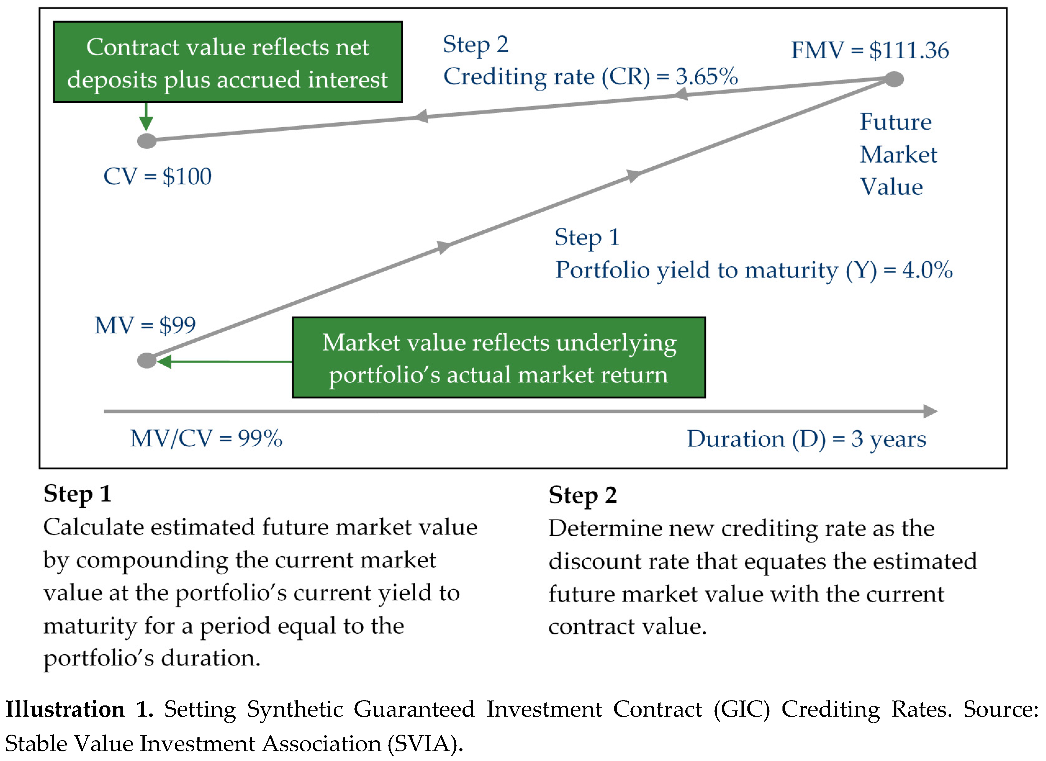
While this or a similar formula may serve as a starting point for a number of providers, ultimately (unless contractually specified otherwise) the crediting rates are determined by the provider itself, sometimes through committee decisions, and announced at or before the start of an ensuing crediting rate time interval. Furthermore, the crediting rates are set with competition in mind and a host of other economic factors. Investors are able to withdraw and redeploy their funds if they are dissatisfied with the pre-announced crediting rate, subject to the aforementioned restrictions.
4. Performance Measurement
In this study, we will measure the performance of SV funds vis-à-vis money market instruments,12 intermediate-term government bonds, long-term government bonds, corporate bonds, and small and large stocks using three methods of analysis: mean-variance analysis, stochastic dominance analysis, and enhanced multiperiod utility analysis. Each method has its advantages and drawbacks, but together we get a fairly clear picture of how well SV funds have performed. We conduct our analyses over the 27-year period beginning in 1989 when separate account GICs became an important component in the stable value market and, as a robustness test, over the extended 43-year period starting in 1973 that was dominated early by general account GICs.
We begin with a mean-variance analysis, more because of its simplicity and ubiquitous use in practice than its theoretical properties.13 Strictly speaking, the validity of this approach hinges upon whether investors consider variance to be an adequate measure of investment risk. In other words, investor preferences must be satisfactorily modeled using quadratic utility.
Beginning as early as 1967, Arditti (1967) determined that investors considered measures of downside risk beyond variance, and countless additional studies along similar lines have continued until now to demonstrate that variance is an inadequate measure of either security or portfolio risk.14 However, if the distribution of market returns can be fully described by its first two moments, then restricting one’s performance analysis to a mean-variance analysis can be justified, even if investors would otherwise be concerned about higher (and non-existent) moments of the return distribution. However, all tests with which we are familiar demonstrate that return distributions for stocks, bonds, and money market instruments cannot adequately be characterized by their means and variances, nor does modified Brownian motion fully capture the movement in these asset returns.
Accordingly, we next measure investment performance using stochastic dominance analysis. Introduced by Hanoch and Levy (1969) and by Hadar and Russell (1969) to remedy certain shortcomings of mean-variance analysis, stochastic dominance approaches have the clear advantage of taking into account all moments and other characteristics of the return distributions, and providing investment dominance analyses that do not depend upon knowing the exact shapes of investor preference functions. This has another distinct advantage over the mean-variance approach, which cannot be valid for various horizons simultaneously because it relies on log-normally distributed returns, and which if valid (under certain conditions) for single-period returns is not valid for multiperiod returns. By contrast, the stochastic dominance approach remains valid because it is distribution-free. The important additional virtues and limitations of this approach are discussed at length in the authoritative treatise by Levy (2006). While some of the limitations have been overcome by a plethora of research, dating from the 1970s to the present, there remain two:
- Stochastic dominance methods do not provide guidance into the construction of a portfolio from various individual securities.
- Stochastic dominance methods do not provide an equilibrium price for securities.
Our third approach is an indirect approach to performance measurement, based on the discrete-time multiperiod investment theory of Mossin (1968), Hakansson (1971, 1974), Leland (1972), Ross (1974), and Huberman and Ross (1983). Sometimes dubbed Turnpike Portfolio Theory, it remedies certain failings of mean-variance analysis as well as the limitations of stochastic dominance analysis at the high cost of specifying the form of the intertemporal preference function. To mitigate this high cost, in part, we will conduct our analysis across a wide range of risk aversion levels. Grauer and Hakansson (1982, 1985, 1986, 1987, 1993, 1995) and others, applied this theory to the asset allocation problem with some success, where an empirical probability assessment approach was used to implement a set of investment strategies. We will not rehearse the details of the methodology here, as they are well documented in Grauer and Hakansson (1986). The approach is indirect in the sense that we will determine whether, based on past asset return patterns and a range of current expectations, SV assets would enter the optimal portfolio in any significant way.
5. Data
The data of our primary focus are quarterly asset returns for the period Q4-1988 (shortly after the inception of stable value funds) through Q4-2015. We also include earlier data in Section 7 (Robustness Analysis), going back to Q2-1973, using the wrapped Lehman Intermediate Government/Credit Bond Yield series as a proxy for the return on traditional GICs, the precursors of SV funds. In addition to stable value (SV) funds, we consider six other asset classes, represented by large company stocks (LS), small company stocks (SS), long-term corporate bonds (LTCB), long-term government bonds (LTGB), intermediate term-government bonds (ITGB), and money market (MM). We describe each data series next.
Ibbotson’s stocks, bonds, bills, and inflation (SBBI) data are used for the following asset classes: LS (total return on the S&P 500), SS (the lowest 5% market cap in NYSE/AMEX/NASDAQ, comprising approximately 1700 stocks), LTCB (Citigroup Long-Term High Grade Corporate Bond Index, with an approximate maturity of 20 years), LTGB (each year, a newly issued government bond with approximate maturity of 20 years is used to calculate total return), and ITGB (each year, a newly issued government bond with approximate maturity of 5 years is used to calculate total return).
Money market returns are represented by the return on the Bank of America-Merrill Lynch US 3-Month Treasury bill Index (formerly the Lehman US Treasury Bellwether 3-Month Index). In Section 6.3, Intertemporal Optimization Analysis, where expected money market returns are an input to the optimization model, we use the yield series on 3-month Treasury bills, obtained from the Federal Reserve’s H15 database.
For SV funds, Q4-1988–Q4-2015, we use total net quarterly returns on various SV fund families managed by members of the Stable Value Investment Association (SVIA 2017). From the stable value data, we produce a composite index of stable value returns, including comingled funds, externally managed separate accounts, internally managed separate accounts, and life insurance general account stable value.15 As indicated above, when extending our analysis back to the second quarter of 1973, we use the wrapped Lehman Intermediate Government/Credit Bond Yield series as a proxy for the return on traditional GICs during the period Q2-1973–Q3-1988.
Although we have SV data for the four quarters of 2016, Morningstar stopped reporting the main SBBI series as of the end of 2015. It is mainly for this reason that our data end with the fourth quarter of 2015.
We note that except for small stocks and SV funds, reported returns are gross returns and need to be adjusted for management fees and transaction costs to be comparable to returns on small stocks and SV investments. We do this by subtracting average fees and expenses reported by the Investment Company Institute (ICI) for stock, bond and money market funds over the period of our analysis from the corresponding large stocks, bond or money market returns.16,17 Figure 1 below shows the evolution of mutual fund fees and expenses over the period of our analysis.
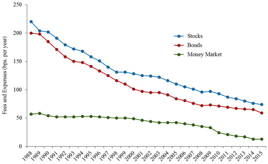
Figure 1.
Annual Fees and Expenses for Stock, Bond, and Money Market Funds.
Using these data as well as asset values for each fund complex, we construct an equal-weighted average return series. Figure 2 plots this series together with net quarterly return series for the intermediate-term government bond fund and money market fund series.18
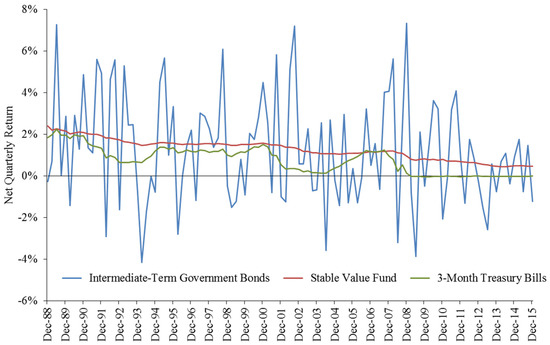
Figure 2.
Net Quarterly Returns—Stable Value Compared to intermediate term-government bonds (ITGB) and money market (MM).
Table 1 below presents summary statistics for the seven asset classes we study. It shows that over the period Q4-1988 through Q4-2015, SV investments have had, on average, a higher net quarterly return and a lower return volatility than either money market or intermediate-term government funds. As expected, when compared to stocks or long-term bonds, SV funds have exhibited both lower average returns and volatility. These facts lie behind the results that we present in the next section.

Table 1.
Summary Statistics—Net Quarterly Returns, Q4-1988–Q4-2015.
6. Results
6.1 Mean-Variance Analysis
As indicated earlier, mean-variance analysis provides a characterization of the trade-off between risk and return that is neither supported by the statistical properties of the return data, nor by the theoretical logic of risk aversion. Despite these shortcomings, the mean-variance approach provides useful insights into the ability of SV investments to dominate other asset classes.
In this section, we present evidence supporting the conclusion that, even as stand-alone investment, SV funds have been superior in the mean-variance sense to money market and intermediate-term government bond funds. We caution, however, that there are other important aspects of performance, discussed later, which are not captured by mean-variance analysis, so one should not jump to conclusions about the dominance of SV funds over these other asset classes based solely on mean-variance analysis. We also show, based solely on historical returns, that when included in optimal mean-variance portfolios, SV funds contribute significantly to the portfolio, to the exclusion of money market and intermediate-term government bonds, long-term corporate bonds and even large stocks. In other words, optimal mean-variance portfolios contain mostly SV funds, long-term government bonds and small stocks in proportions that naturally vary with the expected return (or, alternatively, the expected volatility) of the optimal portfolio. We anticipate that in the future, allocations toward long-term government bonds would be less, given that their inclusion in optimal portfolios to date was augmented significantly by a protracted period of capital gains stemming from declining Treasury yields.
When discussing summary statistics for our net quarterly return data in Table 1, we observed that, over the period of our study from October 1988 through December 2015, SV returns exhibited both a higher mean and lower volatility than either money market or intermediate-term government bond returns. This feature can be seen in Figure 3 below, where we plot two efficient frontiers, one including all seven asset classes in our study and one that excludes SV funds.
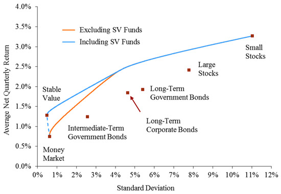
Figure 3.
Efficient Frontiers for Alternative Asset Classes (Q4-1988–Q4-2015).
It is interesting to note the potentially large scope for improvement that inclusion of SV investments brings to an optimal mean-variance portfolio across about half of the expected return range. As revealing as Figure 3 is, it does not show the full extent to which SV investments contribute to an optimal portfolio since it says nothing about the relative allocations of wealth among SV funds and other investments at different points along the efficient frontier. Table 2 reports these optimal weights (again based solely on historical returns) for selected expected quarterly returns ranging from 1.28%, the historical average net return for SV funds, to 3.27%, the historical small stocks net return.
Table 2.
Optimal Portfolio Weights for Mean-Variance Efficient Portfolios Including SV (Q4-1988–Q4-2015).
We observe that no optimal mean-variance portfolio along the efficient frontier points shown in Table 2 includes money market instruments and intermediate-term bonds but includes only very small allocations toward large US stocks and minuscule allocations toward long-term corporate bonds. We also observe that SV funds predominate in the lower portion of the expected return range, where one would conventionally anticipate seeing money market and intermediate-term bond investments.
Table 3 repeats the optimal portfolio analysis but where SV is not included as an available asset class. We observe that money market instruments and intermediate-term bonds now enter the optimal portfolios at various levels of portfolio risk, along with small and large stocks and long-term government bonds. We also observe that large US stocks and long-term corporate bonds modestly increase their presence among efficient frontier portfolios.
Table 3.
Optimal Portfolio Weights for Mean-Variance Efficient Portfolios Excluding SV (Q4-1988–Q4-2015).
Continuing in the spirit of mean-variance analysis, we turn to the Sharpe ratio so commonly used in asset al.location and performance measurement.19 The Sharpe ratio measures excess return per unit of risk according to the formula:
where R is the asset return, Rf is the return on the risk-free rate of return, and E[R − Rf] is the expected value of the excess of the asset return over the risk-free rate. This ratio is used as a measure of how well an investor is compensated per unit of risk taken. Higher ratios denote greater return for the same level of risk.
We also use the Sortino ratio to focus more on the downside risk.20 The Sortino ratio is based on the Sharpe ratio, but penalizes for only those returns that fall below the target return, which in our case will be the average riskless rate of return over the period of analysis. The ratio gives the actual rate of return in excess of the risk-free (target) rate per unit of downside risk (i.e., target semi-deviation or average of squared deviations below the target rate), and is as calculated below:
The Sharpe and Sortino ratios for quarterly net return data are reported in Table 4.
Table 4.
Sharpe and Sortino Ratios (Quarterly Data, Q4-1988–Q4-2015).
We note that the Sharpe ratio values for the non-SV asset classes are mostly clustered together, but that for SV the ratio is more than seven times greater than the highest of the other asset classes. This pattern is even more pronounced for the Sortino ratio. The extremely high Sortino ratio assigned to SV funds, relative to those assigned to other asset classes, results from the fact that throughout the entire 109 quarter period under consideration, the risk-free rate exceeded the SV credited rate only for four quarters (in Q3-2006 and Q1–Q3-2007) and by small amounts. Hence, there were only a few, small observations that factored into the denominator.
What is most noteworthy about these performance ratios is how much higher they are for SV funds than for the other asset classes. Although our calculations are based primarily on quarterly data, we also provide the analogous ratios based on annual returns in Table 5. Again, we observe very large Sharpe and Sortino ratios for SV funds relative to other investment classes.
Table 5.
Sharpe and Sortino Ratios (Annual Data, 1989–2015).
What we can say from this ratio analysis is that the structure of SV returns is very different from that of other asset classes, and that its structure does not lend itself well to traditional mean-variance metrics for comparison. Moreover, these mean-variance findings are derived from returns that, for most investment classes, are generally not normally distributed, as evidenced by the bottom row of Table 1 displayed earlier. Accordingly, we now turn to present alternative and more powerful analyses that buttress the implications of our mean-variance analyses.
6.2. Stochastic Dominance Analysis
We next discuss the ability of SV funds to dominate alternative asset classes in the sense of stochastic dominance (SD) which, as we indicated earlier, provides dominance criteria under very general conditions with respect to an investor’s attitudes toward risk and considers higher moments of the asset return distributions.
First-degree stochastic dominance (FSD) imposes only one preference restriction—investors prefer more wealth to less wealth. In addition to this requirement, second-degree dominance (SSD) requires investors to be risk averse, i.e., to dislike a drop in wealth more than they like a wealth increase of the same magnitude. The development of third-degree stochastic dominance (TSD) was motivated by a long observed preference among investors for positively skewed returns. A subset of the class of investors that prefer returns exhibiting third-degree stochastic dominance is the important group whose preferences are characterized by decreasing absolute risk aversion (DARA). Such investors are willing to pay less for insuring against a given sized risk, on average, as they accumulate greater wealth, which appears to accord with observed behavior toward risk. Fourth-degree stochastic dominance (4SD) was developed to capture investors’ aversion toward kurtosis, where returns are characterized by peaked distributions and fat tails, such that losses can be extreme. Of course, kurtosis can favor investors who have asymmetric claims toward returns, such as investors in call options, but for investors who have equal claims to both tails of a distribution, the fatter tails cause a disproportionate loss in utility.21
Table 6 presents the SD results among the seven asset classes in our study, based solely on historical returns. Only the SV historical returns distribution dominated two asset classes in the stochastic dominance sense up to the fourth degree; none of the other asset classes dominates any other class of funds, including SV funds.
Table 6.
Stochastic Dominance among Alternative Asset Classes. Net Quarterly Returns Q4-1988–Q4-2015.
Turning to SV funds, they stochastically dominated money market investments by the first-degree and, as a corollary, by any higher degree as well. Consequently, based on historical returns alone, any investor who preferred more wealth to less wealth should have avoided investing in money market funds when SV funds were available, irrespective of risk preferences. Of course, historical returns alone cannot establish dominance going forward, and expectations of future returns may well depend on factors not included by historical conditions.
Although SV funds failed to stochastically dominate intermediate-term government bonds by the first degree, they dominated by the second and higher degrees.
The results in this sub-section are remarkable. Not surprisingly, there is no stochastic dominance of any one traditional class over another; indeed dominance is rarely encountered in empirical studies of asset classes. Accordingly, it was surprising to find that SV investments dominated two of the major traditional investment classes.
6.3. Intertemporal Optimization Analysis
In this section, we look at the potential gains of including stable value funds in an investor’s portfolio when risk-aversion is explicitly taken into consideration and the investor maximizes expected utility of wealth in a dynamic setting. At the cost of making additional assumptions about an investor’s attitudes toward risk, this analysis provides additional insights into the role that stable value funds could play in portfolio design.
Our theoretical framework follows the intertemporal investment model of Grauer and Hakansson (1982, 1985, 1986, 1987, 1993, 1995), considering an investor who, at the beginning of each period, allocates wealth among various investment alternatives so as to maximize expected utility of wealth. The investment alternatives we consider are the same as in our previous analysis, with investment horizon assumed to be a quarter. Therefore, the return data we use are net quarterly returns for the period Q1-1989 through Q4-2015.
In Grauer and Hakansson’s model (esp. 1982), new information about the distribution of assets is incorporated prior to each quarterly optimization and the utility-maximizing portfolio for the quarter is derived. More specifically, at the beginning of the optimization quarter t, the investor determines portfolio weights, , that maximize expected utility of wealth,
subject to for all i and . E[·] is the expectations operator, wit is the fraction of wealth allocated to investment i in period t, rit is the return on investment i over quarter t, and a ≤ 1 is a risk parameter.22 The function U(·) is the constant relative risk aversion (CRRA) utility function with coefficient of relative risk aversion given by
In Grauer and Hakansson (1982), the empirical distribution of returns is used to approximate the unknown joint distribution of returns. This approach is referred to as the “simple probability assessment approach.” The authors use quarterly data over the 40 quarters (or ten years using annual data) prior to the optimization quarter (year) in order to compare the performance of the portfolio consisting of the series of optimal quarterly (or annual) portfolios over the 1936–1978 period (with data for the 1926–1978 period) with the performance over the same period of the individual asset classes they consider.
We examine data for 80 quarters prior to each optimization quarter.23 Given the historical sample we employ, this means that our first optimization quarter is Q1-1993 and the last one is Q4-2015. Over these 92 quarters, a representative investor determines the optimal portfolio for each quarter, each time using the empirical distribution of returns from the immediately preceding 80 quarters to maximize expected utility as described above. At the end of the 92 quarter period, the (geometric) average portfolio return and the standard deviation of returns are calculated for two portfolios, one that excludes stable value funds and another that includes them.
One empirical problem for this analysis is that bond yields have been decreasing steadily over the period examined and empirical past return averages for mostly any given quarter will therefore tend to overestimate the population expected future returns. For this reason, we modify Grauer and Hakansson’s simple probability assessment approach by estimating bond returns at the start of each optimization quarter with their respective yields (on a quarterly basis). We do this for long-term corporate and government bonds and for intermediate-term government bonds. More specifically, for each of these bond series in each optimization quarter, the quarterly deviations from their respective means (over the previous 80 quarters) are added to the corresponding current bond yields (expressed as a quarterly return). In this way, we preserve the joint co-movements of all asset classes subject to uncertain returns over each optimization quarter.24
We note that at the start of each optimization quarter, the expected return on the money-market and stable value funds is non-random. As indicated in Section 5 above, we use the yield on 3-month Treasury bills to approximate the expected returns on the money market fund and the promised crediting rate as the return on the stable value fund.
In a second piece of analysis, we focus on the last four quarters of 2015 and construct scenarios for the expected return on large and small stock returns based on a range of assumed respective large and small equity premiums over money market yields. The equity premiums chosen reflect those encompassed by survey data given by Fernández et al. (2015, 2017). This allows us to simulate the performance of SV funds under various stock return scenarios during a period where crediting rates have been lowest due to the secular decline in interest rates.
6.4. Optimal Portfolio Returns Q1-1993–Q4-2015
In this section, the question of interest is what would be the (geometric) average quarterly return and volatility for a portfolio that is optimally rebalanced every quarter between 1993 and 2015, according to the rules set out above. We provide answers to this question for selected values of the risk aversion coefficient a in expression (6) above and for portfolios excluding and including stable value. Table 7 shows mean quarterly returns and standard deviations for each of these cases and Figure 4 illustrates the same results in the mean-standard deviation plane. The risk aversion values of a range from +1 to −75, the same range employed by Grauer and Hakansson in their seminal papers. Also, research by Malloy et al. (2009) supports high degrees of risk aversion.
Table 7.
Geometric Quarterly Means and Standard Deviations for Optimal Portfolios, Q1-1993 through Q4-2015.
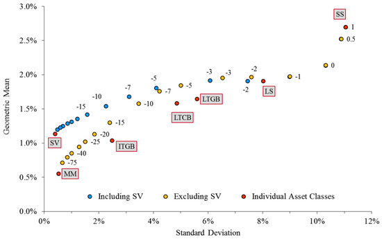
Figure 4.
Optimal Portfolios for Selected Risk Aversion Parameters, Excluding and Including Stable Value Assets.
The top panel in Table 7 reports the geometric mean returns and standard deviations of the various asset classes involved. These can be interpreted as portfolios that hold only one security throughout the period 1993–2015 and so can be compared to the optimizing portfolios in the lower panel of Table 7, which shows the optimizing results across the whole spectrum of risk aversion levels.
In Figure 4, we plot the optimal risk–return pairs in Table 7. More specifically, we plot optimal portfolios for selected risk-aversion parameters when SV returns are included and optimal portfolios when SV returns are excluded. We also plot with the geometric mean returns and standard deviations, over the same period, Q1-1993 through Q4-2015, for the asset classes we consider.
The case where the risk parameter a equals 1 is that of linear utility and risk is of no concern to the risk-neutral investor. Since in our sample, average returns for all quarters in 1993–2015 (based on the previous 80 quarters of data) are highest for small stocks (SS), the sequence of optimal portfolios for such a risk-neutral investor implies holding small stocks throughout the period, excluding any other asset class, and obtaining a geometric average quarterly return of 2.70% and a quarterly standard deviation of 11.04%.
The case where the risk parameter a equals 0 is that of logarithmic utility and while it exhibits some degree of risk aversion it is not enough to induce an investor to hold lower-yielding assets.
The inclusion of stable value assets in the mix of asset classes begins to make a difference with risk parameter of a = −2 (corresponding to a coefficient of relative risk aversion of ρ = 1 − a = 3). In particular, we observe that the inclusion of stable value reduces the portfolio’s average standard deviation for risk parameter less than or equal to −2 and increases the geometric mean return for values of the risk parameter less than or equal to −15. For this case, the quarterly average portfolio return is 1.42% and the average standard deviation is 1.57% when stable value is included, compared to 1.30% and 2.40% when excluded.
In order to directly observe the composition of the optimal portfolios quarter by quarter, we plot the optimal quarterly allocations, excluding and including stable value (SV) assets in Figure 5, Figure 6, Figure 7, Figure 8, Figure 9, Figure 10, Figure 11 and Figure 12 for selected values of the risk parameter.
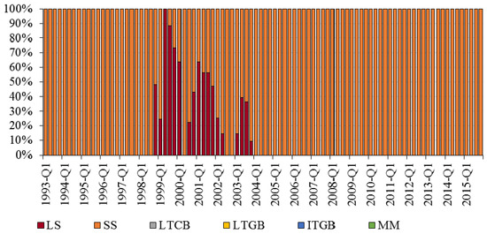
Figure 5.
Optimal Allocations by Quarter for Risk Parameter a = 0 (Excluding SV).
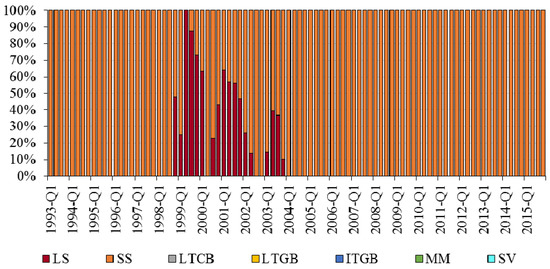
Figure 6.
Optimal Allocations by Quarter for Risk Parameter a = 0 (Including SV).
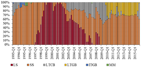
Figure 7.
Optimal Allocations by Quarter for Risk Parameter a = −2 (Excluding SV).
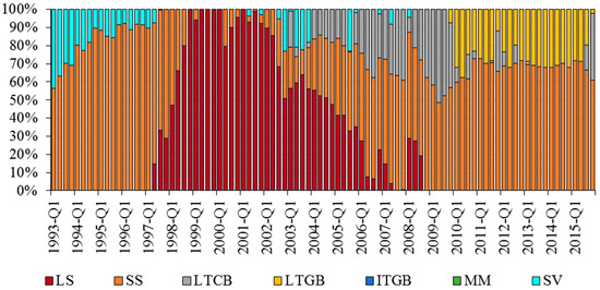
Figure 8.
Optimal Allocations by Quarter for Risk Parameter a = −2 (Including SV).
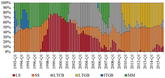
Figure 9.
Optimal Allocations by Quarter for Risk Parameter a = −5 (Excluding SV).
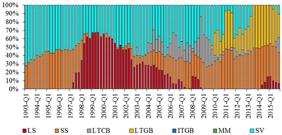
Figure 10.
Optimal Allocations by Quarter for Risk Parameter a = −5 (Including SV).
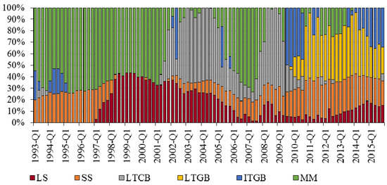
Figure 11.
Optimal Allocations by Quarter for Risk Parameter a = −10 (Excluding SV).
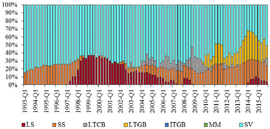
Figure 12.
Optimal Allocations by Quarter for Risk Parameter a = −10 (Including SV).
In Figure 5 and Figure 6 we observe that for logarithmic utility only large and small stocks are included. Indeed, except for a few quarters, concentrated in the period 1999–2003, optimal portfolios consist of small stocks alone. Accordingly, the quarterly geometric mean return and the standard deviation in this case over the period 1993–2015 are, respectively, 2.14% and 10.31%.
Besides these two cases where the degree of risk aversion is nonexistent or low, relevant questions are, therefore, at what level of risk aversion do lower-yielding assets begin to play a significant role in optimal portfolios and, specifically for our inquiry, at what level of risk aversion do stable value investments begin to play a significant role in optimal portfolios and what other asset classes do they replace when included. Figure 7, Figure 8, Figure 9, Figure 10, Figure 11 and Figure 12 below provide an answer to these questions.
For risk aversion parameter a = −2 and excluding stable value investments, optimal portfolios include more small stocks and moderate amounts of long-term corporate and government bonds, with a small amount of intermediate-term government bonds and money market funds around 1995 and 1996 (Figure 7). When stable value funds are included (Figure 8), they entirely replace intermediate-term government bonds and money market funds. Interestingly, stable value funds also partially replace small stocks in the 1993–1997 sub-period and some long-term corporate bonds around 1993–1994 and 2003–2004.
For moderate and higher levels of risk aversion, that is values of a around −5 or −10, the preponderance of stable value funds becomes very clear, entirely crowding out money market investments and intermediate-term government bonds, and significantly replacing long-term corporate and government bonds. Figure 9, Figure 10, Figure 11 and Figure 12 illustrate these two cases.
As can be seen earlier in Table 7, at levels of the risk parameter a equal to −5 or −10, the geometric average quarterly return including stable value funds, 1.80% and 1.54%, respectively, is slightly lower than the corresponding averages excluding stable values, 1.85% and 1.58%, respectively, but the standard deviations are much smaller, at 4.07% compared to 5.00% for a = −5 and 2.24% compared to 3.45% for a = −10. For values of the risk parameter smaller than −10, that is, as risk aversion becomes significant, Table 7 shows that including stable value in the investors’ options both increases average returns and reduces the portfolio’s standard deviation.
6.5. Sensitivity to Expected Stock Returns
In the previous analysis, we have used historical returns for large and small US stocks in modeling the joint distribution of quarterly returns. There is, however, an ongoing discussion about what the equity premium may be in the future (Fernández et al. 2015, 2017), suggesting that past historical equity premiums may not be an accurate estimate of future equity premiums. This observation echoed that presaged by Siegel (2005) some ten years earlier.
In this section, we conduct a scenario analysis in which we use three levels of the equity premium, 3%, 5%, and 7% per year, over the money market yield for each optimization quarter. Therefore, the expected return for a given optimization quarter in a given scenario is constructed as the promised 3-month yield plus the scenario’s large stock equity premium (3%, 5%, or 7%). For small stocks, we add the historical average return spread between small and large stocks over the 80 quarters of data used for each optimizing quarter to the corresponding expected large stock return just described.
As in the previous section, we preserve the co-movement of the asset classes considered by adding the quarterly deviations of historical returns from their respective sample means to their current modeled expected returns for large and small stocks, long-term government and corporate bonds, and intermediate-term government bonds.
Figure 13, Figure 14, Figure 15, Figure 16, Figure 17 and Figure 18 show the asset weights of optimal portfolios for the three large stock equity premium scenarios considered, at selected risk parameters and varying assumed equity premia for the four quarters of 2015.25 Interestingly, these figures will show that long-term corporate bonds play a much larger role in optimized portfolios than they did in our earlier mean-variance analysis, whether or not stable value is considered. This larger role stems from two sources. First, the intertemporal optimization analysis takes into account all of the statistical moments of the distribution of returns, and not only its mean and variance. Thus, the risk measure includes more information and is more robust to variations in risk tolerance. Second, the larger role of long-term corporates is evident primarily during the 2002–2010 period, but not particularly noticeable outside of that range of years, whereas the mean-variance analysis was based on the entire period from 1989–2015. Moreover, beginning in 2008, Treasury yields plummeted to almost record lows and volatility increased, but high-grade corporate bond yields were comparatively stable, as were their prices. Thus, the risk–return dynamics were altered between these two classes of fixed income.
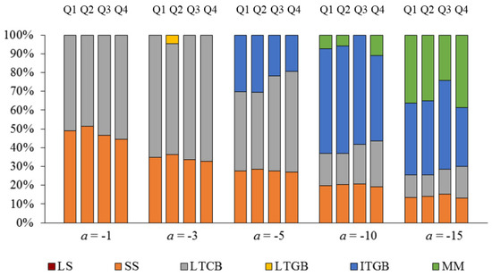
Figure 13.
2015 Optimal Portfolios (LS Equity Premium = 3%)—Excluding SV.
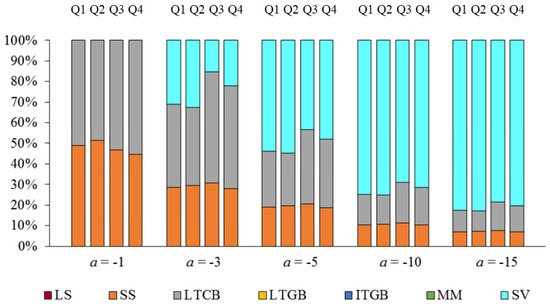
Figure 14.
2015 Optimal Portfolios (LS Equity Premium = 3%)—Including SV.
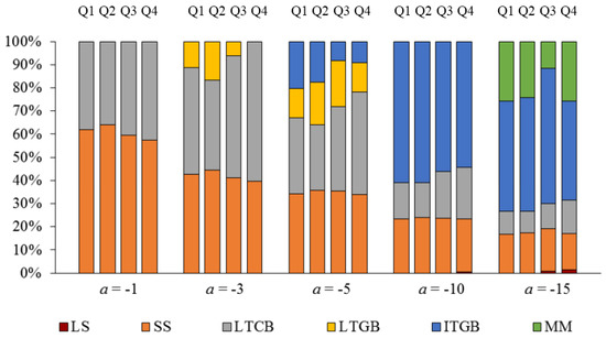
Figure 15.
2015 Optimal Portfolios (LS Equity Premium = 5%)—Excluding SV.
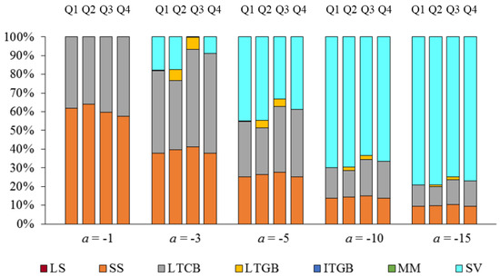
Figure 16.
2015 Optimal Portfolios (LS Equity Premium = 5%)—Including SV.
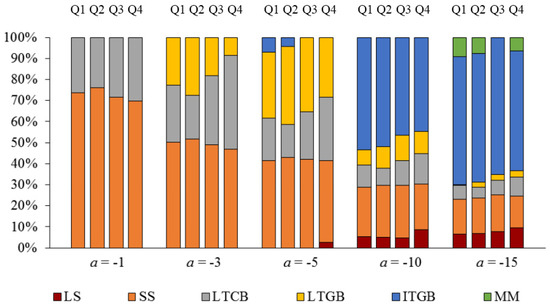
Figure 17.
2015 Optimal Portfolios (LS Equity Premium = 7%)—Excluding SV.
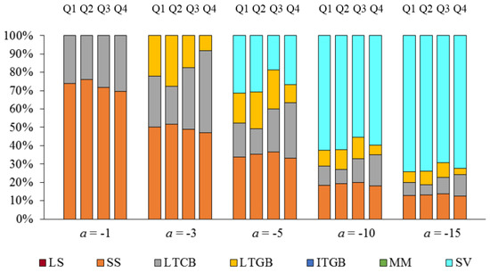
Figure 18.
2015 Optimal Portfolios (LS Equity Premium = 7%)—Including SV.
The general pattern that can be observed in Figure 13, Figure 14, Figure 15, Figure 16, Figure 17 and Figure 18 is that stable value entirely replaces money market and intermediate-term government bonds. Also, beginning at intermediate levels of the risk parameter such as a = −3 and a = −5, stable value partially crowds out long-term corporate and government bonds.
7. Robustness Analysis
While important, the implications of our three-fold analysis should not be regarded as dispositive. It should be recalled that over the 27-year period of the first phase of our analysis, which began with the inception of modern SV funds in 1989, interest rates exhibited a general decline to half their initial level, albeit with occasional and protracted periods of rising interest rates interspersed. Such a period of decline would tend to favor longer duration fixed income investments, including stable value, over money market funds. We sought to remedy this by including the precursors of SV funds—traditional GICs—to see how they fared during the period of rapidly rising interest rates that characterized the late 1970s and early 1980s.26
7.1. Period Q2-1973–Q3-1988
We first report results for the earlier period Q2-1973–Q3-1988 and then present results for the combined period Q2-1973–Q4-2015. Table 8 reports summary statistics for the extended period Q2-1973 through Q3-1988.
Table 8.
Summary Statistics—Net Quarterly Returns, Q2-1973–Q3-1988.
Comparing Table 1 and Table 8, we observe that average returns for a particular asset class vary considerably, especially for small stocks, money market, intermediate-term governments, and SV returns. Small stocks have an average net quarterly return of 5.22% for the earlier period, compared with 3.27% for the period Q4-1988 through 2015. This difference is essentially due to the better performance of small stocks over the period 1973–1988. The 128 basis points jump in money market quarterly average return for the earlier period is due to the higher yields on debt instruments observed during the late seventies and early eighties. This is also the reason that the SV quarterly average return increased by 73 basis points to 2.01% for this period compared to the average of 1.28% over the period Q4-1988–2015. Returns on intermediate-term governments averaged 59 basis points higher than the later period.
7.2. Mean-Variance Analysis
The differences we observe in mean returns across the two sample periods considered are reflected in the efficient frontier corresponding to the Q2-1973 through Q4-1988 data, shown in Figure 19, contrasted with Figure 3 earlier.
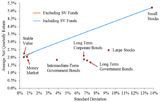
Figure 19.
Efficient Frontiers for Alternative Asset Classes (Q2-1973–Q4-1988).
We observe a steeper but much less curved efficient frontier for the early sample period. The higher steepness is clearly the result of the higher small stocks average return compared to its corresponding value for the Q4-1988–Q4-2015 sample period; and the smaller curvature is due mostly to the way asset correlations changed from the earlier to the latter sample periods.27
Table 9 reports these efficient portfolios for selected points along the efficient frontier. We observe that the composition of the efficient portfolios reported earlier in Table 2 changes in some respects when the earlier sample is considered here, but it also remains the same in other respects. Table 9 (covering the earlier period) shows that large stocks, long-term corporate and government bonds, and intermediate-term bonds are completely excluded from the efficient frontier whereas in the Q4-1988–Q4-2015 sample reported in Table 2, large stocks had at least a slight participation and in one case (at the lowest risk level) long-term corporates even entered the efficient frontier marginally. We also observe that the weights of money market funds, which were entirely excluded in the later period, are now substantial across most portfolio risk levels. In most cases, the weights even exceed those for stable value shown in Table 2.
Table 9.
Optimal Weights for Mean-Variance Efficient Portfolios Including SV (Q2-1973–Q3-1988).
The two most important differences with Table 2 were that the weight of long-term government bonds is now much decreased (from an average holding of 30% to 0%) across all efficient portfolios and that the weight of small stocks is decreased markedly across the portfolio standard deviation ranges that overlap both tables. The principal reason for the higher weights on long-term governments in the later period was the capital gains boost on their returns as market yields generally declined over a prolonged period. The reason that small stocks had lower weights in the earlier period when compared to portfolio weights across similar portfolio risk levels in the later period was that quarterly money market returns were so high during this period (2.03% on average, compared to 0.75% since Q4-1988) and had a much smaller volatility than small stocks, as shown in Table 1 and Table 8.
Table 10 repeats the optimal portfolio analysis but where SV is not included as an available asset class. We observe that money market instruments enter the optimal portfolios at all levels of portfolio risk except the highest level, along with small stocks. No long-term or intermediate bonds are included at all, and large stocks enter only once at the very lowest risk level. Note that, unlike the results of the more recent period shown in Table 3, intermediate-term bonds no longer enter the optimal portfolios at any levels of portfolio risk even though there is no SV to dominate them. Finally, in comparing the first two columns of Table 9 with the corresponding columns in Table 10, we see by using simple interpolation that for only the lowest few levels of expected returns in a portfolio precluded from SV assets, the risk is higher than for the case when SV is included.
Table 10.
Optimal Weights for Mean-Variance Efficient Portfolios Excluding SV (Q2-1973–Q3-1988).
7.3. Sharpe and Sortino Ratios
Comparable Sharpe and Sortino ratios are calculated for the earlier sample and reported in Table 11 and Table 12 below.
Table 11.
Sharpe and Sortino Ratios (Quarterly Data, Q2-1973–Q3-1988).
Table 12.
Sharpe and Sortino Ratios (Annual Data, 1974–1988).
We note that unlike the later period (Q4-1988 through Q4-2015), during which the money market rate exceeded the SV rate in four out of the 109 quarters in the period (about 3.7% of the time), the earlier period of 62 quarters contained 26 quarters (about 41.9% of the time) during which money market yields exceeded the corresponding SV rates. It is therefore interesting to observe that extending the sample to include a period of significantly higher interest rates reduced the mean-variance-based performance of SV funds relative to its dominating position in the later period, although it still entered optimal portfolios at low-risk levels.28 The Sharpe and Sortino ratios exhibited by SV funds were again superior to other fixed income categories (for annual data), but lower than their equity counterparts, as shown in Table 11 and Table 12.
7.4. Stochastic Dominance
Turning to the issue of stochastic dominance, we find that SV no longer dominates money market investments, as was the case for the 1989 to 2015 period. Neither do money market investments dominate SV. Yet both SV and money market investments dominate corporate and government long-term bonds as well as intermediate-term governments for all risk-averse investors (2nd degree and higher). We also note that that long-term corporates dominate long-term governments at the 3rd degree and that intermediate-term governments dominate long-term governments at the 2nd degree, yet intermediate governments are already dominated by SV and money markets, so it is not particularly impressive. Also, this would be expected to occur in an era of rising interest rates, where long duration bonds suffer larger capital losses than their shorter-term counterparts.
The stochastic dominance relationships obtained in Table 13 are remarkable in the sense that they are strikingly different from those that were obtained in the main period of our study Q4-1988–Q4-2015.
Table 13.
Stochastic Dominance among Alternative Asset Classes. Net Quarterly Returns Q2-1973–Q3-1988.
7.5. Full Sample Q2-1973–Q4-2015
In closing out our robustness analysis, we reexamine SV performance over the entire extended period from 1973 to 2015. The relevant tables and charts are provided below. The analysis shows that over the extended period, there is only one asset class that dominates any of the others, and that is stable value. It again shows that no asset class dominates stable value, which was also true over both the early and later sub-periods. As can be expected, mean-variance, Sharpe and Sortino ratios, and stochastic dominance analyses over the full sample period will produce results that are in between the two sets of results discussed for the earlier and later periods. It is nevertheless illustrative to see how far or close are the combined sample results from either of the two sets. Financial and economic conditions were very different between the two periods we have considered and if there is one financial feature that can be singled out from the rest it is the very different behavior of US short-term interest rates that we have observed.
Table 14, Table 15, Table 16, Table 17 and Table 18 and Figure 20 below summarize the data and results for the full sample period Q1-1973–Q4-2015.
Table 14.
Summary Statistics—Net Quarterly Returns, Q2-1973–Q4-2015.
Table 15.
Optimal Weights for Mean-Variance Efficient Portfolios Including SV (Q2-1973–Q4-2015).
Table 16.
Optimal Weights for Mean-Variance Efficient Portfolios Excluding SV (Q2-1973–Q4-2015).
Table 17.
Sharpe and Sortino Ratios (Quarterly Data, Q2-1973–Q4-2015).
Table 18.
Sharpe and Sortino Ratios (Annual Data, 1974–2015).
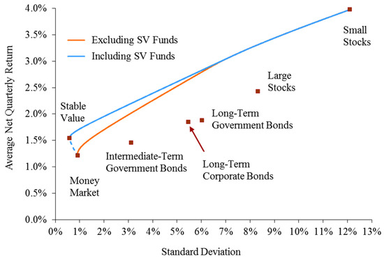
Figure 20.
Efficient Frontiers for Alternative Asset Classes (Q2-1973–Q4-2015).
7.6. Mean-Variance Analysis
The differences we observe in mean returns across the two sample periods considered are reflected in the efficient frontier corresponding to the Q2-1973 through Q4-2015 data, shown in Figure 20, contrasted with Figure 3 earlier.
As was the case with the earlier period, we observe a steeper but less curved efficient frontier for the full sample period, compared to the Q4-1988–Q4-2015 period. The curvature is still significantly less than for the later period because over the full sample period the correlations between long-term and intermediate-term bond returns with small stock returns continue to be significantly higher that for the period Q2-1973–Q3-1988 alone.29
Table 15 reports these efficient portfolios for selected points along the efficient frontier. We observe that the composition of the efficient portfolios reported earlier in Table 2 changes in some respects when the extended sample is considered here, but it also remains the same in other respects. Table 15 (covering the extended period) shows that large stocks, long-term corporate bonds, intermediate-term bonds and money market assets are completely excluded from the efficient frontier whereas in the Q4-1988–Q4-2015 sample reported in Table 2, large stocks had at least a slight participation and in one case (at the lowest risk level) long-term corporates even entered the efficient frontier marginally. We also observe that the weights of SV funds are markedly larger than for the portfolios shown in Table 2.
Another important difference with Table 2 is that the weight of long-term government bonds is now much decreased (from an average holding of 30% to 20%) across all efficient portfolios and the weight of small stocks is correspondingly increased.
Table 16 repeats the optimal portfolio analysis but where SV is not included as an available asset class. We observe that money market instruments enter the optimal portfolios at various levels of portfolio risk, along with small stocks and long-term government bonds. However, unlike the results of the shorter period shown in Table 3, intermediate-term bonds no longer enter the optimal portfolios at any levels of portfolio risk even though there is no SV to dominate them. We also observe that large stocks and long-term corporates enter mean-variance-efficient portfolios only once, at the lowest expected return and standard deviation combination, when calibrations are based on the past 43 years of historical returns and correlations. Finally, in comparing the first two columns of Table 15 with the corresponding columns in Table 16, we see by using simple interpolation that for most given expected returns in a portfolio precluded from SV assets, the risk is higher than for the case when SV is included.
7.7. Sharpe and Sortino Ratios
Comparable Sharpe and Sortino ratios are calculated for the extended sample and reported in Table 17 and Table 18 below.
We note that unlike the shorter period (Q4-1989 through Q4-2015), during which the money market rate exceeded the SV rate in four out of the 109 quarters in the period (about 3.7% of the time), the extended period of 171 quarters contained 30 quarters (about 17.5% of the time) during which money market yields exceeded the corresponding SV rates. It is therefore interesting to observe that extending the sample to include a period of significantly higher interest rates does not adversely affect the relative performance of SV funds. Again, the Sharpe and Sortino ratios were spread across a relatively narrow range for the other asset classes, but the SV ratios soared far above the rest for both quarterly and annual data, as shown in Table 17 and Table 18.
7.8. Stochastic Dominance
Consistent with the stochastic dominance results discussed earlier in this section for the period Q2-1973–Q3-1988, we find that SV no longer dominates money market investments by the first degree, as was the case for the 1989 to 2015 period. This can be easily deduced from Table 14 above since the maximum quarterly money market return (3.93%) exceeds the maximum quarterly SV return (2.64%), thereby precluding the possibility of SV exhibiting complete FSD over money market returns. This lack of first-degree dominance is a consequence of the high interest rates observed in the late seventies and early eighties, compared to the smaller SV returns which behave like smoothed intermediate-term bond yields. However, over the extended period, SV returns continue to exhibit second-and higher-degree stochastic dominance over money market funds, as well as over intermediate-term government bonds. Other than this change, the stochastic dominance relationships among the asset classes in our study for the extended period are as shown in Table 6 above.
The analysis in this section shows that the relatively good performance of SV investments is robust (one is tempted to say stable) to the sample period considered in the sense that the extended period we use includes extreme interest rate movements in both directions as well as extreme stock return fluctuations.
8. The Value Proposition, Challenges and Future Prospects
The positive evidence thus far, which covers the entire period of existence for traditional and synthetic forms of stable value funds, is intriguing and raises two questions: (1) What has been the value proposition that allowed these returns to be achieved? And (2) should we expect this kind of performance over the future?
In essence, the theoretical principle behind stable value’s popularity is the clever “financial engineering” idea behind transforming an asset portfolio that generates total rates of return into a stable value product that offers the design of a smooth yield-like return, coupled with investor risk-aversion. So it is both risk and return repackaging that drive SV’s popularity. Notice that this dominance disappears when the risk–return profile, combined with low degrees of investor risk aversion, is more tilted towards return.
More specifically, the value proposition has two facets. On the asset side, some of the return above money market yields comes from investing at durations sufficiently long to capture the term premium that has been traditionally available in most markets. The funds also are able to take on a very small amount of credit and convexity risk and thereby gain some additional spread. They also sometimes invest in less liquid securities, structured notes and occasionally GICs, which provide higher spreads than the most liquid assets. The first factor helps explain why SV returns have generally outpaced money market yields, but does not explain why they also have outpaced intermediate-term government returns. For that, we must turn to the other three factors—credit risk, negative convexity, and lower liquidity.
On the liability side, the contribution to performance derives from behavioral finance factors. Stable value funds have contingent liquidity that the Financial Accounting Standards Board (FASB) and the Governmental Accounting Standards Board (GASB) define as “benefit responsive.” From the point of view of participants, SV has the same liquidity as money market funds. Banks, insurers or other financial institutions that issue the investment contracts take on the transfer/liquidity risk as well as the investment/market risk that everyone will not withdraw at the same time, since the underlying portfolio has to be less than contract value to cause the investment contract to make up the difference between market and contract value.
Stable value providers mitigate their risk largely by being astute at predicting and underwriting participant behavior. They know that the vast majority of participants, because of tax penalties, equity wash requirements that inhibit interest rate arbitrage, and simple investor inertia, tend to leave their money in stable value options for a fairly long time. Providers are willing, therefore, to guarantee a fixed rate for a traditional GIC and a minimum zero percent crediting rate each quarter for a synthetic GIC. Defined contribution participants in SV want mostly principal stability and do not need daily liquidity for all balances. This allows the wrap providers to offer their guarantees at a lower price than otherwise would be the case. Any disintermediation that has occurred prior to the recent financial crisis has been occasioned by a run-up in equity prices, and not associated with a rising interest rate environment. This means that the wrap providers historically have not suffered massive withdrawals when costly interest rate arbitrage typically occurs. Because defined contribution participants tend to care more about principal stability than daily liquidity for all balances, this allows fund managers to benefit from the steepness of the yield curve and seek credit and liquidity spreads. By contrast, money market funds must provide both principal stability and a lot more liquidity, which participants pay for in the form of a lower return.
To be able to maintain the attractiveness of their funds, SV fund managers will need to continue facing yield curves that generally have positive steepness. Historically, however, yield curves have flattened and even inverted at times, so SV providers need to be prepared for such eventualities by employing some combination of hedging, pricing margins, and reserve funds. High quality assets that offer attractive yields due to lower liquidity, negative convexity (which does little harm to stable yields), and adequate credit spreads must continue to be available at suitable prices. Furthermore, for SV managers to seek such yields will require that their funds continue to be offered only through vehicles such as defined contribution programs which cater to investors willing to be patient, while eschewing day traders and interest arbitragers. Stable value funds would probably not survive outside of that kind of protected environment. (We note that hedge funds often provide a different kind of “stickiness” with respect to exit and cash-out provisions.) In the past, stable value has incorporated relatively low management fees into its funds (averaging 60% of the fees charged by the average bond fund), which included a low wrap cost of around 4–8 b.p. During the Great Recession, wrap fees reached levels of 20–25 b.p. and higher, creating upward pressure on total fees subtracted from the returns offered to investors. However, as additional wrap providers entered and reentered the market, these fees have fallen somewhat. In any case, aggregate fees have remained low and this has contributed to SV’s continuing relatively good performance.
Since their inception in 1973, SV funds have undergone several severe tests. They survived the market fallout from the OPEC cartels, the severe stock market declines of 1973–1974, 2000–2002, the stock market crash of 1987, the interest rate spikes of the early 1980s, the liquidity and credit spread crisis of the late 1990s, the plummeting interest rates of the 21st century, economic booms and deep recessions, the terrorist challenges to financial markets in 2001, and countless other daunting circumstances. With few exceptions,30 they weathered the recent financial crisis of 2007–2009, even while the number of wrap providers dwindled briefly from 25 to less than a dozen, precipitating steep increases in wrap fees among those remaining. By 2010, the number of wrap providers had increased again to around twenty today, including some new entrants (Aon Hewitt 2017). At the end of 2009, their average market value of assets was 101% of the book value of assets, although the ratio had dipped to as low as 95% during the height of the crisis.
Five factors have fostered the sort of disciplined investment behavior that has helped SV funds to ride out the recent crisis, as well as previous challenging market conditions over the past 43 years.
- (1)
- FASB’s accounting standard (FASB 2005), which grants contract value accounting protocol to SV funds rather than mark-to-market accounting, requires the overall portfolio to be of overall very high credit quality. If it is not, a fund cannot use contract value accounting.
- (2)
- SV fund investment guidelines set the overall direction of the portfolio and usually have stringent quality standards, limits in allocations to specific asset classes, and duration limits. Since SV is a conservative investment, the guidelines reflect this. The key principles of the Stable Value Investment Association reinforce the plan rules.
- (3)
- Wrap providers require and police specific asset credit quality standards in order to obtain their wrap. They also have set a limit that is generally between one and five percent for a credit bucket into which any ‘troubled’ assets are placed. The SV fund manager usually has a set time period to rehabilitate the assets in the credit bucket. If the manager violates the terms of the wrap contract, the wrap is potentially void.
- (4)
- In the event that a wrap provider exits the business, other wrap providers have historically divided up the vacant share. For example, a typical structure had six wrap providers each underwriting 16.5% of the coverage. If one provider exited the business, the other five had contractually agreed to increase their coverage such that each provider would cover 20%. Today this arrangement is disappearing and the step-up provision is typically for only 90 days. If an existing wrap provider exits the business, the exit could transpire over (typically) a 3.5 year time frame, and if another provider were not found, the funds associated with that segment would go into cash, lowering the overall fund yields but maintaining their character as SV assets.
- (5)
- The Stable Value Investment Association’s membership reports from their annual surveys show no use of any leverage. Even if the plan investment guidelines permitted leverage, it is doubtful that a wrap provider would ever allow it and to date none have undertaken it. In light of the recent financial crisis, which was precipitated and exacerbated, in part, by high leverage, SV funds are in a relatively advantageous position.
As long as these stringent standards are adhered to by fund managers, and individual plans are well designed, we do not anticipate a systemic failure to occur.
9. Concluding Remarks
In this study, we used mean-variance (including Sharpe and Sortino ratios), stochastic dominance and intertemporal optimization analyses to explore the performance of SV funds vis-à-vis U.S. large and small cap stocks, long-term government and corporate bonds, intermediate-term government bonds and money market funds, during the 43-year period March 1973 through December 2015. Despite the different focus of the three methodologies used, the results we obtain under each analysis reinforce each other in the sense that SV funds outperform some of the alternative investments we consider in one or more dimensions. However, over some shorter periods of time, it has been surpassed by money market funds as the “risk-free” asset.
In the mean-variance sense and over the extended period, including SV funds in efficient portfolios considerably increases expected net return across the low to moderate risk portfolio spectrum, and SV even dominates over intermediate-term governments and long-term corporate bonds across virtually all levels of risk across the observed quarterly return volatility range. In general, if the historical returns and volatility can serve as proxies for future expectations, efficient portfolios would rarely include large stocks, long-term corporate bonds, intermediate-term government bonds or money market investments. Rather, efficient portfolios would be mostly composed of long-term government bonds, small stocks, and SV in proportions that depend on risk tolerance. However, going forward, we would not expect long-term government bonds to occupy such an important place in efficient portfolios, as their inclusion in the past and to such a large degree was occasioned by an extended period of significantly declining yields, precipitating capital gains that were added to their total realized returns. There is no room remaining in today’s yield curve for such significant drops in yields.
Stochastic dominance (SD) analysis provides preference orderings among competing investment alternatives for all investors within a broad class of utility functions. The strength of SD analysis resides in the minimal requirements imposed on preferences but at the same time this may result in an inability to rank alternative investments that could be easily ranked according to more restrictive approaches such as mean-variance. It is therefore quite remarkable to have found that SV investments stochastically dominate money market funds over the extended period analyzed. They also dominate intermediate-term government funds by the second-order and higher degrees, including dominance for the important class of investors characterized by DARA preferences. No asset class was found to stochastically dominate SV funds.31
Intertemporal optimization methods allow us to use the full joint empirical return distribution of alternative investments in order to determine optimal wealth allocations that depend on the risk aversion parameter of the investor. This analysis concludes that for moderately and highly risk-averse investors, SV funds are, under reasonable yield curve assumptions, a major component of an optimal portfolio, to the exclusion of money market funds and intermediate-term bonds.
We now turn to two topics of current interest and offer brief comments. First, with regard to fiduciary and other considerations on whether or not to include SV funds among the choices for pension plans, there seem to be opposing opinions on this score (e.g., Donahue 2006). To include an SV fund often entails elimination of competing money market and intermediate-term government/credit funds, or at least a prohibition of SV investors from directly transferring their money to such funds without first transferring them to what is regarded as a noncompeting fund. If one is considering only past performance of the latter, the evidence is that money market and intermediate-term government/credit funds were dominated by SV funds. However, this evidence is based on the average returns across all SV funds and one cannot invest in the average. An individual fund may exhibit greater volatility and risk to investors. Also, each provider may have important differences in their contracts, so they would need to be evaluated on a plan-specific basis. What we can say, based solely on past experience chronicled here, is that most stable value funds behave in a broadly similar pattern, although we have observed marked differences across funds in terms of their plan characteristics and returns. Notwithstanding these differences, we have observed that their behavior is highly correlated.
An excellent and balanced summary of the issues that face a plan sponsor in making the decision to include or not include SV funds is given by LaBarge (2012) and we will not repeat these here. While there have been rare incidents where a couple of providers and their SV offerings have experienced troubles, SV has achieved an admirable record of managing risk over the past four decades of turmoil. Ironically, some SV providers have been sued for offering rates that were too high, too low, containing too much risk, not enough risk, and sued on a variety of other issues relating to fees charged. Some plan sponsors have been sued for not offering SV funds. There has even been litigation claiming that SV providers face virtually no risk and therefore should not charge fees to cover risk and potential profits, yet somehow they have averaged annual crediting rates roughly 150–200 b.p. above the risk-free rates since inception. With regard to the reliance on history to buttress the no-risk claim, we believe that the cautions of philosophers David Hume and Bertrand Russell are important to remember.32
The second area of interest is whether the increasingly popular target date funds could improve their risk–return profiles by including SV as one of its fixed-income assets. Research has shown that as people age, their risk aversion typically increases, making low-risk assets, such as stable value, attractive candidates for increasing allocations.33 While it appears reasonable based on a historical analysis that such improvement could be achieved, it would be necessary to resolve contractual issues at the outset.34 A crucial element of most contracts is that stable value treatment will be suspended if there are certain corporate events or plan-sponsor-initiated changes in allocations among asset classes. Would there be a triggering of these suspensions under a target date fund? Consider what would happen if stock prices rise quickly. In many plans, that would entail a redistribution toward fixed income (and in this hypothetical scenario, SV assets) to maintain the target balance between fixed income and equity assets. These directional changes would occur across all age brackets of investors, although in varying proportions. Such sudden and potentially massive infusions of cash into SV may be disruptive of their managers’ abilities to locate attractive assets in sufficient volume to satisfy the demand. However (and this is an important counterbalancing effect), historically it has been the experience of SV providers that when equities rise sufficiently, it attracts SV investors to transfer their assets into equities. Often, from a retrospective analysis point of view, such behavior occurs at the wrong time, leading such investors to load up on equities just as they approach their peak values. Thus, to the extent that the same SV provider is offering its funds both to plan participants who eschew target date funds as well as those participants who place their funds directly in target date funds, it would be a welcome offset, although not at all a precise one.
When equities have large declines in values, target date funds will typically reduce holdings of fixed income (including SV) as well to restore their targeted balance. Large sell-offs in equities could occasion equally large sell-offs in SV to the extent that it is embedded in target date funds. However, historical evidence is that investors who are not in target date funds will seek safe assets, such as SV funds, when equities decline enough—again, a potentially offsetting effect against the withdrawals from SV for investors who held SV through target date funds. This could provide a helpful hedge, albeit very sloppy.35
We close with a final observation. Although most SV contracts are designed to protect plan sponsors, SV providers and investors alike from the deleterious effects of arbitrageurs upon the smooth flows of cash to the fund and its investors, the contracts have not been designed to protect these parties against correlated withdrawals that are not occasioned by corporate or plan sponsor initiatives. If these other correlated withdrawals play an increased role in our environment over time, SV funds may have to reflect these increased risks by reducing their crediting rates and/or reserving for such events.
Author Contributions
David F. Babbel contributed the analysis reflected in Section 2, Section 3 and Section 8. Miguel A. Herce contributed the data collection and calculations of results shown in Section 5, Section 6 and Section 7. David F. Babbel and Miguel A. Herce jointly developed the research described in Section 4, implemented in Section 6 and Section 7, and contributed equally to the drafting of the paper.
Conflicts of Interest
The authors declare no conflict of interest.
References
- AitSahlia, Farid, Thomas Doellman, and Sabuhi Sardarli. 2017. Mean-Variance Spanning Tests: The Fiduciary Case in 401(k) Plans. Working Paper (February 2017). Available online: http://bear.warrington.ufl.edu/aitsahlia/Spanning_paper.pdf (accessed on 12 December 2017).
- Albert, Steven M., and John Duffy. 2012. Differences in Risk Aversion between Young and Older Adults. Neuroscience and Neuroeconomics. [Google Scholar] [CrossRef] [PubMed]
- Arditti, Fred. 1967. Risk and the Required Return on Equity. Journal of Finance 22: 19–36. [Google Scholar] [CrossRef]
- Babbel, David F., and Miguel Herce. 2009. Stable Value Funds: Performance from 1973 through 2008. Working Paper. Philadelphia: Wharton Financial Institutions Center. [Google Scholar]
- Babbel, David F., and Miguel Herce. 2007. A Closer Look at Stable Value Funds Performance. Working Paper. Philadelphia: Wharton Financial Institutions Center. [Google Scholar]
- Babbel, David F., and Miguel Herce. 2011. Stable Value Funds: Performance to Date. Working Paper. Philadelphia: Wharton Financial Institutions Center. [Google Scholar]
- Bogle, John C. 2005. The Relentless Rules of Humble Arithmetic. Financial Analysts Journal 61: 22–35. [Google Scholar] [CrossRef]
- Cvitanić, Jakša, Vassilis Polimenis, and Fernando Zapatero. 2008. Optimal Portfolio Allocation with Higher Moments. Annals of Finance 4: 1–28. [Google Scholar] [CrossRef]
- Dichev, Ilia D. 2007. What Are Stock Investors’ Actual Historical Returns? Evidence from Dollar-Weighted Returns. American Economic Review 97: 386–401. [Google Scholar] [CrossRef]
- Dohmen, Thomas, Armin Falk, David Huffman, and Uwe Sunde. 2007. Are Risk Aversion and Impatience Related to Cognitive Ability? IZA Discussion Paper No. 2735. Bonn: Forschunginstitut zur Zukunft der Arbeit. [Google Scholar]
- Donahue, Paul J. 2016. Fundamental Investment Principles of DC Option Selection Prove Optimality of Stable Value. Society of Actuaries, Pension Section News 88: 15–18. [Google Scholar]
- Donahue, Paul J. 2006. Plan Sponsor Fiduciary Duty for the Selection of Options in Participant-Directed Defined Contribution Plans and the Choice between Stable Value and Money Market. Akron Law Review 39: 9. [Google Scholar]
- Douglas, George W. 1969. Risk in the Equity Markets: An Empirical Appraisal of Market Efficiency. Yale Economic Essays 9: 3–45. [Google Scholar]
- Elton, Edwin J., Martin J. Gruber, and Christopher R. Blake. 2007. Participant Reaction and the Performance of Funds Offered by 401(k) Plans. Journal of Financial Intermediation 16: 2, (April 2007). [Google Scholar] [CrossRef]
- Fabozzi, Frank J., ed. 1998. The Handbook of Stable Value Investments. Pennsylvania: Frank J. Fabozzi Associates, New Hope. [Google Scholar]
- FASB. 2005. Reporting of Fully Benefit-Responsive Investment Contracts Held by Certain Investment Companies Subject to the AICPA Investment Company Guide and Defined Contribution Health and Welfare and Pension Plans. FSP AAG INV-1 and SOP 94-4-1. Norwalk: FASB. [Google Scholar]
- Fernández, Pablo, Alberto Ortiz Pizarro, and Isabel Fernández Acín. 2015. Discount Rate (Risk-Free Rate and Market Risk Premium) Used for 41 Countries in 2015: A Survey. (November 2015). Available online: https://papers.ssrn.com/sol3/papers.cfm?abstract_id=2598104 (accessed on 12 December 2017).
- Fernández, Pablo, Vitaly Pershin, and Isabel Fernández Acín. 2017. Discount Rate (Risk-Free Rate and Market Risk Premium) Used for 41 Countries in 2017: A Survey. (April 2017). Available online: https://papers.ssrn.com/sol3/papers.cfm?abstract_id=2954142 (accessed on 13 February 2018).
- Gale, William G., David C. John, and Bryan Kim. 2016. You Get What You Pay For: Guaranteed Returns in Retirement Saving Accounts. In Brookings Economic Studies. Washington: Brookings Institution. [Google Scholar]
- GAO (United States Government Accountability Office). 2011. 401(k) Plans: Certain Investment Options and Practices that May Restrict Withdrawals Not Widely Understood; Report to the Chairman, Special Committee on Aging, U.S. Senate, GA0-11-291. Washington: GAO. Available online: http://www.gao.gov/new.items/d11291.pdf (accessed on 13 February 2018).
- Grauer, Robert R., and Nils H. Hakansson. 1982. Higher Return, Lower Risk: Historical Returns on Long-Run, Actively Managed Portfolios of Stocks, Bonds and Bills, 1936–1978. Financial Analysts Journal 38: 39–53. [Google Scholar] [CrossRef]
- Grauer, Robert R., and Nils H. Hakansson. 1985. Returns on Levered, Actively Managed Long-Run Portfolios of Stocks, Bonds and Bills, 1934–1983. Financial Analysts Journal 41: 24–43. [Google Scholar] [CrossRef]
- Grauer, Robert R., and Nils H. Hakansson. 1986. A Half Century of Returns on Levered and Unlevered Portfolio of Stocks, Bonds, and Bills, with and without Small Stocks. Journal of Business 59: 2, 287–318. [Google Scholar] [CrossRef]
- Grauer, Robert R., and Nils H. Hakansson. 1987. Gains from International Diversification: 1968–85 Returns on Portfolios of Stocks and Bonds. Journal of Finance 42: 721–39. [Google Scholar] [CrossRef]
- Grauer, Robert R., and Nils H. Hakansson. 1993. On the Use of Mean-Variance and Quadratic Approximations in Implementing Dynamic Investment Strategies: a Comparison of Returns and Investment Policies. Management Science 39: 856–71. [Google Scholar] [CrossRef]
- Grauer, Robert R., and Nils H. Hakansson. 1995. Gains from Diversifying Into Real Estate: Three Decades of Portfolio Returns Based on the Dynamic Investment Model. Real Estate Economics 23: 117–59. [Google Scholar] [CrossRef]
- Hadar, Josef, and William R. Russell. 1969. Rules for Ordering Uncertain Prospects. American Economic Review 59: 25–34. [Google Scholar]
- Hanoch, Giora, and Haim Levy. 1969. The Efficiency Analysis of Choices Involving Risk. Review of Economic Studies 36: 335–46. [Google Scholar] [CrossRef]
- Hakansson, Nils. 1971. On Optimal Myopic Portfolio Policies, With and Without Serial Correlation of Yields. Journal of Business 44: 324–34. [Google Scholar] [CrossRef]
- Hakansson, Nils. 1974. Convergence to Isoelastic Utility and Policy in Multiperiod Portfolio Choice. Journal of Financial Economics 1: 201–24. [Google Scholar] [CrossRef]
- Harrati, Amal Cherifa. 2014. Understanding Risk Aversion in Older Americans: New Approaches Using Genetic Data. Ph.D. Dissertation, University of California at Berkeley, Berkeley, CA, USA. [Google Scholar]
- Hewitt, Aon. 2017. AHIC Stable Value Quarterly. Chicago: Aon Hewitt Investment Consulting, Inc. [Google Scholar]
- Huberman, Gur, and Stephen Ross. 1983. Portfolio Turnpike Theorems, Risk Aversion and Regularly Varying Utility Functions. Econometrica 51: 1104–19. [Google Scholar] [CrossRef]
- Kruk, Joshua M., Matthew G. Gleason, Steven A. Wallace, and Jason L. Wyman. 2012. Customized Performance Benchmarks for Stable Value Funds. U.S. Patent No. 8,170,944 B1, May 1. Available online: https://www.google.com/patents/US8170944 (accessed on 13 February 2018).
- LaBarge, Karen Peterson. 2012. Stable Value Funds: Considerations for Plan Sponsors. The Vanguard Group (July 2012). Available online: https://institutional.vanguard.com/iam/pdf/ICRSVF.pdf?cbdForceDomain=false (accessed on 13 February 2018).
- Leland, Hayne. 1972. On Turnpike Portfolios. In Mathematical Methods in Investment and Finance. Edited by Karl Shell and G. P. Szego. Amsterdam: Elsevier Science Publishing Co., Inc. [Google Scholar]
- Levy, Haim. 2006. Stochastic Dominance: Investment Decision Making Under Uncertainty, 2nd ed. New York: Springer. [Google Scholar]
- Malloy, Christopher J., Tobias J. Moskowitz, and Annette Vissing-Jørgensen. 2009. Long-Run Stockholder Consumption Risk and Asset Returns. Journal of Finance 64: 2427–79. [Google Scholar] [CrossRef]
- Markowitz, Harry M. 1987. Mean-Variance Analysis in Portfolio Choice and Capital Markets. Oxfor: Basil Blackwell. [Google Scholar]
- MetLife. 2010. 2010 Stable Value Study: A Survey of Plan Sponsors and Stable Value Fund Providers. Available online: https://www.metlife.com/assets/cao/institutional-retirement/MetLife-2010-Stable-Value-Study-exp6-14.pdf (accessed on 13 February 2018).
- MetLife. 2015. 2015 Stable Value Study: A Survey of Plan Sponsors and Stable Value Fund Providers. Available online: https://www.metlife.com/assets/cao/institutional-retirement/2015StableValueStudy_WEBFINAL.pdf (accessed on 13 February 2018).
- Mossin, Jan. 1968. Optimal Multiperiod Portfolio Policies. Journal of Business 41: 215–29. [Google Scholar] [CrossRef]
- Myers, Randy. 2016. Wild Ducks and Stable Returns: A History of the Synthetic GIC at 25. Baltimore: Transamerica Stable Value Solutions, Inc. [Google Scholar]
- Paradis, Victoria M. 2001. Challenges of Measuring Performance for Stable Value Funds. Journal of Performance Measurement 5: 3. [Google Scholar]
- Pedersen, Christian, and Stephen Satchell. 2002. On the Foundation of Performance Measures under Asymmetric Returns. Quantitative Finance 2: 217–23. [Google Scholar] [CrossRef]
- Redding, Lee S. 2009. The G Fund: Portfolio Effects of a Dominant Asset. Journal of Pension Economics and Finance 8: 225–38. [Google Scholar] [CrossRef]
- Riley, William B., Jr., and K. Victor Chow. 1992. Asset Allocation and Individual Risk Aversion. Financial Analysts Journal 48: 32–37. [Google Scholar] [CrossRef]
- Ross, Stephen. 1974. Portfolio Turnpike Theorems for Constant Policies. Journal of Financial Economics 1: 171–98. [Google Scholar] [CrossRef]
- Sharpe, William F. 1994. The Sharpe Ratio. Journal of Portfolio Management 21: 49–58. [Google Scholar] [CrossRef]
- Siegel, Jeremy J. 2005. Perspectives on the Equity Risk Premium. Financial Analysts Journal 61: 61–73. [Google Scholar] [CrossRef]
- Sortino, Frank, and Robert Van der Meer. 1991. Downside risk. Journal of Portfolio Management 17: 27–31. [Google Scholar] [CrossRef]
- Sortino, Frank A., and Lee N. Price. 1994. Performance Measurement in a Downside Risk Framework. Journal of Investing 3: 59–65. [Google Scholar] [CrossRef]
- Stable Value Investment Association (SVIA). 2017. 3Q 2017 Stable Value Quarterly Characteristics Survey. Washington: SVIA. [Google Scholar]
- Stable Value Investment Association (SVIA). 2005. Response to FASB December 9, 2004 Questions Regarding Commingled Stable Value Funds. Washington: SVIA. [Google Scholar]
- Tang, Ning, Olivia S. Mitchell, Gary R. Mottola, and Steve P. Utkus. 2010. The Efficiency of Sponsor and Participant Portfolio Choices in 401(k) Plans. Journal of Public Economics 94: 1073–85. [Google Scholar] [CrossRef]
- VanDerhei, Jack, Sarah Holden, Luis Alonso, and Steven Bass. 2017. 401(k) Plan Asset Allocation, Account Balances, and Loan Activity in 2015. No. 436. Washington: Employee Benefit Research Institute, Available online: https://www.ebri.org/pdf/briefspdf/EBRI_IB_436_K-update.3Aug17.pdf (accessed on 13 February 2018).
| 1 | Our previous working papers (Babbel and Herce 2007, 2009, 2011) ended at the depths of the Great Recession and did not include the most recent data from the past seven years. |
| 2 | See, for example, Stable Times, a quarterly publication of the Stable Value Investment Association (MetLife 2015; Paradis 2001; Fabozzi 1998). |
| 3 | See, for example, (Elton et al. 2007; Redding 2009; Tang et al. 2010; Gale et al. 2016). |
| 4 | There is, however, a recent study in the professional actuarial literature that does broach on performance of SV funds, although that it not its primary focus. Donahue (2016) reports some SV returns, volatilities and correlations over the most recent 5, 10, and 15 years. He also provides useful information about varieties of SV fund structures. Additionally, customized performance benchmarks have been developed for SV funds. These measures incorporate client-specific factors in assessing the funds’ overall crediting rates. See Kruk et al. (2012). |
| 5 | The Stable Value Investment Association (SVIA) reported 164,913 member plans as of December 2015 and members had $742 billion under management as of the third quarter of 2017. The SVIA has no current estimate on additional SV funds managed by nonmembers, but one estimate from 2010 pegged it at around $250 billion. In any case, total assets managed in SV plans exceed $800 billion and perhaps even approach $1 trillion. |
| 6 | As reported in: “Is It Prudent for Investors to Use Target-Date Funds for Retirement Savings?” Wall Street Journal, updated Marcy 17, 2017. https://www.wsj.com/articles/is-it-prudent-for-investors-to-use-target-date-funds-for-retirement-savings-1489975382. Interestingly, in 2006 before the passage of the Pension Protection Act of 2006 (PPA), wherein the Department of Labor granted a safe harbor (from lawsuits) for plan sponsors who chose target date funds as the default investment choice for their employees, stable value funds accounted for about 60% of the assets in 401(k) plans that offered them as an investment option, according to VanDerhei et al. (2017). This dropped to only 49% by 2014. Moreover, the percentage of plans including SV among its investment alternatives dropped from 51% in 2006 to 35% in 2014. Notwithstanding these legislative initiatives, SV’s popularity in terms of assets under management continues to keep pace with target date funds. https://www.stablevalue.org/index.php/news/article/stable-value-assets-continue-to-grow. |
| 7 | According to VanDerhei et al. (2017), older participants in their 60s hold about 20% of their assets in SV, whereas younger participants in their 20s typically allocate less than 5% to SV (see Chart 23). https://www.ebri.org/pdf/briefspdf/EBRI_IB_436_K-update.3Aug17.pdf. Current statistics are available at www.stablevalue.org. |
| 8 | We do not incorporate these 2016 data in our performance analyses because the SBBI data series for two of our alternative asset classes is not being maintained after 2015, and we did not wish to introduce a statistical discontinuity by piecing together alternative sources with divergent survey protocols as proxies for the original data series for a gain of only a single year. |
| 9 | They also dominated even more strongly the returns exhibited on the Barclays-Lehman mixed index of intermediate government/credit bonds up through 2015, but in the current study this index was replaced by only intermediate government bonds, which manifested higher historical returns and lower variance than the mixed index. |
| 10 | See MetLife (2010, pp. 38–39). An excellent historical review of stable value funds, with an emphasis on the development of synthetic stable value, is provided by Myers (2016). |
| 11 | See SVIA (2005). |
| 12 | In our earlier studies, we used money market funds, but with the near disappearance of such funds post the Great Recession, we switched to T-bills in this study. The results of those studies were very similar to what we observed in the present study. |
| 13 | An excellent treatise on this approach is provided by Markowitz (1987). |
| 14 | Indeed, as reported by Douglas (1969), John Lintner’s initial cross sectional tests conducted in 1965 found that residual risk, which according to the Capital Asset Pricing Theory’s version of mean-variance analysis is not supposed to be priced by the marketplace, was indeed important to investors. More rigorous studies since then have reconfirmed these early findings. For example, Cvitanić et al. (2008) have found that ignoring higher moments can lead to significant overinvestment in risky securities, especially when volatility is high. |
| 15 | Our stable value index (equal-weighted average of individual returns) is based on assets under management of approximately $540 billion as of the end of 2015. Our composite index, which covered approximately 75,000 plans, included general account funds, externally managed separate account funds, and commingled funds. An alternative index available from Hueler Companies focuses on commingled funds. The Hueler Index is an equal-weighted total return average across all participating funds covered by Hueler and represents approximately 75% of the stable value pooled funds in the industry. Hueler Companies also construct indices on sub-samples of externally managed separate account funds (which in aggregate constituted about one-third of all stable value funds). See http://www.hueler.com/. We found the Hueler index of commingled fund quarterly returns to be 99.8% correlated with quarterly returns on our equal-weighted composite index, and about 0.43 basis points apart per quarter, over the period Q1-1989 through Q4-2015. |
| 16 | Annual fund fees and expenses from 1980 through 1989 are from ICI’s Research Fundamentals, Vol. 14, No. 6, October 2005, pp. 3, 6, and 7. Annual fund fees and expenses from 1999 through 2015 were personally communicated to the authors by ICI. With regard to using the ICI’s fees and expenses numbers, their averages reflect both institutional and retail pricing and both kinds of funds are prevalent in plan sponsored retirement programs. However, using only institutional pricing would understate the full cost of intermediation, as discussed and summarized in an enlightening article citing several scholarly studies. http://www.pattonfunds.com/pdf/The-Hidden-Costs-of-Mutual-Funds-WSJ-(00027720).PDF. We regard the use of ICI’s numbers as a good compromise but in any case, as our study will show, the results are so overwhelming that they are unlikely to change appreciably by using only reported institutional pricing. See also (Bogle 2005; Dichev 2007) for additional support. |
| 17 | Stable Value crediting rates are net of contract and management fees through 2008. Due to changes in crediting rate reporting to the SVIA, from 2009 on returns are net of contract fee only. We have subtracted 15 basis points per year from annualized crediting rates from Q1-2009 through Q4-2015 in order to net out management fees. |
| 18 | Early working papers created both equal-weighted and value-weighted average return indexes and our analyses showed similar results. However, an investor in SV can invest in only one SV fund per plan, so the value-weighted concept does not apply, unlike its intuitive appeal for mutual funds for stocks and bonds. Therefore, this study is based only on an equal-weighted index of SV returns. |
| 19 | The original “Reward-to-Variability” performance ratio, better known as simply the “Sharpe ratio” of William Sharpe was modified by him in 1994. The modified version of his ratio is used in this analysis. See Sharpe (1994). |
| 20 | See Sortino and Price (1994) and Sortino and Van der Meer (1991) for a description of the Sortino Ratio. The theoretical foundations for the Sortino Ratio are provided in Pedersen and Satchell (2002). |
| 21 | See the detailed exposition in Levy (2006) for a complete characterization of the necessary and sufficient conditions for SD. |
| 22 | For stable value and money market funds, the quarterly return is assumed to be known (declared crediting rate for stable value and promised quarterly yield on 90-day T-bills for money market). For the other asset classes (stock and intermediate/long-term bond funds), the returns are not known at the start of the optimization quarter. (Again, in our earlier studies where money market fund returns were used instead of the quarterly T-bill yield proxy, similar results were obtained.) |
| 23 | This was done to ensure that we captured multiple full business cycles in our estimations, as recently cycles have lengthened markedly. (See, for example, http://www.nber.org/cycles.html). Because correlations across asset classes are sometimes quite different during the expansion portion of a cycle than during the contraction phase, robust estimations are best made across both phases of several full cycles. |
| 24 | An alternative that would take into account the term structure of interest is to employ a strict pure expectations theory by setting the expected returns on all bond portfolios equal to their current quarterly certainty equivalent (i.e., the current quarterly Treasury bill rate) plus either a theory-based or a historical short-term risk spread. However, we felt there was no compelling justification to wed ourselves to one of several theories of the term structure of interest while introducing additional model error, and that the current bond yield adequately incorporated market expectations for the purposes of this study. |
| 25 | For the sake of brevity, only results for 2015 are shown here. Complete results for all years in the period 1993 through 2015 are available from the authors upon request. |
| 26 | Many SV funds use the Lehman Intermediate Government/Credit Bond yield series as a benchmark. We use the wrapped index based on this series (provided to us by the SVIA, for the period of February 1973 through February 2008) as our proxy for SV returns prior to the beginning of our SV average return series in Q4-1988. More specifically, we regress the series of quarterly SV returns on the Lehman intermediate government/credit wrapped series quarterly returns over the period Q4-1988 through Q4-2007 (the period during which the two series’ quarterly returns overlap) and extrapolate the SV return series for the period Q2-1973 through Q3-1988. |
| 27 | In particular, the correlation between small stocks and both long-term and intermediate-term bonds turns out to have been very different in the two sample periods. Thus, the correlation between small stock returns and long-term corporates is −13.5% for the Q4-1988–Q4-2015 period and +26.1% for the period Q2-1973–Q3-1988; the correlation between small stock returns and long-term treasuries is −35.3% for the Q4-1988–Q4-2015 period and +20.4% for the period Q2-1973–Q3-1988; and the correlation between small stock returns and intermediate-term treasuries is −37.5% for the Q4-1988–Q4-2015 period and +15.3% for the period Q2-1973–Q3-1988. During the later sample, these correlation coefficients went from moderately positive to moderately negative, contributing to the more bowed-out efficient frontiers. |
| 28 | The later sample includes the period at the end of 2006 and most of 2007 when money market rates were higher than SV rates. In addition to this, the earlier sample includes long periods during the late 1970s and early 1980s when the same relationship happened. |
| 29 | Specifically, the correlation between small stocks returns and long-term corporates is −13.5% for the Q4-1988–Q4-2015 period and +6.5% for the period Q2-1973–Q4-2015; the correlation between small stocks returns and long-term treasuries is −35.3% for the Q4-1988–Q4-2015 period and −8.7% for the period Q2-1973–Q4-2015; and the correlation between small stocks returns and intermediate-term treasuries is −37.5% for the Q4-1988–Q4-2015 period and −9.5% for the period Q2-1973–Q4-2015. |
| 30 | The most notable exception of which we are aware was linked to the sudden Lehman Brothers bankruptcy in September of 2008. This resulted in a small monthly decline in fund value of 1.7% in December, albeit an overall positive return over the year of 2%. In another instance, a fund manager (State Street) infused an additional $610 million into its SV fund to offset some investment losses that it felt should not accrue to plan participants, but the fund was not in jeopardy. One supplemental savings fund associated with Chrysler was not subject to the Employee Retirement Income Security Act (ERISA) and the protective umbrella from creditors that it affords. Additionally, it may not have been eligible for accounting under FASB. However, in any case, Chrysler liquidated the fund and realized the loss for participants in advance of any potential claim by other creditors. There have been other funds that experienced severe stress, yet they weathered the worst part of the storm and have managed their market-to-book asset ratios back into the traditional ranges. Of course, there is always the peril that just because an investment fund has “stable value” in its name or otherwise masquerades as such, it may not conform to the essential indicia of a stable value fund. For example, http://www.sec.gov/litigation/complaints/2009/comp21010.pdf. |
| 31 | In an earlier version of this study, http://papers.ssrn.com/sol3/papers.cfm?abstract_id=1465755, we found that long-term government bonds stochastically dominated, in the second and higher degrees, large stocks over the period January 1989–December 2008. This very interesting result was largely due to poor stock performance during the crash of 2007–2008. Relatively high large stock returns during the years since have made this dominance disappear for the period 1989–2015. |
| 32 | We remind the reader of these two cautions with a concise synopsis from the blog of Oxford University’s Professor Simon Wren-Lewis: “When that pioneering economist David Hume wrote about the problem of induction, he talked about the possibility that the sun would not rise one morning. There is no way we can know ‘for sure’ that it will rise. (In contrast, we know for sure that 1 + 1 = 2.) Just because the theories we have suggest it will rise each morning, and those theories have been right so far, does nothing to ensure they will continue to be right. “The problem with this example is that it is very difficult to imagine the sun not rising every morning. Bertrand Russell had perhaps a better example. The chicken that is fed by the farmer each morning may well have a theory that it will always be fed each morning—it becomes a ‘law’. And it works every day, until the day the chicken is instead slaughtered.” The remainder of the post is worth reading and referenced below. https://mainlymacro.blogspot.com/2013/11/bertrand-russells-chicken-and-why-it.html. |
| 33 | For example, see (Albert and Duffy 2012; Dohmen et al. 2007; Riley and Chow 1992; Harrati 2014). |
| 34 | See AitSahlia et al. (2017) for an approach that might have some promise in examining the possible improvements attainable. While that study does not consider SV funds directly, the methodology appears capable of answering some preliminary questions. |
| 35 | Nonetheless, during the Great Recession of 2008–2009 the large and rapid decline in equity values motivated many investors to flee toward safer assets, including SV and short-term government bonds. This sent yields plumeting to very low levels at the very time SV fund managers were seeking to place additional cash, resulting in a rapid decline in the crediting rates they could offer to investors. At that time SV assets were not used in target date funds, so we cannot be sure what the overall effect would have been on SV-laden target date funds and on SV funds in general. |
© 2018 by the authors. Licensee MDPI, Basel, Switzerland. This article is an open access article distributed under the terms and conditions of the Creative Commons Attribution (CC BY) license (http://creativecommons.org/licenses/by/4.0/).