Desirable Portfolios in Fixed Income Markets: Application to Credit Risk Premiums

Abstract

An arbitrage portfolio provides a cash flow that can never be negative at zero cost. We define the weaker concept of a “desirable portfolio” delivering cash flows with negative risk at zero cost. Although these are not completely risk-free investments and subject to the risk measure used, they can provide attractive investment opportunities for investors. We investigate in detail the theoretical aspects of this portfolio selection procedure and the existence of such opportunities in fixed income markets. Then, we present two applications of the theory: one in analyzing market integration problem and the other in gauging the credit quality of defaultable bonds in a portfolio. We also discuss the model calibration and provide some numerical illustrations.

1. Introduction

We introduce a methodology by using risk measures that can detect more general risk-return tradeoff opportunities than classical arbitrage ones. An arbitrage portfolio provides a cash flow that can never be negative at zero cost. We define the weaker concept that describes a portfolio delivering cash flows with negative risk at zero cost, which we call a desirable portfolio or opportunity.

We use optimization techniques to quantitatively measure and detect the existence of desirable opportunities (or optimal portfolios from a financial point of view) which we define through convex risk measures. Then, we apply the theory to analyze market integration and to study the credit quality of bonds issued in defaultable markets. In the following, we give a short review of risk measures, as they are essential tools in our analysis.

Risk measures are popular tools in gauging and mitigating the risk of financial positions. In particular, they are helpful in determining capital requirements which are necessary to maintain the solvency of a company. For a thorough review of risk measures and the many useful references within, we refer to Föllmer and Weber (2015). Most of the popular risk measures are either coherent or convex1. The former was introduced in Artzner et al. (1999), while, for the latter, we refer to Föllmer and Schied (2011).

Coherent risk measures are convex but not the other way around. Convex risk measures are more convenient when dealing with optimization. In particular, this is the case when the constraints of admissible assets of an optimization problem form a convex set rather than a cone. This is argued in Weber et al. (2013) and Föllmer and Weber (2015). Hence, the main results here are presented according to a class of convex risk measures covering a wide range of practical risk measures such as CVaR.

We use convex risk measures and ignore transaction costs, which implies a linear pricing functional to formulate and detect the desirable opportunities in markets by forming a static optimal portfolio in a sense to be precisely defined.

We study two optimization problems. In the first one, the optimal value is subject to some constraints determined through a convex risk measure where we simply maximize profit for a given negative risk. In the second problem, we maximize the profit and minimize risk simultaneously, subject to some sequential arbitrage constraints introduced in Balbás and López (2008). These optimization problems are applied to quantify and detect the desirable portfolios in markets.

We present two applications of this portfolio optimization theory. In the first one, we use the theory to build an indicator to measure market integration and identify inefficiencies in the market. However, the second, and main, application of this work is to introduce a numerically implementable procedure to gauge the credit quality of bonds in a defaultable market assumed not to provide any desirable opportunities. For the numerical implementation, as an example, we use the CVaR risk measure.

Normally, a bond price is driven by two main factors. The first is the real bond price calculation based on an interest rate model assuming that there are no premiums to compensate embedded options or other contingencies such as default risk. The other part is a premium for the embedded options, the risk of default, or other contingencies. To reflect this risk of default, most bonds in the market are rated by rating agencies. Normally, the most credible bonds are the ones issued by governments. Our goal is to measure this credit premium and basically study the credit quality of defaultable bonds. Although there might be other types of risks affecting the price of a bond, here we assume that the risk of default is the dominating one.

The outline of the paper is as follows. In Section 2, we discuss some basic facts and preliminaries. In Section 3, the concept of desirable portfolios, based on optimization theory and risk measures, is defined. A dual problem plays a critical role in providing Karush-Kuhn-Tucker-like conditions. The model calibration and numerical implementations are explained in Section 4. In Section 5, we apply the model to market integration, and see how the dual solution allows us to measure “potential pricing errors” and market inefficiencies. Finally, in Section 6, we show the application of the theory to measure the credit quality of defaultable bonds.

2. Preliminaries

Assume that uncertainty in a market is modeled by the probability space $(\mathsf{\Omega },\mathcal{F},\mathbb{P})$, and that $A=[a_{ij}]$ is an $m\times n$ matrix representing a portfolio of n bonds with possible future cash flows at times $\{t_1,t_2,\dots ,t_m\}$. The column j of matrix A, denoted by ${\overline{a}}_{.j}$, represents the future cash flows of bond j in the portfolio, i.e., ${\overline{a}}_{.j}=(a_{1j},a_{2j},\dots ,a_{mj})$ at the future dates $\mathfrak{T}=\{t_1,t_2,\dots ,t_m\}$, while row i represents the total cash flows of these n bonds at time $t_i$. Here, $T=t_m$ represents the maturity date of the cash flows, the last time when a payment is made in the portfolio.2 In addition, suppose that $\overline{p}=(p_1,p_2,\dots ,p_n)$, with $p_j>0$, is the current price of the j-th bond.

Assume that any future cash flow $\overline{c}\in {\mathbb{R}}^m$ of a bond, or in general of a portfolio, is reinvested and the accumulated wealth generated by this cash flow is denoted by ${\mathsf{\Pi }}_T(\overline{c})$. Here, we assume that this reinvestment is in fixed income markets. Although the cash flows are predetermined, because of the fluctuations in interest rates, the accumulated wealth is a random variable at the maturity time T. For now, we assume that this is the only source of randomness that makes ${\mathsf{\Pi }}_T(\overline{c})$ uncertain. This provides the motivation to define the accumulated wealth function ${\mathsf{\Pi }}_T:{\mathbb{R}}^m\mapsto \mathsf{\Pi }$, where

$$\mathsf{\Pi }=\{{\mathsf{\Pi }}_T(\overline{c});\overline{c}\in {\mathbb{R}}^m\},$$

and $\overline{c}=(c_1,c_2,\dots ,c_m)$ is a vector in ${\mathbb{R}}^m$.

Suppose that $\mathsf{\Pi }\subset Y$, where Y is a Banach space of random variables equipped with a norm $\left|\right|·\left|\right|$, and with the dual space Z. By ignoring transaction costs, we can assume that ${\mathsf{\Pi }}_T$ is a linear function.

To control the risk over the space Y, we use risk measures. In our work, this space is interpreted as the space of all future gains. In general, a risk measure $\rho :\mathfrak{R}\mapsto \mathbb{R}$ can be defined over the space $\mathfrak{R}$, the set of all real valued random variables. For any random variable X belonging to $\mathfrak{R}$, the quantity $\rho (X)$ can be interpreted as the risk associated with the future wealth or gain X in a period of time. First, we review some axioms of risk measures.

Suppose that X and Y represent gains of two investments and consider the following properties:

• Subadditivity: For all $X,Y\in \mathfrak{R}$, $\rho (X+Y)\le \rho (X)+\rho (Y)$.
• Positive homogeneity: For all $t\ge 0$ and $X\in \mathfrak{R}$, $\rho (tX)=t\rho (X)$.
• Translation invariance: For all $X\in \mathfrak{R}$ and all $a\in \mathbb{R}$, $\rho (X+a)=\rho (X)-a$.
• Monotonicity: For all $X,Y\in \mathfrak{R}$, if $X\le Y$ then $\rho (Y)\le \rho (X)$.
• Convexity: For all $0\le \lambda \le 1$, $\rho (\lambda X+(1-\lambda )Y)\le \lambda \rho (X)+(1-\lambda )\rho (Y).$

A risk measure is called coherent if it satisfies the subadditivity, positive homogeneity, translation invariance, and monotonicity. A risk measure that satisfies monotonicity, translation invariance, and convexity is called a convex risk measure. Thus, coherent risk measures are convex, but not the other way around.

Artzner et al. (1999) define coherent risk measures; however, in their paper, the random variable X represents a loss. They also find a representation theorem on a finite probability space.

Since the work of Artzner et al. (1999), their results have been extended in a variety of ways to define different types of risk measures. For instance, deviations and expectation bounded risk measures were introduced by Rockafellar et al. (2006). Their paper provides some insights on the structure of the sub-gradient sets associated with risk measures. Distortion risk measures were introduced by Wang (2000). The properties of distortion risk measures are analyzed in Balbás et al. (2009). All these risk measures are defined on a probability space. There are also empirical risk measures that are defined on data sets. These are discussed in Section 4. We mention and review two important and well-known risk measures: The value-at-risk of X for $\alpha \in (0,1)$ is given by

$${\mathrm{VaR}}_{\alpha }(X)=-inf\{z;F_X(z)>1-\alpha \},$$

where $F_X$ is the distribution function of X. The conditional value-at-risk (CVaR) is given by

$${\mathrm{CVaR}}_{\alpha }(X)=-\mathbb{E}\left[X|X\le -{\mathrm{VaR}}_{\alpha }(X)\right],$$

(1)

when $F_X$ is continuous at $-{\mathrm{VaR}}_{\alpha }(X).$

Note that VaR is not a subadditive risk measure, and hence it can penalize diversification in a portfolio. However, in practice, when the probability level is high enough, VaR is typically subadditive, see Daníelsson et al. (2013), and that practical advantages may outweigh its theoretical deficiencies. Moreover, Dhaene et al. (2008) warn against blind adherence to coherent risk measures and point out that the desired property of subadditivity also depends on the precise business context at hand.

It is shown in Artzner et al. (1999) that VaR is not a convex risk measure. In addition, since VaR is smaller than CVaR, VaR might ignore the risk of large losses. In addition, it is harder to use VaR in optimization problems as it is not convex or subadditive. Our theory is not applicable to non-convex risk measures such as VaR.

While the definition of VaR is consistent through the literature, there are different terminologies and definitions for CVaR. Other terminologies such as Average Value at Risk (AVaR), Tail Value at Risk, and Expected Shortfall are used.

The representation in Equation (1) is introduced in Rockafellar and Uryasev (2000). CVaR expressed in the form of Equation (1) requires a continuous distribution. In Acerbi and Tasche (2002), another form of CVaR, called AVaR, is defined according to VaR where there is no requirement for the continuity of the distribution. In Rockafellar and Uryasev (2002), CVaR is defined for general distributions even discrete ones. To see different definitions of CVaR and how they are related with each other, we refer to Föllmer and Schied (2011).

The composition of $\rho$ and ${\mathsf{\Pi }}_T$, denoted by $\overline{\rho }=\rho \circ {\mathsf{\Pi }}_T$, defines a risk measure on ${\mathbb{R}}^m$ into $\mathbb{R}$ that satisfies subadditivity, positive homogeneity, and convexity if the risk measure $\rho$ does so. If $\rho$ is a convex risk measure, then the additivity of ${\mathsf{\Pi }}_T$ leads to the convexity of $\overline{\rho }$, i.e., for all cash flows $\overline{c}$, $\overline{d}$ and for all $0\le \lambda \le 1$, we have:

$$\begin{array}{cc}\hfill \overline{\rho }(\lambda \overline{c}+(1-\lambda )\overline{d})& =\rho ({\mathsf{\Pi }}_T(\lambda \overline{c}+(1-\lambda )\overline{d}))\hfill \\ & =\rho (\lambda {\mathsf{\Pi }}_T(\overline{c})+(1-\lambda ){\mathsf{\Pi }}_T(\overline{d}))\le \lambda \overline{\rho }(\overline{c})+(1-\lambda )\overline{\rho }(\overline{d}).\hfill \end{array}$$

(2)

The domain of $\overline{\rho }$ can be considered as a set of cash flows. For this reason, it would be more appropriate to call $\overline{\rho }$ a risk statistic, defined in more detail in Section 4. In addition, due to the effect of interest rates, $\overline{\rho }$ in our model is not necessarily translation invariant, even if $\rho$ is; we defer the discussion about this to Section 4.

Throughout this paper, without any loss in generality, we assume that the risk measure $\rho$ is normalized, i.e., $\rho (0)=0$, and so we conclude that $\overline{\rho }(0,0,\dots ,0)=0$. Using a suitable representation of $\rho$ or $\overline{\rho }$ plays an important role in the next few sections. In the following, we specify the type of representation that we are going to use.

Recall that Y (which includes $\mathsf{\Pi }$) is a Banach space equipped with the norm $\left|\right|.\left|\right|$, and with the dual space Z.

Assumption 1.

Suppose that $\rho :Y\mapsto \mathbb{R}$ is any risk measure on Banach space Y that admits the following representation. There exists $r\in \mathbb{R}$ such that for every $y\in Y$:

$$\rho (y)=max\{-\langle y,z\rangle -k;(z,k)\in {\Delta }_{(\rho ,r)}\},$$

(3)

where

$${\Delta }_{(\rho ,r)}=\{(z,k)\in Z\times (-\infty ,r];-\langle y,z\rangle -k\le \rho (y),\forall y\in Y\},$$

is compact with respect to the product topology of $\sigma (Z,Y)$ and the usual topology on $\mathbb{R}$.

It is easy to see that $\rho$ satisfies convexity, and it is also continuous with respect to the norm topology defined by $\left|\right|.\left|\right|$.

The properties of a risk measure under Assumption 1 are discussed in Balbás et al. (2010a) for $Y=L^p(\mathsf{\Omega },\mathcal{F},\mathbb{P})$. This assumption is met by many convex and coherent risk measures such as down side semi-deviations, CVaR, Wang’s distortion measure, the absolute deviation, and the standard deviation.

If $\rho$ is any continuous risk measure satisfying convexity, then Theorem 3.1 of Okhrati and Assa (2017) shows that

$$\rho \left(y\right)=\underset{n\to \infty }{lim}{\rho }_n\left(y\right),\mathrm{where}{\rho }_n\mathrm{satisfy}\mathrm{Assumption}1.$$

Therefore, we can take representation in Equation (3) of Assumption 1 as our primal hypothesis on $\rho$, in the sense that any convex continuous risk measure can either satisfy it or it can be approximated by such risk measures with a compact sub-gradient set3. In particular, the above approximation can be applied to $Y=L^2:=L^2(\mathsf{\Omega },\mathcal{F},\mathbb{P})$ where the dual space of Y is $Z=L^2$ and $\langle y,z\rangle =\mathbb{E}[yz]$. Throughout Section 3, we suppose that $Y=L^2$ and Assumption 1 is in force.

If $\overline{\rho }$ satisfies convexity in Equation (2), then, for every $\overline{c}\in {\mathbb{R}}^m$, we have:

$$\overline{\rho }(\overline{c})=max\{-\overline{c}·\overline{z}-k;(\overline{z},k)\in {\Delta }_{\overline{\rho }}\},$$

where

$${\Delta }_{\overline{\rho }}=\{(\overline{z},k)\in {\mathbb{R}}^m\times \mathbb{R};\overline{\rho }(\overline{c})\ge -\overline{c}·\overline{z}-k,forall\overline{c}\in {\mathbb{R}}^m\},$$

and $\overline{c}·\overline{z}$ is the Euclidean inner product on ${\mathbb{R}}^m$.

Using the previous representation or directly applying Fenchel’s duality theorem, see Theorem A.62 of Föllmer and Schied (2011), we can further show the following.

Corollary 1.

Assume that $\overline{\rho }:{\mathbb{R}}^m\mapsto \mathbb{R}$ satisfies subadditivity and positive homogeneity, then

$$\overline{\rho }(\overline{c})=max\{-\overline{c}·\overline{z};\overline{z}\in {\Delta }_{\overline{\rho }}\},$$

where

$${\Delta }_{\overline{\rho }}=\{\overline{z}\in {\mathbb{R}}^m;\overline{\rho }(\overline{c})\ge -\overline{c}·\overline{z},\mathrm{for}\mathrm{all}\overline{c}\in {\mathbb{R}}^m\},$$

and $\overline{c}·\overline{z}$ is the Euclidean inner product on ${\mathbb{R}}^m$.

Remark 1.

By max in the above corollary or in the rest of the section, we implicitly mean that the maximum is attained. For example, in Corollary 1, it turns out that there exists $\overline{z_{*}}\in {\Delta }_{\overline{\rho }}$ such that $\overline{\rho }(\overline{c})=-\overline{c}·\overline{z_{*}}.$

3. Measurement of Desirable Portfolios

3.1. First Problem: Maximizing the Income

In this section, we determine our optimal desirable portfolios according to Definition 1. We also provide a necessary and sufficient condition for the existence of such opportunities in a market. Remember that, in this section, we use a risk measure $\rho$ that satisfies Assumption 1 for $Y=L^2$.

Definition 1.

(Desirable Portfolio) Assume that $\overline{x}=(x_1,x_2,\dots ,x_n)\in {\mathbb{R}}^n$ represents a portfolio consisting of $x_j$ units of bond j, for $j=1,2,\dots ,n$. Then, $\overline{x}$ is said to be a desirable portfolio if

$$\overline{p}·\overline{x}<0and\overline{\rho }(\sum _{j=1}^n{x}_j{a}_{1j},\dots ,\sum _{j=1}^n{x}_j{a}_{mj})\le 0,$$

or, equivalently, $\overline{\rho }(\overline{x}·{\overline{a}}_{1.},\dots ,\overline{x}·{\overline{a}}_{m.})\le 0$, where $\overline{\rho }=\rho \circ {\mathsf{\Pi }}_T$, and ${\overline{a}}_{i.}=(a_{i1},\dots ,a_{in})\in {\mathbb{R}}^n$, for $i=1,2,\dots ,m.$

To interpret the above definition, note that $\overline{p}·\overline{x}$ is the current price of the portfolio, while for any $i=1,\dots ,m$, the sum ${\sum }_{j=1}^n{x}_j{a}_{ij}$ is the total cash flow of the portfolio at time $t_i$. The above definition simply says that there is no cost for the portfolio $\overline{x}$ and, at the same time, the risk measure for the portfolio cash flow is non-positive. The terminology “desirable” is similar to the definition of “desirable claims” in Černý and Hodges (2002) where a desirable position is a member of a convex set disjoint from the origin.

Note that a desirable portfolio is subject to investors’ risk trade-off preference summarized in their chosen risk measure, and it could still exist in the absence of arbitrage. Thus, a desirable portfolio is attractive only up to investors’ choices of a risk measure and their subjective tolerance level. Furthermore, a non-positive risk of a desirable portfolio in the previous definition indicates either no risk within the portfolio or some mispriced bonds.

Considering the fact that, in a desirable portfolio, $-\overline{p}·\overline{x}$ is the income, we propose the following optimization problem that leads to the main result of this section:

$$\begin{array}{c}\sup -\overline{p}·\overline{x},\hfill \\ \mathrm{such}\mathrm{that}\overline{\rho }(\overline{x}·{\overline{a}}_{1.},\dots ,\overline{x}·{\overline{a}}_{m.})\le 0,\hfill \\ \overline{x}-\overline{h}\le 0,\hfill \\ \overline{h}·\overline{p}\le 1,\hfill \\ \overline{h}\ge 0,\hfill \end{array}$$

(4)

where $(\overline{x},\overline{h})\in {\mathbb{R}}^n\times {({\mathbb{R}}^{+}\cup \left\{0\right\})}^n$ are the decision variables. As mentioned above, $\overline{x}$ represents the portfolio composition. If it respects the above constraints, $\overline{h}\ge 0$ can be interpreted as an upper bound portfolio for purchases, whose total price can not be larger than one unit. This is a portfolio optimization problem; consider the following short literature review of this topic.

The optimization problem in Equation (4) differs in two ways from the mean-variance approach first proposed by Markowitz (1952). First, in Markowitz’ approach, the objective is to minimize the variance of the loss distribution (with respect to some constraints), while here we try to maximize the income. Second, in both the objective function and the constraints of Markowitz’ problem, both tails of the loss distributions are taken into account through the variance, while, in optimization problem in Equation (4), the effect and the weights of the tails is handled by the risk measure, providing more flexibility.

In Rockafellar and Uryasev (2000), a portfolio optimization problem is considered by minimizing CVaR or the variance of the loss associated with the portfolio, over a set of constraints determined by the mean of the loss of the portfolio. Later, this is extended by Ben-Tal and Teboulle (2007) to “Optimized Certainty Equivalence” which generates a corresponding convex risk measure.

The problem in Equation (4) is similar to the CVaR optimization approach in Krokhmal et al. (2002) in which a CVaR constraint is considered where the objective is to minimize the expected loss at the end of the period or maturity. In the optimization problem in Equation (4), the objective is to maximize the current income subject to non-negative risk of future gains of the portfolio at the end of the maturity time.

From now on, we assume that the supremum in Equation (4) is attained. Using Assumption 1 for $Y=L^2$, this optimization problem is equivalent to

$$\begin{array}{c}\mathrm{Maximize}-\overline{p}·\overline{x},\hfill \\ \mathrm{such}\mathrm{that}-\mathbb{E}[{\mathsf{\Pi }}_T(\overline{x}·{\overline{a}}_{1.},\dots ,\overline{x}·{\overline{a}}_{m.})z]-k\le 0,\forall (z,k)\in {\Delta }_{(\rho ,r)},\hfill \\ \overline{x}-\overline{h}\le 0,\hfill \\ \overline{h}·\overline{p}\le 1,\hfill \\ \overline{h}\ge 0.\hfill \end{array}$$

(5)

We call this the primal problem. By using a similar approach to that of Balbás et al. (2010b) and constrained optimization theory, as presented in Chapter 8 of Luenberger (1969), the dual of our primal problem in Equation (5) is

$$\begin{array}{c}\mathrm{Minimize}\theta +{\int }_{{\Delta }_{(\rho ,r)}}kdv(z,k),\hfill \\ \mathrm{such}\mathrm{that}{p}_j=-{\lambda }_j+{\int }_{{\Delta }_{(\rho ,r)}}\mathbb{E}[z{\pi }_T^j]dv(z,k),j=1,2,\dots ,n,\hfill \\ \overline{\lambda }\le \theta \overline{p},\hfill \\ \theta \ge 0,\overline{\lambda }\ge 0,v\in {\mathcal{M}}_{+}({\Delta }_{(\rho ,r)}),\hfill \end{array}$$

(6)

where ${\pi }_T^j={\overline{a}}_{.j}·({\mathsf{\Pi }}_T(e_1),\dots ,{\mathsf{\Pi }}_T(e_m))$ and ${\mathcal{M}}_{+}({\Delta }_{(\rho ,r)})$ is a positive cone of the space of inner regular real-valued sigma-additive measures on the Borel sigma-algebra of ${\Delta }_{(\rho ,r)}$.

Then, following Chapter 8 of Luenberger (1969), $({\overline{x}}^{*},{\overline{h}}^{*})$ is the solution of the primal problem if and only if there exists $({\theta }^{*},{\overline{\lambda }}^{*},v^{*})\in ({\mathbb{R}}^{+}\cup \left\{0\right\})\times {({\mathbb{R}}^{+}\cup \left\{0\right\})}^n\times {\mathcal{M}}_{+}({\Delta }_{(\rho ,r)})$ such that

$$\begin{array}{c}{p}_j=-{\lambda }_j^{*}+{\int }_{{\Delta }_{(\rho ,r)}}\mathbb{E}[z{\pi }_T^j]d{v}^{*}(z,k),j=1,2,\dots ,n,\hfill \\ {\overline{\lambda }}^{*}\le {\theta }^{*}\overline{p},\hfill \\ {\int }_{{\Delta }_{(\rho ,r)}}kd{v}^{*}(z,k)+\sum _{j=1}^n{x}_j^{*}{\int }_{{\Delta }_{(\rho ,r)}}\mathbb{E}[z{\pi }_T^j]d{v}^{*}(z,k)=0,j=1,2,\dots ,n,\hfill \\ {\overline{\lambda }}^{*}·({\overline{x}}^{*}-{\overline{h}}^{*})=0,\hfill \\ {\theta }^{*}({\overline{h}}^{*}·\overline{p}-1)=0,\hfill \\ {\overline{h}}^{*}\ge 0,{\overline{h}}^{*}·\overline{p}\le 1,{\overline{x}}^{*}-{\overline{h}}^{*}\le 0.\hfill \end{array}$$

A simple calculation shows that these are equivalent to

$$\begin{array}{c}{p}_j=-{\lambda }_j^{*}+{\int }_{{\Delta }_{(\rho ,r)}}\mathbb{E}[z{\pi }_T^j]d{v}^{*}(z,k),j=1,2,\dots ,n,\hfill \\ {\overline{\lambda }}^{*}\le {\theta }^{*}\overline{p},\hfill \\ {\int }_{{\Delta }_{(\rho ,r)}}kd{v}^{*}(z,k)+{\overline{x}}^{*}·(\overline{p}+{\overline{\lambda }}^{*})=0,\hfill \\ {\overline{\lambda }}^{*}·({\overline{x}}^{*}-{\overline{h}}^{*})=0,\hfill \\ {\theta }^{*}({\overline{h}}^{*}·\overline{p}-1)=0,\hfill \\ {\overline{h}}^{*}\ge 0,{\overline{h}}^{*}·\overline{p}\le 1,{\overline{x}}^{*}-{\overline{h}}^{*}\le 0.\hfill \end{array}$$

(7)

In the literature, these are called Karush-Kuhn-Tucker (KKT) conditions. The dual problem in Equation (6) and optimality equations in Equation (7) can be further simplified. To do this, we use a mean-value theorem from Balbás et al. (2010a) and simplify the integrals in both the dual problem in Equation (6) and the KKT conditions in Equation (7). First, we make the following assumption.

Assumption 2.

Assume that the primal problem in Equation (5) is finite and reaches its optimal value, and so the optimal solutions always exist.

Theorem 1.

Under Assumption 2, we have the following:

• The equivalent dual form of the primal problem is

  $$\begin{array}{c}\mathit{Minimize}\theta +\alpha \beta k_v,\hfill \\ \mathit{such}\mathit{that}{p}_j=-{\lambda }_j+\alpha \beta \mathbb{E}[{\pi }_T^j{z}_v],\hfill \\ \overline{\lambda }\le \theta \overline{p},\hfill \\ \theta \ge 0,\overline{\lambda }\ge 0,\alpha \ge 0,\beta \ge 0,(z_v,k_v)\in {\Delta }_{(\rho ,r)}.\hfill \end{array}$$

  (8)
• $({\overline{x}}^{*},{\overline{h}}^{*})$ and $({\theta }^{*},{\overline{\lambda }}^{*},{\alpha }^{*},{\beta }^{*},z_v^{*},k_v^{*})$ solve problems in Equations (5) and (8), respectively, if and only if they satisfy the following KKT conditions

  $$\begin{array}{c}{p}_j=-{\lambda }_j^{*}+{\alpha }^{*}{\beta }^{*}\mathbb{E}[{\pi }_T^j{z}_v^{*}],j=1,2,\dots ,n,\hfill \\ {\overline{\lambda }}^{*}\le {\theta }^{*}\overline{p},\hfill \\ {\alpha }^{*}{\beta }^{*}{k}_v^{*}+{\overline{x}}^{*}·(\overline{p}+{\overline{\lambda }}^{*})=0,\hfill \\ {\overline{\lambda }}^{*}·({\overline{x}}^{*}-{\overline{h}}^{*})=0,\hfill \\ {\theta }^{*}({\overline{h}}^{*}·\overline{p}-1)=0,\hfill \\ {\overline{h}}^{*}\ge 0,{\overline{h}}^{*}·\overline{p}\le 1,{\overline{x}}^{*}-{\overline{h}}^{*}\le 0,\hfill \\ {\theta }^{*}\ge 0,{\overline{\lambda }}^{*}\ge 0,(z_v^{*},k_v^{*})\in {\Delta }_{(\rho ,r)},{\alpha }^{*}\ge 0,{\beta }^{*}\ge 0.\hfill \end{array}$$

  (9)

The following interesting lemma bridges the optimal solution of the primal problem to the existence of desirable portfolios. The proof of the lemma highlights the advantage of working with the risk measure $\overline{\rho }$ rather than $\rho$, as the arguments take place in a deterministic space.

Lemma 1.

Suppose that Assumption 2 is satisfied and that ${\theta }^{*}$ is the optimal value of the primal problem. Then, the market does not provide any desirable portfolio if and only if ${\theta }^{*}=0$ and $k_v^{*}=0$.

Proof. 

Suppose that $({\overline{x}}^{*},{\overline{h}}^{*})$ is the optimal solution of problem in Equation (4). The solution must be feasible, so $\overline{\rho }({\overline{x}}^{*}·{\overline{a}}_{1.},\dots ,{\overline{x}}^{*}·{\overline{a}}_{m.})\le 0$, and if the market does not provide any desirable portfolio, then $\overline{p}·{\overline{x}}^{*}\ge 0.$ Obviously, $(\overline{0},\overline{0})$ is feasible, so $-\overline{p}·{\overline{x}}^{*}\ge 0$ which means that the optimal solution of problem in Equation (4) is zero. From Assumption 2 and Theorem 1, we conclude that ${\theta }^{*}+{\alpha }^{*}{\beta }^{*}{k}_v^{*}=0$. Note that $(z_v^{*},k_v^{*})\in {\Delta }_{(\rho ,r)}$ which leads to $k_v^{*}\ge 0$, and so ${\theta }^{*}=0$, ${\alpha }^{*}{\beta }^{*}{k}_v^{*}=0$. Since $\overline{p}>0$, then ${\alpha }^{*}>0$ and ${\beta }^{*}>0$, and the result follows.

On the other hand, suppose that ${\theta }^{*}=0$ and $k_v^{*}=0$, which concludes that the optimal solution of the problem in Equation (4) is zero. We show that there is no desirable portfolio. Let $\overline{\rho }(\overline{x}·{\overline{a}}_{1.},\dots ,\overline{x}·{\overline{a}}_{m.})\le 0$ and define $\overline{y}=\frac{\overline{x}}{\overline{p}·{\overline{x}}^{+}}{1}_{\{\overline{p}·{\overline{x}}^{+}>1\}}+\overline{x}{1}_{\{\overline{p}·{\overline{x}}^{+}\le 1\}}$ and $\overline{h}=\frac{{\overline{x}}^{+}}{\overline{p}·{\overline{x}}^{+}}{1}_{\{\overline{p}·{\overline{x}}^{+}>1\}}+{\overline{x}}^{+}{1}_{\{\overline{p}·{\overline{x}}^{+}\le 1\}}$ where ${\overline{x}}^{+}=max(\overline{x},0)$. Using the convexity of $\overline{\rho }$, one can show that $\overline{\rho }(\overline{y}·{\overline{a}}_{1.},\dots ,\overline{y}·{\overline{a}}_{m.})\le 0$. It is also clear that $\overline{y}-\overline{h}\le 0$, $\overline{h}·\overline{p}\le 1$, and $\overline{h}\ge 0$. Therefore, $(\overline{y},\overline{h})$ is feasible and so $-\overline{p}·\overline{y}\le 0$ or $\overline{p}·\overline{y}\ge 0$ which leads to $\overline{p}·\overline{x}\ge 0$. This shows that there is no desirable portfolio in the market. ☐

Finally, combining this lemma with Theorem 1 provides a necessary and sufficient condition for the existence of desirable portfolios.

Corollary 2.

Suppose that Assumption 2 is satisfied. The market does not provide any desirable portfolios (or opportunities) if and only if there exists optimal values $(z_v^{*},k_v^{*},{\alpha }^{*},{\beta }^{*})\in {\Delta }_{(\rho ,r)}\times {\mathbb{R}}^{+}\times {\mathbb{R}}^{+}$ such that

$$k_v^{*}=0,p_j={\alpha }^{*}{\beta }^{*}\mathbb{E}[{\pi }_T^j{z}_v^{*}],j=1,2,\dots ,n,$$

where ${\pi }_T^j={\overline{a}}_{.j}·({\mathsf{\Pi }}_T(e_1),\dots ,{\mathsf{\Pi }}_T(e_m))$ and ${\overline{a}}_{.j}=(a_{1j},a_{2j},\dots ,a_{mj})$ is the j-th column of matrix A.

Proof. 

By Lemma 1, the non-existence of a desirable portfolio is equivalent to ${\theta }^{*}=0$ and $k_v^{*}=0$. If ${\theta }^{*}=0$, then by the second and last condition of part 2 of Theorem 1, we have ${\overline{\lambda }}^{*}=0$, and therefore the first condition gives that $p_j={\alpha }^{*}{\beta }^{*}\mathbb{E}[{\pi }_T^j{z}_v^{*}]$.

On the other hand, if there exists $(z_v^{*},k_v^{*},{\alpha }^{*},{\beta }^{*})\in {\Delta }_{(\rho ,r)}\times {\mathbb{R}}^{+}\times {\mathbb{R}}^{+}$ such that $k_v^{*}=0$ and for every j, $p_j={\alpha }^{*}{\beta }^{*}\mathbb{E}[{\pi }_T^j{z}_v^{*}]$, the first and third conditions of Part (2) of Theorem 1 give ${\overline{\lambda }}^{*}=0$ and hence ${\overline{x}}^{*}·\overline{p}=0$, respectively. Thus, the optimal value of the primal problem is zero and, consequently, ${\theta }^{*}=0$. Now, the result follows from Lemma 1. ☐

3.2. Second Problem: Minimizing the Risk and Maximizing the Income

The problem that is investigated in Section 3.1 can be further improved. In Section 3.1, we focus on maximizing the portfolio income subject to the first constraint of problem in Equation (4), i.e., the risk constraint. Another perspective is to maximize the income and minimize the risk simultaneously. In other words, we want to maximize the objective vector function $\left(-\overline{p}·\overline{x},-\overline{\rho }(\overline{x}·{\overline{a}}_{1.},\dots ,\overline{x}·{\overline{a}}_{m.})\right)$ over a constraint set that will be specified in this section. In the following, we assume that the maximal point is attained. This is a multi-objective optimization problem and the solution(s) is (are) Pareto optimal, see Sawaragi et al. (1985). In simple terms, this translates to finding a solution that minimizes the risk and yet does not reduce the income, in other words a middle-ground for which both the risk management and income generation are carried out at a satisfactory level, and one is not penalized in favor of the other.

Note that by maximizing $-\overline{\rho }(\overline{x}·{\overline{a}}_{1.},\dots ,\overline{x}·{\overline{a}}_{m.})$, the risk decreases. Maximizing this objective vector function is equivalent to $-\mathrm{Minimize}\left(\overline{p}·\overline{x},\overline{\rho }(\overline{x}·{\overline{a}}_{1.},\dots ,\overline{x}·{\overline{a}}_{m.})\right)$. For the main constraint, we select strong sequential arbitrage (SSA), i.e. $I_m^{*}A\overline{x}\ge 0$, for $A={[a_{ij}]}_{m\times n}$ as in Section 2, any $\overline{x}\in \mathbb{R}$ and where $I_m^{*}$ is the $m\times m$ matrix

$$\left(\begin{array}{ccccc}1& 0& 0& \dots & 0\\ 1& 1& 0& \dots & 0\\ .& .& .& & .\\ .& .& .& \dots & .\\ .& .& .& & .\\ 1& 1& 1& \dots & 1\end{array}\right).$$

Therefore, we consider the following vector optimization problem:

$$\begin{array}{c}\mathrm{Minimize}\left(\overline{p}·\overline{x},\overline{\rho }(\overline{x}·{\overline{a}}_{1.},\dots ,\overline{x}·{\overline{a}}_{m.})\right),\hfill \\ \mathrm{such}\mathrm{that}{I}_m^{*}A\overline{x}\ge 0,\hfill \\ \overline{x}-\overline{h}\le 0,\hfill \\ \overline{h}·\overline{p}\le 1,\hfill \\ \overline{h}\ge 0.\hfill \end{array}$$

(10)

Since $\overline{\rho }(\overline{x}·{\overline{a}}_{1.},\dots ,\overline{x}·{\overline{a}}_{m.})$ is a convex function, for every optimal solution $({\overline{x}}^{*},{\overline{h}}^{*})$ of Equation (10) there exists the non-zero vector $(\gamma ,\eta )\ge 0$ that solves the scalar optimization problem

$$\begin{array}{c}\mathrm{Minimize}\gamma \overline{p}·\overline{x}+\eta \overline{\rho }(\overline{x}·{\overline{a}}_{1.},\dots ,\overline{x}·{\overline{a}}_{m.}),\hfill \\ \mathrm{such}\mathrm{that}{I}_m^{*}A\overline{x}\ge 0,\hfill \\ \overline{x}-\overline{h}\le 0,\hfill \\ \overline{h}·\overline{p}\le 1,\hfill \\ \overline{h}\ge 0.\hfill \end{array}$$

(11)

Conversely, if $\gamma ,\eta >0$, then every solution of Equation (11) is also a solution of Equation (10). Then, the set of solutions of Equation (11), over arbitrary non-zero vectors $(\gamma ,\eta )\ge 0$, covers the whole solution set of Equation (10), with possibly some additional points. Hence, we fix a non-zero vector $(\gamma ,\eta )\ge 0$ and focus on problem in Equation (11).

To analyze this problem we follow the same steps as for problem in Equation (4). Inspired by Lemma 1, the following definition and lemma, give sufficient motivation to study problem in Equation (11).

Definition 2.

The market does not provide any desirable opportunity if and only if the optimal solution of Equation (11) for $\gamma =\eta =1$ is equal to zero.

Lemma 2.

If there is a strong sequential arbitrage (SSA) opportunity in the market, then there is also a desirable opportunity.

Another equivalent form of this lemma is that if a market is free from any desirable opportunity then it is SSA free as well.

It can be shown that $({\overline{x}}^{*},{\overline{h}}^{*})$ solves Equation (11) and ${\xi }^{*}=\gamma \overline{p}·{\overline{x}}^{*}+\eta \overline{\rho }({\overline{x}}^{*}·{\overline{a}}_{1.},\dots ,{\overline{x}}^{*}·{\overline{a}}_{m.})$ if and only if $({\xi }^{*},{\overline{x}}^{*},{\overline{h}}^{*})$ solves the following problem:

$$\begin{array}{c}\mathrm{Minimize}\xi ,\hfill \\ \mathrm{such}\mathrm{that}\xi \ge \gamma \overline{p}·\overline{x}+\eta \overline{\rho }(\overline{x}·{\overline{a}}_{1.},\dots ,\overline{x}·{\overline{a}}_{m.}),\hfill \\ I_m^{*}A\overline{x}\ge 0,\hfill \\ \overline{x}-\overline{h}\le 0,\hfill \\ \overline{h}·\overline{p}\le 1,\hfill \\ \overline{h}\ge 0,\xi \le 0.\hfill \end{array}$$

(12)

Note that $\overline{\rho }(\overline{0})=0$, hence $\overline{x}=\overline{0}$ and $\overline{h}=\overline{0}$ is a feasible point for the problem in Equation (11). Thus, the optimal solutions of Equations (11) and (12) must be smaller than or equal to zero, or, in other words, $\xi \le 0$.

By the representation of Assumption 1, problem in Equation (12) is equivalent to:

$$\begin{array}{c}\mathrm{Minimize}\xi ,\hfill \\ \mathrm{such}\mathrm{that}\xi \ge \gamma \overline{p}·\overline{x}+\eta (-\mathbb{E}[{\mathsf{\Pi }}_T(\overline{x}·{\overline{a}}_{1.},\dots ,\overline{x}·{\overline{a}}_{m.})z]-k),\forall (z,k)\in {\Delta }_{(\rho ,r)},\hfill \\ I_m^{*}A\overline{x}\ge 0,\hfill \\ \overline{x}-\overline{h}\le 0,\hfill \\ \overline{h}·\overline{p}\le 1,\hfill \\ \overline{h}\ge 0,\xi \le 0.\hfill \end{array}$$

Similar arguments as those of Section 3.1 show that the dual problem of Equation (11) is

$$\begin{array}{c}\mathrm{Maximize}-\theta -\eta {\int }_{{\Delta }_{(\rho ,r)}}kdv(z,k),\hfill \\ \mathrm{such}\mathrm{that}\gamma v({\Delta }_{(\rho ,r)})p_j=\eta {\int }_{{\Delta }_{(\rho ,r)}}\mathbb{E}[z{\pi }_T^j]dv(z,k)+\overline{\mu }·R_j-{\lambda }_j,j=1,2,\dots ,n,\hfill \\ {\lambda }_j\le \theta p_j,j=1,2,\dots ,n\hfill \\ \theta \ge 0,\overline{\lambda }\ge 0,\overline{\mu }\ge 0,v\in \mathcal{P}({\Delta }_{(\rho ,r)}),\hfill \end{array}$$

(13)

where ${\pi }_T^j={\overline{a}}_{.j}·({\mathsf{\Pi }}_T(e_1),\dots ,{\mathsf{\Pi }}_T(e_m))$, $\mathcal{P}({\Delta }_{(\rho ,r)})=\{v\in {\mathcal{M}}_{+}({\Delta }_{(\rho ,r)});v({\Delta }_{(\rho ,r)})\ge 1\}$, and ${\overline{a}}_{.j}$ is the j-th column of matrix A.

It is easy to check that Equation (13) is equivalently represented as

$$\begin{array}{c}\mathrm{Maximize}-\theta -\eta {\int }_{{\Delta }_{(\rho ,r)}}kdv(z,k),\hfill \\ \mathrm{such}\mathrm{that}\gamma v({\Delta }_{(\rho ,r)})p_j=\eta {\int }_{{\Delta }_{(\rho ,r)}}\mathbb{E}[z{\pi }_T^j]dv(z,k)+\overline{\mu }·{\overline{a}}_{.j}-{\lambda }_j,j=1,2,\dots ,n,\hfill \\ {\lambda }_j\le \theta p_j,j=1,2,\dots ,n,\hfill \\ \theta \ge 0,\overline{\lambda }\ge 0,\hfill \\ {\mu }_1\ge {\mu }_2\ge \cdots \ge {\mu }_m\ge 0,v\in \mathcal{P}({\Delta }_{(\rho ,r)}).\hfill \end{array}$$

(14)

In the following, the equivalent forms of KKT conditions for problem in Equation (14) are inserted within parenthesis.

The KKT conditions of Equation (13) (respectively, of Equation (14)) are:

$$\begin{array}{c}\gamma v^{*}({\Delta }_{\overline{\rho }})p_j=-{\lambda }_j^{*}+\eta {\int }_{{\Delta }_{(\rho ,r)}}\mathbb{E}[z{\pi }_T^j]d{v}^{*}(z,k)+{\overline{\mu }}^{*}·{\overline{R}}_j,j=1,2,\dots ,n,\hfill \\ \left(\mathrm{resp}.\gamma v^{*}({\Delta }_{\overline{\rho }})p_j=-{\lambda }_j^{*}+\eta {\int }_{{\Delta }_{(\rho ,r)}}\mathbb{E}[z{\pi }_T^j]d{v}^{*}(z,k)+{\overline{\mu }}^{*}·{\overline{a}}_{.j},j=1,2,\dots ,n\right),\hfill \\ {\overline{\lambda }}^{*}\le {\theta }^{*}\overline{p},\hfill \\ v^{*}({\Delta }_{(\rho ,r)}){\xi }^{*}+\eta {\int }_{{\Delta }_{(\rho ,r)}}kd{v}^{*}(z,k)=-{\overline{\lambda }}^{*}·{\overline{x}}^{*},\hfill \\ \sum _{j=1}^n({\overline{\mu }}^{*}·{\overline{R}}_j)x_j^{*}=0,\hfill \\ \left(\mathrm{resp}.\sum _{j=1}^n({\overline{\mu }}^{*}·{\overline{a}}_{.j})x_j^{*}=0\right),\hfill \\ {\overline{\lambda }}^{*}·({\overline{x}}^{*}-{\overline{h}}^{*})=0,\hfill \\ {\theta }^{*}({\overline{h}}^{*}·\overline{p}-1)=0,\hfill \\ {\overline{h}}^{*}\ge 0,{\overline{h}}^{*}·\overline{p}\le 1,{\overline{x}}^{*}-{\overline{h}}^{*}\le 0,{\xi }^{*}\le 0,{\theta }^{*}\ge 0,\hfill \\ {\overline{\lambda }}^{*}\ge 0,{\overline{\mu }}^{*}\ge 0\left(\mathrm{resp}.{\mu }_1^{*}\ge {\mu }_2^{*}\ge \cdots \ge {\mu }_m^{*}\ge 0\right),v^{*}\in \mathcal{P}({\Delta }_{(\rho ,r)}).\hfill \end{array}$$

(15)

Now, by using the mean-value theorem of Balbás et al. (2010a), the dual problem in Equation (13) and KKT conditions in Equation (15) can be further simplified. The simplified dual problem is

$$\begin{array}{c}\mathrm{Maximize}-\theta -\eta \alpha \beta k_v,\hfill \\ \mathrm{such}\mathrm{that}\gamma {\alpha }_0{p}_j=\eta {\alpha }_0\alpha \beta \mathbb{E}[{\pi }_T^j{z}_v]+\overline{\mu }·R_j-{\lambda }_j,j=1,2,\dots ,n\hfill \\ \left(\mathrm{resp}.\gamma {\alpha }_0{p}_j=\eta {\alpha }_0\alpha \beta \mathbb{E}[{\pi }_T^j{z}_v]+\overline{\mu }·{\overline{a}}_{.j}-{\lambda }_j,j=1,2,\dots ,n\right),\hfill \\ \overline{\lambda }\le \theta \overline{p},\hfill \\ \theta \ge 0,\alpha \ge 0,\beta \ge 0,\overline{\lambda }\ge 0,\overline{\mu }\ge 0,{\alpha }_0\ge 1,(z_v,k_v)\in {\Delta }_{(\rho ,r)},\hfill \\ (\mathrm{resp}.\theta \ge 0,\alpha \ge 0,\beta \ge 0,\overline{\lambda }\ge 0,{\mu }_1\ge \cdots \ge {\mu }_m\ge 0,\hfill \\ {\alpha }_0\ge 1,(z_v,k_v)\in {\Delta }_{(\rho ,r)}).\hfill \end{array}$$

(16)

and the modified KKT conditions are

$$\begin{array}{c}\gamma {\alpha }_0^{*}{p}_j=-{\lambda }_j^{*}+\eta {\alpha }_0^{*}{\alpha }^{*}{\beta }^{*}\mathbb{E}[{\pi }_T^j{z}_v^{*}]+{\overline{\mu }}^{*}·{\overline{R}}_j,j=1,2,\dots ,n,\hfill \\ \left(\mathrm{resp}.\gamma {\alpha }_0^{*}{p}_j=-{\lambda }_j^{*}+\eta {\alpha }_0^{*}{\alpha }^{*}{\beta }^{*}\mathbb{E}[{\pi }_T^j{z}_v^{*}]+{\overline{\mu }}^{*}·{\overline{a}}_{.j},j=1,2,\dots ,n\right),\hfill \\ {\overline{\lambda }}^{*}\le {\theta }^{*}\overline{p},\hfill \\ {\alpha }_0^{*}{\xi }^{*}+\eta {\alpha }^{*}{\beta }^{*}{k}_v^{*}=-{\overline{\lambda }}^{*}·{\overline{x}}^{*},\hfill \\ \sum _{j=1}^n({\overline{\mu }}^{*}·{\overline{R}}_j)x_j^{*}=0,\hfill \\ \left(\mathrm{resp}.\sum _{j=1}^n({\overline{\mu }}^{*}·{\overline{a}}_{.j})x_j^{*}=0\right),\hfill \\ {\overline{\lambda }}^{*}·({\overline{x}}^{*}-{\overline{h}}^{*})=0,\hfill \\ {\theta }^{*}({\overline{h}}^{*}·\overline{p}-1)=0,\hfill \\ {\overline{h}}^{*}\ge 0,{\overline{h}}^{*}·\overline{p}\le 1,{\overline{x}}^{*}-{\overline{h}}^{*}\le 0,{\xi }^{*}\le 0,{\theta }^{*}\ge 0,{\alpha }^{*}\ge 0,{\beta }^{*}\ge 0,{\alpha }_0^{*}\ge 1,\hfill \\ {\overline{\lambda }}^{*}\ge 0,{\overline{\mu }}^{*}\ge 0,\left(\mathrm{resp}.{\mu }_1^{*}\ge {\mu }_2^{*}\ge \cdots \ge {\mu }_m^{*}\ge 0\right),(z_v^{*},k_v^{*})\in {\Delta }_{(\rho ,r)}.\hfill \end{array}$$

(17)

By analogy with Theorem 1, we now have the following result.

Theorem 2.

Assume that the primal problem in Equation (12) is always finite and that it attains its optimal value, then:

• The equivalent form of the dual problem is given by Equation (16);
• Furthermore, $({\overline{x}}^{*},{\overline{h}}^{*},{\xi }^{*})$ and $({\theta }^{*},{\alpha }^{*},{\beta }^{*},{\overline{\lambda }}^{*},{\overline{\mu }}^{*},z_v^{*},k_v^{*})$ solve problems in Equations (12) and (16), respectively, if and only if they satisfy the KKT conditions in Equation (17).

Similar to Corollary 2, we also obtain the following result.

Corollary 3.

Assume that the primal problem in Equation (12) is always finite and that it attains its optimal value, then there is no desirable opportunity in the market, if and only if there exist optimal values ${\mu }_1^{*}\ge {\mu }_2^{*}\ge ···\ge {\mu }_m^{*}\ge 0$ and $(z_v^{*},k_v^{*},{\alpha }^{*},{\beta }^{*},{\alpha }_0^{*})\in {\Delta }_{(\rho ,r)}\times {\mathbb{R}}^{+}\times {\mathbb{R}}^{+}\times {\mathbb{R}}^{\ge 1}$ such that

$$k_v^{*}=0,p_j={\alpha }^{*}{\beta }^{*}\mathbb{E}[{\pi }_T^j{z}_v^{*}]+\frac{1}{{\alpha }_0^{*}}{\overline{\mu }}^{*}·{\overline{a}}_{.j},j=1,2,\dots ,n.$$

This extends the result of Balbás and López (2008), and, similar to in their work, one can also obtain envelopes to the term structure of interest rates. Lemma 2 points out that the credit premiums and the term structure of interest rate envelopes that may be obtained by desirable opportunities should be more accurate than those obtained by SSA.

4. Model Calibration

The numerical implementation of optimization problem in Equation (8) and hence the primal problem in Equation (5) relies on the closed form of the sub-gradient set ${\Delta }_{(\rho ,r)}$. The sub-gradient set of some risk measures has already been derived. For example, the sub-gradient of ${\mathrm{CVaR}}_{\alpha }$ is given in closed form by Rockafellar et al. (2006). Thus, one can propose two approaches for the numerical implementations. One approach is to identify ${\Delta }_{(\rho ,r)}$ and then solve the optimization problems accordingly, but the structure of a sub-gradient set is not known in general. Alternatively, one can concentrate on $\overline{\rho }$ and its sub-gradient set instead, which we discuss in the following. However, we must first make sure that risk measures $\overline{\rho }$ are consistent with the theory developed in Section 3.

Remark 2.

In Equation (4), instead of the representation of Assumption 1, one could use a representation of $\overline{\rho }$ such as that of Corollary 1. The arguments of Section 3 are still valid for the risk measure $\overline{\rho }$; however, the results and the optimization problems depend on the representation of $\overline{\rho }$ and its sub-gradient set.

The structure of the sub-gradient set of risk measure $\overline{\rho }:{\mathbb{R}}^m\mapsto \mathbb{R}$, that is built on $\rho$, can be totally different than that of $\rho$. For instance, this can be observed in the following simple model.

Assume that the probability space includes only two scenarios, i.e., $\mathsf{\Omega }=\{{\omega }_1,{\omega }_2\}$ with $\mathbb{P}({\omega }_1)=1-q$, $\mathbb{P}({\omega }_2)=q$. Take the risk measure to be $\rho ={\mathrm{CVaR}}_{\alpha }$, for some $\alpha \in (0,1).$ To model the evolution of the interest rate, we use the following one period simple tree model

$$r=\left\{\begin{array}{cc}{r}_1,\hfill & \mathrm{with}\mathrm{probability}1-q;\hfill \\ r_2,\hfill & \mathrm{with}\mathrm{probability}q.\hfill \end{array}\right.$$

Since $\rho$ is ${\mathrm{CVaR}}_{\alpha }$, from Rockafellar et al. (2006), it can be proven that the sub-gradient set of $\rho ={\mathrm{CVaR}}_{\alpha }$ is the following,

$${\Delta }_{\rho }=\{(z_1,z_2)\in {\mathbb{R}}^2;z_1(1-q)+z_{2}q=1,0\le z_i\le \frac{1}{\alpha },\mathrm{for}i=1,2\}.$$

(18)

Using this sub-gradient, and the representation provided by Corollary 1, after some manipulations, one can show that the sub-gradient set of $\overline{\rho }$ is given by

$${\Delta }_{\overline{\rho }}=\{({\overline{z}}_1,1)\in {\mathbb{R}}^2;(1+r_1)-\frac{q}{\alpha }(r_1-r_2)\le {\overline{z}}_1\le (1+r_1)\}.$$

(19)

While the sub-gradient of $\rho ={\mathrm{CVaR}}_{\alpha }$ is given by Equation (18), the sub-gradient set in Equation (19) is different. Even in this simple example, finding the sub-gradient set requires some manipulations, not necessarily applicable to real portfolio examples. Therefore, we need a tractable and practical approach to identify the sub-gradient set in a numerical implementation. In the following, we try to solve this problem by using statistical risk measures, see Kou et al. (2013) for more details.

A special feature of the risk measure $\overline{\rho }$ is that its domain is not a random space. One can think that $\overline{\rho }$ is defined on a data set. In other words, each vector in ${\mathbb{R}}^m$ can be interpreted as a set of data. This is the idea behind risk statistics, as defined in Kou et al. (2013), that they use to define some risk measures and prove their representation theorems. We first review their definitions of risk statistics.

Definition 3.

The function $\overline{\rho }:{\mathbb{R}}^m\mapsto \mathbb{R}$ is a natural risk statistic if it satisfies the following conditions:

C(1) 

For all $a\in \mathbb{R}$ and $\overline{y}\in {\mathbb{R}}^m$, $\overline{\rho }(\overline{y}+a\mathbf{1})=\overline{\rho }(\overline{y})-a,$ where 1 is the m-dimensional vector $(1,1,\dots ,1)$, (translation invariance).

C(2) 

For all $t\ge 0$ and $\overline{y}\in {\mathbb{R}}^m$, $\overline{\rho }(t\overline{y})=t\overline{\rho }(\overline{y})$, (positive homogeneity).

C(3) 

For all vectors $\overline{y}$ and $\overline{w}$ in ${\mathbb{R}}^m$, if $\overline{y}\le \overline{w}$ then $\overline{\rho }(\overline{y})\ge \overline{\rho }(\overline{w})$, (monotonicity).

C(4) 

For all vectors $\overline{y}=(y_1,y_2,\dots ,y_m)$ and $\overline{w}=(w_1,w_2,\dots ,w_m)$ in ${\mathbb{R}}^m$, if $(y_i-y_j)(w_i-w_j)\ge 0$ for $i\ne j$ then $\overline{\rho }(\overline{y}+\overline{w})\le \rho (\overline{y})+\rho (\overline{w})$, (comonotonic subadditivity).

C(5) 

For any permutation $\{i_1,\dots ,i_m\}$ of $\{1,2,\dots ,m\}$, we have $\overline{\rho }(y_1,\dots ,y_m)=\overline{\rho }(y_{i_1},\dots ,y_{i_m})$, (permutation invariance).

Definition 4.

The function $\overline{\rho }:{\mathbb{R}}^m\mapsto \mathbb{R}$ is a coherent risk statistic if it satisfies conditions C(1), C(2), C(3), and subadditivity.

Definition 5.

The function $\overline{\rho }:{\mathbb{R}}^m\mapsto \mathbb{R}$ is a law-invariant coherent risk statistic if it satisfies conditions C(1), C(2), C(3), C(5), and subadditivity.

In Kou et al. (2013), the representation theorem of these risk measures is obtained. In numerical implementation using risk statistics, we first need to specify a sub-gradient set. For simplicity, we take the maximal sub-gradient set, for instance ${\Delta }_{\overline{\rho }}=\{\overline{z}\in {\mathbb{R}}^m;{\sum }_{j=1}^m{z}_j=1\mathrm{and}\overline{z}\ge 0\}$, of a natural risk statistic. However, numerical implementations of natural, coherent, and law-invariant coherent risk statistics in our model lead to both conceptual and practical problems. We already mentioned that risk statistics are compatible with our framework, but, in numerical implementations, we must also check the consistency of their axioms with the set of the available data.

Here, the data used are a set of cash flows of a bonds portfolio. In Kou et al. (2013), static data at a fixed time are used, while here the data are time dependent, and therefore, certain axioms of the above risk measures are not consistent with our setup. For example, the translation invariance property is not valid in our framework due to the effect of the interest rate over the cash flow at different times.

The same problem occurs for axiom C(5). For instance, consider a one-period maturity, $T=1$ then by C(5), $\overline{\rho }(1,0)=\overline{\rho }(0,1)$. However, by definition, $\overline{\rho }(1,0)$ is equal to $\rho ({\mathsf{\Pi }}_T(1,0))$, that represents the risk associated to the future wealth of a portfolio that pays one unit of currency at time $t=t_0$ and nothing at time $t=T$. Of course, due to the uncertainty of factors such as random interest rates, this risk is different from $\overline{\rho }(0,1)=\rho ({\mathsf{\Pi }}_T(0,1))$. In the following, we provide a representation theorem based on subadditivity, positive homogeneity, and monotonicity. All of these axioms are consistent with the portfolio data and with the framework in Section 2.

Theorem 3.

• If $\overline{\rho }:{\mathbb{R}}^m\mapsto \mathbb{R}$ is a risk statistic that satisfies subadditivity and positive homogeneity, then $\overline{\rho }(\overline{c})={sup}_{\overline{z}\in {\Delta }_{\overline{\rho }}}{\sum }_{j=1}^m-z_j{c}_j,$ where ${\Delta }_{\overline{\rho }}$ is the subset of

  $$\{\overline{z}\in {\mathbb{R}}^m;z_i\ge -\overline{\rho }(e_i),-\overline{\rho }(\mathbf{1})\le \sum _{j=1}^m{z}_j\le \overline{\rho }(-\mathbf{1}),\mathit{and}{z}_j\le z_i+\overline{\rho }(e_i-e_j)\mathit{for}\mathit{all}j>i\}.$$
• If, in addition, the risk measure $\overline{\rho }$ satisfies monotonicity, then

  $${\Delta }_{\overline{\rho }}\subset \{\overline{z}\in {\mathbb{R}}^m;\overline{z}\ge 0,-\overline{\rho }(\mathbf{1})\le \sum _{j=1}^m{z}_j\le \overline{\rho }(-\mathbf{1}),\mathit{and}{z}_j\le z_i+\overline{\rho }(e_i-e_j)\mathit{for}\mathit{all}j>i\}.$$

This theorem is a result of Fenchel’s duality theorem and it can be proved following Ahmed et al. (2008). Regarding the above theorem, it is also important to recall what $\overline{\rho }(\mathbf{1})$, $\overline{\rho }(-\mathbf{1})$, and $\overline{\rho }(e_i-e_j)$ mean. For instance, recall that $\overline{\rho }(\mathbf{1})=\rho ({\mathsf{\Pi }}_T(1,1,\dots ,1))$; in simple words, this is the current risk of future income at time T, obtained by investing one dollar at time $t_1$, one dollar at time $t_2$,…, and one dollar at time $t_m$. There are similar interpretations for $\overline{\rho }(-\mathbf{1})$ and $\overline{\rho }(e_i-e_j)$. In our numerical example, we use the following special version of the above risk statistic.

Definition 6.

The function $\overline{\rho }:{\mathbb{R}}^m\mapsto \mathbb{R}$ is the risk statistic DF (default free) if it satisfies the properties of subadditivity, positive homogeneity, monotonicity, and admits the following representation:

$$\overline{\rho }(\overline{c})=\underset{\overline{z}\in {\Delta }_{\overline{\rho }}}{sup}\sum _{j=1}^m-z_j{c}_j,$$

$${\Delta }_{\overline{\rho }}=\{\overline{z}\in {\mathbb{R}}^m;\overline{z}\ge 0,-\overline{\rho }(\mathbf{1})\le \sum _{j=1}^m{z}_i\le \overline{\rho }(-\mathbf{1}),\mathit{and}{z}_j\le z_i+\overline{\rho }(e_i-e_j)\mathit{for}\mathit{all}j>i\}.$$

Remark 3.

Despite our simple data set and representation theorem in Definition 6, the numerical implementations lead to meaningful results, in particular reasonable credit premiums, explained in Section 6. However, a more sophisticated implementation would require using an empirical distribution or a set of simulated data for ${\mathsf{\Pi }}_T(\overline{c})$. As it turns out, this is in fact possible.

The risk statistic in Theorem 3 admits a general structure. As in Definition 6, a more specific choice of ${\Delta }_{\overline{\rho }}$ leads to new risk measures. In Assa and Morales (2010), under some circumstances, it is shown that a specific ${\Delta }_{\overline{\rho }}$ with a single member is an estimator for $\rho ({\mathsf{\Pi }}_T(\overline{c}))$. This estimator is built using an empirical distribution, and the main criteria is that the original risk measure ρ should be a distribution-based one. On the other hand, in Krätschmer et al. (2014), it is shown that this estimator is a plug-in estimator, and it is strongly consistent which means that the estimator converges to $\rho ({\mathsf{\Pi }}_T(\overline{c}))$ almost surely. From this perspective, the risk statistics DF with specified weights $\overline{z}$, can be considered as an estimator of $\rho ({\mathsf{\Pi }}_T(\overline{c}))$. We determine the weights $\overline{z}$ through the dual optimization problem.

To apply the risk measure DF, we need to specify the original risk measure $\rho$ and then estimate $\overline{\rho }(e_i)$, $\overline{\rho }(\mathbf{1})$, $\overline{\rho }(-\mathbf{1})$, and $\overline{\rho }(e_i-e_j)$ for all $j>i$.

Suppose that $\rho ={\mathrm{CVaR}}_{\alpha }$, $\alpha =0.9/$ (here $\alpha$ is the confidence level), and let the instantaneous short rate be modeled by the stochastic process ${(r_t)}_{t\ge 0}$ on the space $(\mathsf{\Omega },\mathcal{F},{({\mathcal{F}}_t)}_{t\ge 0},\mathbb{P})$ satisfying the usual conditions. Then, we obtain $\overline{\rho }(\mathbf{1})=\rho ({\mathsf{\Pi }}_T(1,1,\dots ,1))=\rho ({\sum }_{i=1}^{m-1}{e}^{{\int }_{t_i}^T{r}_{s}ds})$, and similar expressions for $\overline{\rho }(-\mathbf{1})$ and $\overline{\rho }(e_i-e_j)$. Therefore, after choosing an interest rate model, we need to calibrate the model and estimate the previous expression. We do this in two steps.

Step 1. Calibrating an interest rate model: for the simplicity of computation, we use the Vasicek model for the interest rate: $d{r}_t=(b-a{r}_t)dt+\sigma d{B}_t$, where $a>0$, b, $\sigma$ are constants and ${(B_t)}_{t\ge 0}$ is a standard Brownian motion4. Here, we use the generalized method of moments (GMM) to estimate the parameters, see Hansen (1982).

It is worth mentioning that there are alternative interest rate models. For a discussion and comparison of interest rate models, we refer to Boero and Torricelli (1996). In addition, the inversion of the yield curve is another popular approach to estimate the parameters, see Chapter 24 of Björk (2009).

The calibration results, based on the one-month US daily treasury yield rates from 2 January 2013 to 30 September 20145 and the GMM method, are: $\mu =0.000384932$, $a=0.146189884$, $b=0.0000562731$, and $\sigma =0.000192931$.

Step 2. Estimating $\overline{\rho }(\mathbf{1})$, $\overline{\rho }(-\mathbf{1})$, and $\overline{\rho }(e_i-e_j)$ for all $j>i$: using Itô’s formula and Fubini’s theorem for stochastic processes, see Theorem 64 of Chapter 4 of Protter (2004), one can show that:

$${\int }_t^T{r}_{s}ds=r_{t}f(T-t)+\frac{b}{a}\left(T-t-f(T-t)\right)+\sigma {\int }_t^{T}f(T-s)d{B}_s,$$

(20)

where $0\le t\le T$ and $f(u)=\frac{1}{a}(1-e^{-au})$. Therefore, using Itô’s isometry, we can see that ${\int }_t^t{r}_{s}ds$ has a normal distribution with mean of $r_{t}f(T-t)+\frac{b}{a}\left(T-t-f(T-t)\right)$ and variance ${\sigma }^2{\int }_t^T{f}^2(T-s)ds$. Hence, the random variable $e^{{\int }_{t_i}^T{r}_{s}ds}$ has a lognormal distribution. In general, the sum of these lognormal random variables has a complicated distribution, especially when there is dependence between these random variables and this is the case for ${\sum }_{i=1}^{m-1}{e}^{{\int }_{t_i}^T{r}_{s}ds}$ . The distribution of this random variable has no closed form. In the following, we overcome this challenge through simulations to estimate $\overline{\rho }(\mathbf{1})=\rho ({\sum }_{i=1}^{m-1}{e}^{{\int }_{t_i}^T{r}_{s}ds})$, $\overline{\rho }(-\mathbf{1})$, and $\overline{\rho }(e_i-e_j)$ for all $j>i$.

We only explain how to estimate $\overline{\rho }(\mathbf{1})$, as a similar procedure can be carried out for $\overline{\rho }(-\mathbf{1})$ and $\overline{\rho }(e_i-e_j)$. First, by using Fubini’s theorem for stochastic processes, we can deduce that

$${\int }_t^T{r}_{s}ds=\frac{b}{a}(T-t)-\frac{1}{a}(r_T-r_t)+\frac{\sigma }{a}(B_T-B_t),0\le t\le T.$$

(21)

Equation (21) has an advantage over Equation (20) because, on the right hand side of Equation (21), there is no integral term and hence the simulation is simpler. Now, using Euler’s discretization procedure, one can simulate the processes ${(B_t)}_{0\le t\le T}$ and ${(r_t)}_{0\le t\le T}$, and so for a fixed T simulate ${\int }_t^T{r}_{s}ds$, $t=t_i,\dots ,t_m$. Hence, we can generate simulated values for the random variable $Z={\sum }_{i=1}^{m-1}{e}^{{\int }_{t_i}^T{r}_{s}ds}$ using Equation (21). By generating a large number of random values, we can then estimate the cumulative distribution function of Z and hence approximate $\overline{\rho }(\mathbf{1})=\rho (Z)$, for $\rho ={\mathrm{CVaR}}_{\alpha }$.

Next, we consider data from a real portfolio, composed of six bonds taken from FINRA.6 The profiles of these bonds are given in

Table 1. Treasury Bonds 1, 2, 3, 4, 5; Corporate Bond 6.

UNITED STATES TREAS NTS As of 15 October 2014		UNITED STATES TREAS NTS As of 15 October 2014
Price:	106.22	Price:	101.00
Coupon(%):	3.250	Coupon(%):	0.875
Maturity Date:	31 December 2016	Maturity Date:	31 December 2016
Fitch Rating:	AAA	Fitch Rating:	AAA
Coupon Payment Frequency:	Semi-Annual	Coupon Payment Frequency:	Semi-Annual
First Coupon Date:	30 June 2011	First Coupon Date:	15 May 2011
Type:	US Government Note	Type:	US Government Note
Callable:	No	Callable:	No
Debt Type:		Debt Type :
Bond 1		Bond 2
UNITED STATES TREAS NTS As of 15 October 2014		UNITED STATES TREAS NTS As of 15 October 2014
Price:	100.72	Price:	107.09
Coupon(%):	0.750	Coupon(%):	2.375
Maturity Date:	15 January 2017	Maturity Date:	15 January 2017
Fitch Rating:	AAA	Fitch Rating:	AAA
Coupon Payment Frequency:	Semi-Annual	oupon Payment Frequency:	Semi-Annual
First Coupon Date:	15 July 2014	First Coupon Date:	15 July 2007
Type:	US Government Note	Type:	Inflation Indexed Security
Callable :	No	Callable :	No
Debt Type:		Debt Type :
Bond 3		Bond 4
US TREAS INFLATION INDEXED NTS As of 15 October 2014		CITIGROUP INC As of 15 October 2014
Price:	100.97	Price:	100.25
Coupon(%):	0.875	Coupon(%):	1.250
Maturity Date:	31 January 2017	Maturity Date:	15 January 2016
Fitch Rating:	AAA	Fitch Rating:	A
Coupon Payment Frequency:	Semi-Annual	Coupon Payment Frequency:	Semi-Annual
First Coupon Date:	31 July 2012	First Coupon Date:	15 July 2013
Type:	US Government Note	Type:	US Corporate Debentures
Callable:	No	Callable:	No
Debt Type:		Debt Type:	Senior Note
Bond 5		Bond 6

. Based on these bonds, we have $T=2.29$ and the cash flow times can be determined accordingly. The estimation results at 99% confidence level, i.e., $\alpha =0.99$ are as follow: $\overline{\rho }(\mathbf{1})=-15.24564$, $\overline{\rho }(-\mathbf{1})=15.26491$, and part of the result for $\overline{\rho }(e_i-e_j)$ is shown in

Table 2. The values of $\overline{\rho }(e_i-e_j)$.

	1	2	3	4	5	6	7	8	9
1		−0.0008	−0.0016	−0.0092	−0.0099	−0.0107	−0.0177	−0.0184	−0.0191
2	0.0008		−0.0008	−0.0084	−0.0091	−0.0099	−0.0169	−0.0176	−0.0183
3	0.0016	0.0008		−0.0076	−0.0083	−0.0091	−0.0161	−0.0168	−0.0175
4	0.0095	0.0087	0.0079		−0.0007	−0.0014	−0.0084	−0.0091	−0.0098
5	0.0103	0.0095	0.0087	0.0008		−0.0007	−0.0077	−0.0083	−0.0090
6	0.0111	0.0103	0.0095	0.0016	0.0008		−0.0069	−0.0076	−0.0083
7	0.0185	0.0177	0.0168	0.0091	0.0083	0.0075		−0.0006	−0.0012

, with four decimal accuracy, where each entry $a_{ij}$ represents the value $\overline{\rho }(e_i-e_j)$ for $i<j$. Note that, for example, $i=1$ corresponds to the first coupon payment time which is $t_1\approx 0.21$, and $i=15$ corresponds to the last payment time which is $T=2.29$; therefore, we have 15 payment times in total. At payment times such as $t_1\approx 0.21$, we have two coupons from Bond 1 and Bond 2, but, for $t_2=0.25$, we only have one coupon from Bond 3. In the next example, we provide the solution of the dual and primal problems.

In the following, we take the first approach discussed in Section 3.1. However, the numerical examples and discussions could be easily modified for the second approach explained in Section 3.2.

Example 1.

For the portfolio that consists of Bonds 1 to 4 in Table 1, the optimal value of problem in Equation (6) using risk statistics DF and the above parameter estimations is zero. Next, we add Bond 5 to this portfolio, and in this case the optimal value is approximately equal to ${\theta }^{*}\approx 0.0078$.

• The solution of the primal problem is equal to $x_1^{*}\approx 0$, $x_2^{*}\approx -0.0010$, $x_3^{*}\approx 0$, $x_4^{*}\approx 0.0099$, $x_5^{*}\approx 0$.
• The solution of the dual problem is equal to ${\theta }^{*}\approx 0.0078$, ${\lambda }_1^{*}\approx 0.8272$, ${\lambda }_2^{*}\approx 0$, ${\lambda }_3^{*}\approx 0.6492$, ${\lambda }_4^{*}\approx 0.7863$, ${\lambda }_5^{*}\approx 0$, ${\alpha }^{*}\approx 0.6287$, ${\overline{z}}_1^{*}\approx 0.0332$, ${\overline{z}}_2^{*}\approx 0.0327$, …

This example shows that Bonds 1 and 3 have no effect in maximizing the income within this set of bonds, as the primal solution yields $x_1^{*}\approx x_3^{*}\approx 0$. In addition, it shows that by selling one unit of Bond 2 and buying $10\approx 9.9$ units of Bond 4, the estimated income is 7.8, as in the primal solution $x_2^{*}\approx -0.001$, $x_4^{*}\approx 0.009$ and ${\theta }^{*}=0.0078$.

Remark 4.

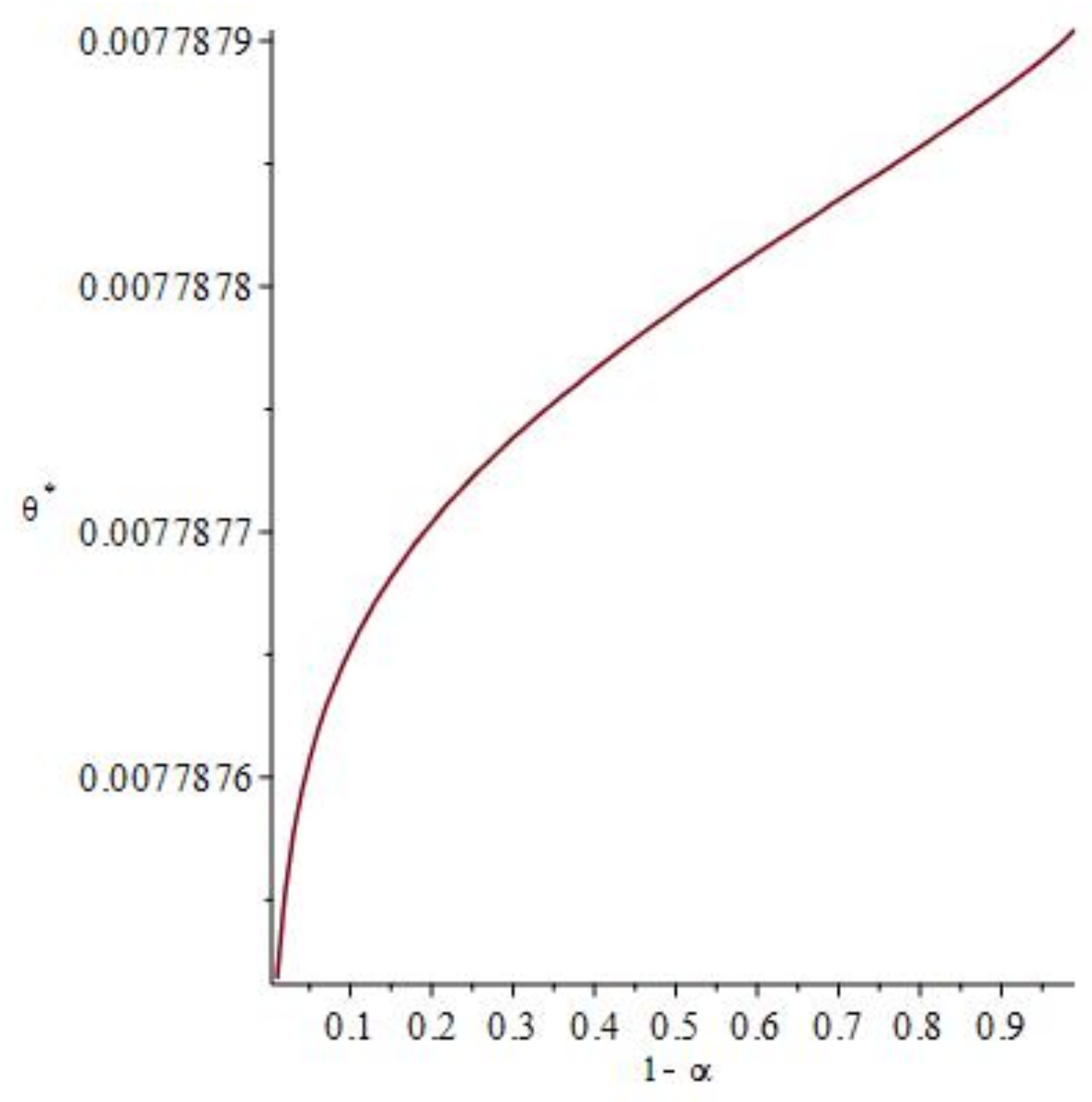
At this point, it is worth investigating the sensitivity of the solution with respect to changes in the confidence level α. This is illustrated in Figure 1 about which we have two observations: First, as the confidence level decreases (i.e. the tolerance level $1-\alpha$ increases), the degree of risk-aversion also decreases and the investor will be willing to take more risk. In this case, the optimal value or income ${\theta }^{*}$ increases to reward the extra risk taken. Second, despite the increase in tolerance level $1-\alpha$, the model is actually robust, this means that, although the values of α vary between 0 and 1, the values of ${\theta }^{*}$ only change marginally. In other words, the variation in the optimal desirable portfolio value is robust with respect to changes in α.

5. Application to Market Integration

Integrated markets should not provide agents with opportunities to make risk-free profits at no cost. The existence of classical arbitrage opportunities is one of the signs that indicate inefficiency in markets. This problem has been investigated in Chen and Knez (1995), and also in Kempf and Korn (1998).

As an alternative to the classical methods, we introduce the indicator ${\theta }^{*}$, i.e., the optimal value of the dual problem, to measure a more general type of inefficiency in markets. From the primal problem, it is clear that $0\le {\theta }^{*}$, a higher value of this quantity indicates a less integrated market in the sense that it leads to opportunities with larger income. By Lemma 1, in an ideal market, the indicator ${\theta }^{*}$ takes a lower value, otherwise, the potential positive income of the portfolio would indicate an inefficiency of the market. To further motivate this indicator, we investigate its relation with the classical arbitrage opportunities.

By Corollary 2, the existence of a desirable portfolio is linked to solving the following system of equations for $(z_v,k_v,\alpha ,\beta )\in {\Delta }_{(\rho ,r)}\times {\mathbb{R}}^{+}\times {\mathbb{R}}^{+}$,

$$k_v=0,p_j=\alpha \beta \mathbb{E}[{\pi }_T^j{z}_v],j=1,2,\dots ,n,$$

where ${\pi }_T^j={\overline{a}}_{.j}·({\mathsf{\Pi }}_T(e_1),\dots ,{\mathsf{\Pi }}_T(e_m))$ and ${\overline{a}}_{.j}=(a_{1j},a_{2j},\dots ,a_{mj})$ is the j-th column of matrix A. If the optimal values satisfy this system of equations then the existence of a desirable opportunity (for a specific risk measure $\rho$) is guaranteed.

Now suppose that the solution set is empty, then by Corollary 2, this means that for any risk measure $\rho$, there is a desirable portfolio. In other words, for such risk measures $\rho$, the existence of desirable portfolios is guaranteed. In this case, it is not difficult to prove that classical arbitrage also exists; see the following corollary.

Corollary 4.

Suppose that the solution set of the following system of equations is empty for $(k_v,z_v,\alpha ,\beta )\in {\Delta }_{(\rho ,r)}\times {\mathbb{R}}^{+}\times {\mathbb{R}}^{+}$,

$$k_v=0,p_j=\alpha \beta \mathbb{E}[{\pi }_T^j{z}_v],j=1,2,\dots ,n,$$

where ${\pi }_T^j={\overline{a}}_{.j}·({\mathsf{\Pi }}_T(e_1),\dots ,{\mathsf{\Pi }}_T(e_m))$ and ${\overline{a}}_{.j}=(a_{1j},a_{2j},\dots ,a_{mj})$ is the j-th column of matrix A. Then, the existence of classical arbitrage in the market is guaranteed.

Example 2.

From Example 1 and based on the available data, one can conclude that Bonds 1 to 4 are consistent in pricing and no desirable portfolio can be built by these bonds. The non-zero ${\theta }^{*}$ for Bonds 1 to 5, indicates inconsistency in pricing, an embedded option, or other hidden risks. Referring to the profile of the bonds in Table 1, one observes that the fifth bond is an inflation indexed note, and the non-zero value of the previous example is indeed indicating the embedded option within this bond. In the next section, specifically Remark 5, we learn how to price this embedded option.

6. Application to Credit Premium Measurement

In this section, we discuss the second application of the theory by measuring the credit risk premium of corporate bonds. As there is an extensive credit risk literature, we only mention the following popular books with many useful references within for interested reader: Bluhm et al. (2010) and Duffie and Singleton (2012). Nevertheless, to the best of our knowledge, the following methodology in measuring credit risk premium, using risk measures, is new.

Suppose that $\{p_1,p_2,\dots ,p_{n-1}\}$ are the current prices of $n-1$ default free bonds (with no embedded option or risk premium) for which we want to use as a base to calculate the credit premium of the defaultable bond $B_n$ (with no embedded options) with the current price $p_n$. Since $B_n$ is defaultable, we have $p_n=q_n-c_p$, where $q_n$ is the price of the bond in the absence of the risk of default, and $c_p$ is the credit premium of the bond that we are interested in estimating. Suppose that our subjective measure of risk is fixed and according to $\rho$, then the following proposition can provide an approximation (a lower bound) to the credit premium. Recall that we have taken the first approach of Section 3.1.

Proposition 1.

If the set of the prices $\{p_1,p_2,\dots ,p_{n-1},q_n\}$ does not provide any desirable portfolio, then $c_p\ge {\theta }^{*}{p}_n$, where ${\theta }^{*}$ is the optimal value of the dual problem in Equation (6) for this set of bonds.

The proof of this proposition is omitted as it follows from the same methodology as in Balbás and López (2008), in particular Propositions 3.1 and 4.1 of their paper. However, their work is not based on a probability model, but the proofs can be adapted to the set up of this proposition.

As it was mentioned earlier, any non-zero optimal value ${\theta }^{*}$ could be due to the existence of a desirable portfolio or other embedded risk premiums such as default risk. However, if we assume that the market is free from any desirable opportunity, then the above proposition can provide an estimation for the credit premiums. Note that the procedure is based on Corollary 2 to estimate these credit premiums. The same procedure can be carried out by Corollary 3. Indeed, applying the latter should provide more accurate credit premiums than with Corollary 2, because it also counts the inconsistencies arising from the existence of strong sequential arbitrage opportunities in the market.

To implement the numerical procedure, we use the risk measure $\rho ={\mathrm{CVaR}}_{\alpha }$ with a confidence level of $\alpha =0.99$, the estimated parameters of Section 4, and the risk statistic DF explained in the last section. We choose a small portfolio as our market.

Remark 5.

The above methodology can be also used to analyze the price of bonds with embedded options. Suppose that $p_n$ is the price of a default-free bond with an embedded option that has a price of $c_p$. Hence, $p_n=q_n+c_p$, where $q_n$ is the price of an equivalent bond without any embedded option. Then, similar to Proposition 1, one can obtain lower bounds for $c_p$.

Example 3.

Suppose that we want to estimate the credit worthiness of Bond 6 in Table 1 with the available data. We already observed in Examples 1 and 2 that Bonds 1 to 4 do not create a desirable portfolio. Therefore, this shows that these bonds are consistently priced with respect to the interest rate model and based on the assumption that there is no desirable opportunity in market; hence they can be used as a benchmark according to Proposition 1 to measure the credit quality of Bond 6 within the available data. For Bonds 1, 2, 3, 4, and 6, the optimization problem in Equation (8) in this case produces an optimal solution of ${\theta }^{*}\approx 0.0044$. Therefore, by Proposition 1, a lower bound for the credit premium of Bond 6 is approximately equal to 0.44.

7. Conclusions

A more general type of opportunity than the classical arbitrage is introduced to build optimal desirable portfolios. Optimization methods and duality theory together with the properties of risk measures are used to create an indicator which can measure this inefficiency in markets. A type of risk statistics is created in order to numerically implement the model in bond markets. The randomness in the bond market is described by an interest rate model. After calibration of the interest rate model, using the US daily treasury yield rates, simulations are used to estimate the sub-gradient set of the risk statistics. Finally, we provide some numerical examples based on real data where both market inefficiencies and the credit quality of a defaultable bond are measured.

References

- Acerbi, Carlo, and Dirk Tasche. 2002. On the coherence of expected shortfall. Journal of Banking & Finance 26: 1487–503. [Google Scholar]
- Ahmed, Shabbir, Damir Filipović, and Gregor Svindland. 2008. A note on natural risk statistics. Operations Research Letters 36: 662–64. [Google Scholar] [CrossRef]
- Artzner, Philippe, Freddy Delbaen, Jean-Marc Eber, and David Heath. 1999. Coherent measures of risk. Mathematical Finance 9: 203–28. [Google Scholar] [CrossRef]
- Assa, Hirbod, and Manuel Morales. 2010. Risk measures on the space of infinite sequences. Mathematics and Financial Economics 2: 253–75. [Google Scholar] [CrossRef]
- Balbás, Alejandro, Beatriz Balbás, and Raquel Balbás. 2010a. Minimizing measures of risk by saddle point conditions. Journal of Computational and Applied Mathematics 234: 2924–31. [Google Scholar] [CrossRef] [Green Version]
- Balbás, Alejandro, Raquel Balbás, and José Garrido. 2010b. Extending pricing rules with general risk functions. European Journal of Operational Research 201: 23–33. [Google Scholar] [CrossRef] [Green Version]
- Balbás, Alejandro, José Garrido, and Silvia Mayoral. 2009. Properties of distortion risk measures. Methodology and Computing in Applied Probability 11: 385–99. [Google Scholar] [CrossRef] [Green Version]
- Balbás, Alejandro, and Susana López. 2008. Sequential arbitrage measurements and interest rate envelopes. Journal of Optimization Theory and Applications 138: 361–74. [Google Scholar] [CrossRef] [Green Version]
- Ben-Tal, Aharon, and Marc Teboulle. 2007. An old-new concept of convex risk measures: The optimized certainty equivalent. Mathematical Finance 17: 449–76. [Google Scholar] [CrossRef]
- Björk, Tomas. 2009. Arbitrage Theory in Continuous Time. New York: Oxford University Press Inc. [Google Scholar]
- Bluhm, Christian, Ludger Overbeck, and Christoph Wagner. 2010. Introduction to Credit Risk Modeling. Boca Raton: CRC Press. [Google Scholar]
- Boero, Gianna, and Costanza Torricelli. 1996. A comparative evaluation of alternative models of the term structure of interest rates. European Journal of Operational Research 93: 205–23. [Google Scholar] [CrossRef]
- Černý, Aleš, and Stewart D. Hodges. 2002. The theory of good-deal pricing in incomplete markets. In Mathematical Finance, Bachelier Congress 2000. Berlin: Springer, pp. 175–202. [Google Scholar]
- Chen, Zhiwu, and Peter J. Knez. 1995. Measurement of market integration and arbitrage. The Review of Financial Studies 8: 287–325. [Google Scholar] [CrossRef]
- Daníelsson, Jón, Bjørn N. Jorgensen, Gennady Samorodnitsky, Mandira Sarma, and Casper G. de Vries. 2013. Fat tails, VaR and subadditivity. Journal of Econometrics 172: 283–91. [Google Scholar] [CrossRef]
- Dhaene, Jan, Roger J. A. Laeven, Steven Vanduffel, Gregory Darkiewicz, and Marc J. Goovaerts. 2008. Can a coherent risk measure be too subadditive? Journal of Risk and Insurance 75: 365–86. [Google Scholar] [CrossRef]
- Duffie, Darrell, and Kenneth J. Singleton. 2012. Credit Risk: Pricing, Measurement, and Management. Princeton: Princeton University Press. [Google Scholar]
- Föllmer, Hans, and Alexander Schi. 2011. Stochastic Finance: An Introduction in Discrete Time. Berlin: Walter de Gruyter GmbH & Co. KG. [Google Scholar]
- Föllmer, Hans, and Stefan Weber. 2015. The Axiomatic approach to risk Measures for capital determination. Annual Review of Financial Economics 7: 301–37. [Google Scholar] [CrossRef]
- Hansen, Lars Peter. 1982. Large sample properties of generalized method of moments estimators. Econometrica 50: 1029–54. [Google Scholar] [CrossRef]
- Kempf, Alexander, and Olaf Korn. 1998. Trading system and market integration. Journal of Financial Intermediation 7: 220–39. [Google Scholar] [CrossRef]
- Kou, Steven, Xianhua Peng, and Chris C. Heyde. 2013. External risk measures and Basel accords. Mathematics of Operations Research 38: 393–417. [Google Scholar] [CrossRef]
- Krätschmer, Volker, Alexander Schied, and Henryk Zähle. 2014. Comparative and qualitative robustness for law-invariant risk measures. Finance and Stochastics 18: 271–95. [Google Scholar] [CrossRef]
- Krokhmal, Pavlo, Jonas Palmquist, and Stanislav Uryasev. 2002. Portfolio optimization with conditional value-at- risk objective and constraints. Journal of Risk 4: 43–68. [Google Scholar] [CrossRef]
- Luenberger, David G. 1969. Optimization by Vector Spaces Methods. New York: John Wiley & Sons. [Google Scholar]
- Markowitz, Harry. 1952. Portfolio selection. Journal of Finance 7: 77–91. [Google Scholar]
- Okhrati, Ramin, and Hirbod Assa. 2017. Representation and approximation of convex dynamic risk measures with respect to strong-weak topologies. Stochastic Analysis and Applications 35: 604–14. [Google Scholar] [CrossRef]
- Protter, Philip E. 2004. Stochastic Integration and Differential Equations. Berlin: Springer-Verlag. [Google Scholar]
- Rockafellar, R. Tyrrell, and Stanislav Uryasev. 2000. Optimization of conditional value-at-risk. Journal of Risk 2: 21–42. [Google Scholar] [CrossRef]
- Rockafellar, R. Tyrrell, and Stanislav Uryasev. 2002. Conditional value-at-risk for general loss distributions. Journal of Banking & Finance 26: 1443–71. [Google Scholar]
- Rockafellar, R. Tyrrell, Stan Uryasev, and Michael Zabarankin. 2006. Generalized deviations in risk analysis. Finance and Stochastics 10: 51–74. [Google Scholar] [CrossRef]
- Sawaragi, Yoshikazu, Hirotaka Nakayama, and Tetsuzo Tanino. 1985. Theory of Multiobjective Optimization (Mathematics in Science and Engineering). Orlando: Academic Press. [Google Scholar]
- Wang, Shaun S. 2000. A class of distortion operators for financial and insurance risks. Journal of Risk and Insurance 67: 15–36. [Google Scholar] [CrossRef]
- Weber, Stefan, William Anderson, A.-M. Hamm, Thomas Knispel, Maren Liese, and Thomas Salfeld. 2013. Liquidity-adjusted risk measures. Mathematics and Financial Economics 7: 69–91. [Google Scholar] [CrossRef]