The Role of Inflation-Indexed Bond in Optimal Management of Defined Contribution Pension Plan During the Decumulation Phase

Abstract

This paper investigates the optimal investment strategy for a defined contribution (DC) pension plan during the decumulation phase which is risk-averse and pays close attention to inflation risk. The plan aims to maximize the expected constant relative risk aversion (CRRA) utility from the terminal real wealth by investing the fund in a financial market consisting of an inflation-indexed bond, an ordinary zero coupon bond and a risk-free asset. We derive the optimal investment strategy in closed-form using the dynamic programming approach by solving the related Hamilton-Jacobi-Bellman (HJB) equation. The results reveal that, with any level of the parameters, an inflation-indexed bond has significant advantage to hedge inflation risk.

1. Introduction and Motivation

An asset allocation problem incorporating inflation risk for individual investors has been studied by many researchers. A closed form of optimal investment strategy is given by Brennan and Xia (2002), then Munk et al. (2004) obtain the optimal strategy in a model with inflation uncertainty by the dynamic programming method. Since differences in spending patterns and in price increases lead to unequal inflation experiences, the work of Li et al. (2017) considers an optimal investment and consumption problem of households under inflation inequality.

Inflation-indexed bond is defined as an financial instrument that delivers a defined payoff indexed by inflation at maturity time, which can be utilized to hedge against inflation risk. For an investment company, Nkeki and Nwozo (2013) find that inflation risk associated with investment could be hedged by investing in inflation-linked bond, with some assumptions of stochastic cash inflows and outflows of the company. Liang and Zhao (2016) investigate the efficient frontier and optimal strategies of a family under mean-variance efficiency, and the work of Pan and Xiao (2017) deals with an optimal asset-liability management problem. Both works mentioned above take into account the inflation risk and consider the problem in the real market instead of the nominal price.

Such kind of bonds are applied in life insurance. Kwak and Lim (2014) investigate a continuous time optimal consumption, investment and life insurance decision problem of a family under inflation risk, which explicit solutions are derived by using martingale method. Then Han and Hung (2017) solve a similar investment problem of a wage earner before retirement with the method of dynamic programming approach. In order to hedge against inflation risk, an inflation-indexed bond is introduced in both two problems above.

In order to guarantee consumptions for oneself after retirement, or for his or her beneficiaries (spouse, children or parents), a pension plan is introduced as an organized and systematic financial instrument to provide regular incomes. In the dimension of benefits, there are two principal types of pension plans: defined contribution (DC) and defined benefit (DB). In the DC case, benefits are generated by the accumulation of contributions, and contributions paid by the pension member are defined explicitly. Optimal investment decision problems are studied by many works for DC pension plan. For instance, the work of Sun et al. (2017) deals with the portfolio optimization problem by investing the pension fund in a market consisting of various government and corporate bonds, allowing for the possibility of bond defaults. The work of Guan and Liang (2016) studies the stochastic Nash equilibrium portfolio game between two DC pension schemes under inflation risks.

However, for DB type pension scheme, benefits received after retirement are defined explicitly by the rules of the scheme. There are also lots of works about optimal management on DB pension. For example, in order to minimize deviations of the unfunded actuarial liability, Josa-Fombellida and Rincón-Zapatero (2010) consider optimal portfolio decision problem for an aggregated DB pension plan in the framework of stochastic interest rate.

In the dimension of funding, there are also two types of pension fund: pay as you go (PAYG) and funding. In a PAYG mechanism, contributions paid by the active affiliates are directly used as retired people’s benefits. Optimal management in PAYG mechanism are introduced by many researchers. For instance, by applying optimal control techniques, Haberman and Zimbidis (2002) develop a deterministic-continuous model and a stochastic-discrete model using a contingency fund. To guarantee the required level of liquidity, Godínez-Olivares et al. (2016) design optimal strategies using nonlinear dynamic programming through changes in the key variables of pension system (contribution rate, retirement age and indexation). Other works in PAYG mechanism can be found in the works of Alonso-García and Devolder (2016) and Alonso-García et al. (2017).

However, in a funding mechanism, contributions paid by a group of people are invested in the financial market and will be used as their own benefits. There are also many works in optimal management problems. The work of Li et al. (2016) aims to derive optimal time-consistent investment strategy under the mean-variance criterion, by investing pension wealth in a financial market consisting of a bank account and a risky asset (which price process satisfies the constant elasticity of variance model). Other works in funding mechanism are studied by Sun et al. (2016,2017).

As the investment of a DC pension plan involves quite a long period of time, it seems implausible to ignore inflation risk in the long run. Moreover, in a DC pension plan, benefits depend solely on the returns of the fund’s portfolio, so it is meaningful to protect inflation risk in such kind of pension scheme. Yao et al. (2013) solve a mean-variance problem by considering the real wealth process including the influence of inflation. Okoro and Nkeki (2013) examine the optimal variational Merton portfolios with inflation protection strategy. Both expected values of pension plan member’s terminal wealth and efficient frontier are obtained in their work.

Generally, a pension scheme contains an accumulation (contribution) phase, which is the period before retirement, and a decumulation (distribution) phase, which is the period after retirement. There are some applications of inflation bond in pension plans which concentrate on the optimal management during the accumulation phase. Zhang et al. (2007) and Zhang and Ewald (2010) investigate an optimal investment problem by investing an indexed bond, and present a way to deal with the optimization problem using the martingale method. In the work of Han and Hung (2012), stochastic dynamic programming approach is used to investigate the optimal asset allocation for a DC pension plan with downside protection under stochastic inflation, and the inflation-indexed bond is again included in the asset menu to cope with the inflation risk. According to Chen et al. (2017), an optimal investment strategy for a DC plan member who pays close attention to inflation risks and requires a minimum performance at retirement is solved by martingale approach. Another applications of inflation-indexed bond can be found in Nkeki (2018) and Tang (2018).

As the decumulation phase of a DC pension scheme is also confronted with inflation risk, this paper applies the inflation bond in this period and considers an optimal control problem, which continuously decides weights of investment in different assets, including a zero coupon bond, an inflation-indexed bond and a riskless asset, in order to maximize the terminal wealth with the consideration of the influence of inflation.

Another motivation of our work is to investigate whether the investment efficiency is improved by the inflation-index bond. The question is whether the optimal utility function is increased with the investment of the index bond. In order to do the comparative study, we follow the definition of the indexed bond price, see, for instance, Nkeki and Nwozo (2013) or Han and Hung (2017), but find another SDE to describe its price. In our work, the price of an ordinary bond is just a special case of the price of the indexed bond.

The rest of the paper is structured as follows. Section 2 describes the financial market with stochastic interest rate, stochastic price level and three tradable assets which are of interest for our problem. The demographic pattern is given by a drifted Brownian motion. Section 3 solves an optimal investment problem with investment in a complete market including an inflation-indexed bond, an ordinary zero coupon bond and a bank account. The closed form solutions of this stochastic control problem are given by solving the related HJB equation. The counterpart, Section 4 solves a similar problem with the indexed bond excluded. Section 5 gives the sensitivity analysis. At last, Section 6 compares the results given by Section 3 and Section 4 and gives the conclusion. The comparative study shows that investment in the indexed bond has significant advantage to hedge inflation risk.

2. Model Assumptions and Notations

2.1. The Financial Market

The instantaneously nominal interest rate $R(t)$ is assumed to be stochastic. Here we use the Ornstein-Uhlenbeck process introduced by Vasicek (1997), i.e., $R(t)$ satisfies the following differential equation:

$$\begin{array}{c}\hfill \begin{array}{c}\hfill dR(t)=b\left(a-R(t)\right)dt+{\sigma }_{R}d{Z}_1(t)\end{array}\end{array}$$

(1)

where $Z_1(t)$ is a standard Brownian motion under probability measure P, $R(0)=R_0$ and all parameters are assumed to be positive constants.

Assume there is a financial market consisting of three tradable underlying instruments which are traded continuously over time and are perfectly divisible. In addition, we assume that there are no transaction costs or taxes in the context. Borrowing and short-selling are permitted.

a. A money market account $M(t)$ satisfies the following equation:

$$\begin{array}{c}\hfill \begin{array}{c}\hfill {\displaystyle \frac{dM(t)}{M(t)}}=R(t)dt\end{array}\end{array}$$

(2)

with initial value $M(0)=M_0$.

b. A zero coupon nominal bond which pays one monetary unit at expiration time $T_0$, and its value $B(t,T_0)$ at time t can be written as the conditional expectation under the so-called equivalent martingale measure corresponding to the arbitrage free market, under which $e^{-{\int }_0^{t}R(u)du}B(t,T_0)$ is a local martingale:

$$\begin{array}{c}\hfill \begin{array}{c}\hfill B(t,T_0)={\mathbb{E}}_Q\left\{e^{-{\int }_t^{T_0}R(u)du}|{\mathcal{F}}_t\right\}\end{array}\end{array}$$

(3)

Considering the martingale property of the discounting process of $B(t,T_0)$ and following the work of Menoncin (2008), we get the dynamics of the bond price:

$$\begin{array}{c}\hfill \begin{array}{ccc}\hfill dB(t,T_0)& =& B(t,T_0)R(t)dt+{\displaystyle \frac{\partial B(t,T_0)}{\partial R(t)}}{\sigma }_{R}d{Z}_1^Q(t)\hfill \\ \hfill B(T_0,T_0)& =& 1\hfill \end{array}\end{array}$$

(4)

where $Z_1^Q(t)$ is a standard Brownian motion under measure Q. Let ${\lambda }_R$ be the market price for the interest rate risk, then by Girsanov’s theorem, $d{Z}_1^Q(t)={\lambda }_{R}dt+d{Z}_1(t)$ is a Wiener process. The Radon-Nikodym derivative is defined by $\Lambda (T_0)=\frac{dQ}{dP}(Z_1[0,T_0])=exp\left\{-{\lambda }_R{Z}_1(T_0)-\frac{1}{2}{\lambda }_R^2{T}_0\right\}$. Consequently, one can get the stochastic differential equation of $B(t,T_0)$ under the original measure P:

$$\begin{array}{c}\hfill \begin{array}{ccc}\hfill {\displaystyle \frac{dB(t,T_0)}{B(t,T_0)}}& =& \left(R(t)+{\nabla }_R^B(t){\sigma }_R{\lambda }_R\right)dt+{\nabla }_R^B(t){\sigma }_{R}d{Z}_1(t)\hfill \\ \hfill B(T_0,T_0)& =& 1\hfill \end{array}\end{array}$$

(5)

where ${\nabla }_R^B(t)=\frac{\partial B(t,T_0)}{\partial R(t)}\frac{1}{B(t,T_0)}$ is the semi-elasticity of the bond price with respect to the interest rate, which is a negative function of time t, because the bond negatively reacts to the shocks on interest rate.

Remark 1.

Since the bond has a positive premium compared with the riskless asset, ${\lambda }_R$ is assumed to be negative.

c. With regards to the stochastic price level, we define the inflation index (or the level of consumer price) process as:

$$\begin{array}{c}\hfill \begin{array}{c}\hfill {\displaystyle \frac{dP(t)}{P(t)}}=i(t)dt+{\sigma }_{P}d{Z}_2(t)\end{array}\end{array}$$

(6)

with $P(0)=P_0>0$. $i(t)$ is a deterministic function of time t representing the expected rate of inflation and ${\sigma }_P$ is the constant volatility. $Z_2(t)$ is another Brownian motion under the physical measure P, which generates uncertainty in the price level and is independent of $Z_1(t)$. If we set ${\lambda }_p$ as the market price of risk with respect to $d{Z}_2(t)$, then $d{Z}_2^Q(t)={\lambda }_{P}dt+d{Z}_2(t)$ is a Wiener process, where $Z_2^Q(t)$ is a Brownian motion under the risk neutral measure Q. $P(t)$ has the explicit form as the following:

$$\begin{array}{c}\hfill \begin{array}{c}\hfill P(t)=P_{0}exp\left\{{\displaystyle {\int }_0^{t}i(s)ds-({\sigma }_P{\lambda }_p+{\displaystyle \frac{{{\sigma }_P}^2}{2}})t+{\sigma }_P{Z}_2^Q(t)}\right\}\end{array}\end{array}$$

(7)

As in the work of Han and Hung (2012), we define an inflation-indexed zero coupon bond, whose price at time t is denoted by $I(t,T_0)$, from which the investor can get $P_{T_0}$ units of money at the maturity time $T_0$. By the fundamental theorem of asset pricing, it is well known that in an arbitrage free market the price of any asset coincides with the expected present value of its future cash flows under the equivalent martingale measure Q. Thus, we have

$$\begin{array}{c}\hfill \begin{array}{ccc}\hfill I(t,T_0)& =& {\mathbb{E}}_Q\left\{P_{T_0}{e}^{-{\int }_t^{T_0}R(u)du}|{\mathcal{F}}_t\right\}\hfill \\ \hfill & =& P_0{e}^{{\int }_0^{T_0}i(s)ds-({\sigma }_P{\lambda }_P+{{\sigma }_P}^2/2)T_0}{e}^{{\sigma }_P{Z}_2^Q(t)}{\mathbb{E}}_Q\left\{e^{{\sigma }_P\left(Z_2^Q(T_0)-Z_2^Q(t)\right)}{e}^{-{\int }_t^{T_0}R(u)du}|{\mathcal{F}}_t\right\}\hfill \end{array}\end{array}$$

(8)

Lemma 1.

In Equation (8),

$$\begin{array}{c}\begin{array}{cc}& {\mathbb{E}}_Q\left\{e^{{\sigma }_P\left(Z_2^Q(T_0)-Z_2^Q(t)\right)}{e}^{-{\int }_t^{T_0}R(u)du}|{\mathcal{F}}_t\right\}\hfill \\ \hfill =& {\mathbb{E}}_Q\left\{e^{{\sigma }_P\left(Z_2^Q(T_0)-Z_2^Q(t)\right)}\right\}{\mathbb{E}}_Q\left\{e^{-{\int }_t^{T_0}R(u)du}|{\mathcal{F}}_t\right\}\hfill \\ \hfill =& e^{{\sigma }_P^2(T_0-t)/2}B(t,T_0)\hfill \end{array}\end{array}$$

(9)

Proof. 

Denote ${\mathcal{F}}_t^1=\sigma \left\{Z_1^Q(s),s\le t\right\}$, ${\mathcal{F}}_t^2=\sigma \left\{Z_2^Q(s),s\le t\right\}$, and set ${\mathcal{F}}_t={\mathcal{F}}_t^1\vee {\mathcal{F}}_t^2$. Since $e^{-{\int }_t^{T_0}R(u)du}$ is independent of $e^{{\sigma }_P\left(Z_2^Q(T_0)-Z_2^Q(t)\right)}$ and ${\mathcal{F}}_t^2$, and ${\mathcal{F}}_t^1$ is independent of ${\mathcal{F}}_t^2$, we have:

$$\begin{array}{ll}& {\mathbb{E}}_Q\left\{e^{{\sigma }_P\left(Z_2^Q(T_0)-Z_2^Q(t)\right)}{e}^{-{\int }_t^{T_0}R(u)du}|{\mathcal{F}}_t\right\}\\ =& {\mathbb{E}}_Q\left\{e^{-{\int }_t^{T_0}R(u)du}|{\mathcal{F}}_t^1\right\}{\mathbb{E}}_Q\left\{e^{{\sigma }_P\left(Z_2^Q(T_0)-Z_2^Q(t)\right)}|{\mathcal{F}}_t^2\right\}.\end{array}$$

(10)

Since $R(t)$ is independent of ${\mathcal{F}}_t^2$, we have ${\mathbb{E}}_Q\left\{e^{-{\int }_t^{T_0}R(u)du}|{\mathcal{F}}_t^1\right\}={\mathbb{E}}_Q\left\{e^{-{\int }_t^{T_0}R(u)du}|{\mathcal{F}}_t\right\}$. ${\mathcal{F}}_t^2$ disappears in the second part because of the property of independent increment of a Brownian motion, and the last equality of (9) holds by the property of exponential martingale. ☐

At last, we get a formulation of $I(t,T_0)$ related with $B(t,T_0)$:

$$\begin{array}{c}\hfill I(t,T_0)=P_0{e}^{{\int }_0^{T_0}i(s)ds-{\sigma }_P{\lambda }_P{T}_0}{e}^{-{{\sigma }_P}^{2}t/2}{e}^{{\sigma }_P{Z}_2^Q(t)}B(t,T_0)\end{array}$$

(11)

By the chain rule of Itô’s formula, the evolution of $I(t,T_0)$ is described by the following stochastic differential equation:

$$\begin{array}{c}\hfill dI(t,T_0)=P_0{e}^{{\int }_0^{T_0}i(s)ds-{\sigma }_P{\lambda }_P{T}_0}\left[e^{-{{\sigma }_P}^{2}t/2}{e}^{{\sigma }_P{Z}_2^Q(t)}dB(t,T_0)+e^{-{{\sigma }_P}^{2}t/2}B(t,T_0){\sigma }_P{e}^{{\sigma }_P{Z}_2^Q(t)}d{Z}_2^Q(t)\right]\end{array}$$

(12)

Finally, we have:

$$\begin{array}{cc}\hfill {\displaystyle \frac{dI(t,T_0)}{I(t,T_0)}}& ={\displaystyle \frac{dB(t,T_0)}{B(t,T_0)}}+{\sigma }_{P}d{Z}_2^Q(t)\hfill \\ & =\left(R(t)+{\nabla }_R^B{\sigma }_R{\lambda }_R+{\sigma }_P{\lambda }_P\right)dt+{\nabla }_R^B{\sigma }_{R}d{Z}_1(t)+{\sigma }_{P}d{Z}_2(t)\hfill \end{array}$$

(13)

Thus, we get a correlation between the price of the inflation-indexed bond and that of an ordinary zero coupon bond.

2.2. The Demographic Pattern

As to the demographic pattern, a meaningful and concise structure is presented in the work of Zimbidis and Pantelous (2008). It is assumed that the dynamic of number of death follows a stochastic differential equation:

$$\begin{array}{c}\hfill -dl(t)=\theta (t)dt+\nu (t)d{Z}_3(t)\end{array}$$

(14)

where $\theta (t)$ and $\nu (t)$ describe the instantaneous drift and volatility, respectively. $Z_3(t)$ is another standard Brownian motion under measure P, which is independent of $Z_1(t)$ and $Z_2(t)$.

Remark 2.

As for the demographic pattern, more advanced structure is considered in the work of Pantelous and Zimbidis (2009). The dynamic of the number of death follows $-dl(t)=\theta (t)dt+\nu (t)d{B}^{\mathcal{H}}(t)$, with $B^{\mathcal{H}}(t)$ a fractional Brownian motion, which is more significant since it can model observed long-range dependence of large family of stochastic processes in a simple way by the property of long memory.

Now set ${\mathcal{F}}_t={\mathcal{F}}_t^1\vee {\mathcal{F}}_t^2\vee {\mathcal{F}}_t^3$, where ${\mathcal{F}}_t^3=\sigma \left\{Z_3^Q(s),s\le t\right\}$. It is not hard to show that the result in Lemma 1 still holds.

3. DC Pension Fund Management with Investment of Inflation-Indexed Bond

In a DC pension scheme, see, for example, Zimbidis and Pantelous (2008), a plan member pays contributions during his or her employment period and beneficiaries of each pensioner (who dies at time t) receive an accumulated amount, as a whole life assurance with a death benefit.

Here we consider a stochastic control problem with finite time horizon, in order to maximize the terminal expected utility wealth and find optimal investment policies for assets in the decumulation phase of the pension plan, from modeling time $t=0$ to a suitable terminal time $t=T(T\le T_0)$. With the investment of the ordinary bond and the inflation-indexed bond, the financial market is complete. The market can be represented as the following matrix form:

$$\left[\begin{array}{c}{\displaystyle \frac{dB}{B}}\\ {\displaystyle \frac{dI}{I}}\end{array}\right]=\left[\begin{array}{c}R+{\nabla }_R^B{\sigma }_R{\lambda }_R\\ R+{\nabla }_R^B{\sigma }_R{\lambda }_R+{\sigma }_P{\lambda }_P\end{array}\right]dt+\underset{\Sigma }{\underbrace{\left[\begin{array}{cc}{\nabla }_R^B{\sigma }_R& 0\\ {\nabla }_R^B{\sigma }_R& {\sigma }_P\end{array}\right]}}\left[\begin{array}{c}d{Z}_1\\ d{Z}_2\end{array}\right]$$

(15)

where the matrix $\Sigma$ is invertible.

It is easily to get the following equation which describes the evolution of the fund:

$$\begin{array}{ccc}dX(t)\hfill & =\hfill & \left(1-u_1^{BI}(t)-u_2^{BI}(t)\right)X(t){\displaystyle \frac{dM(t)}{M(t)}}+u_1^{BI}(t)X(t){\displaystyle \frac{dB(t,T_0)}{B(t,T_0)}}\hfill \\ \hfill & & +u_2^{BI}(t)X(t){\displaystyle \frac{dI(t,T_0)}{I(t,T_0)}}-X(t)c(t)\left(-dl(t)\right)\hfill \\ \hfill & =\hfill & X(t)\left[R(t)+u_1^{BI}(t){\nabla }_R^B(t){\sigma }_R{\lambda }_R+u_2^{BI}(t)({\nabla }_R^B(t){\sigma }_R{\lambda }_R+{\sigma }_P{\lambda }_P)-c(t)\theta (t)\right]dt\hfill \\ \hfill & & +X(t)\left(u_1^{BI}(t)+u_2^{BI}(t)\right){\nabla }_R^B(t){\sigma }_{R}d{Z}_1(t)+X(t)u_2^{BI}(t){\sigma }_{P}d{Z}_2(t)-X(t)c(t)\nu (t)d{Z}_3(t)\hfill \\ X(0)\hfill & =\hfill & X_0\hfill \end{array}$$

(16)

where $c(t)$ is the weight of benefit received immediately by the beneficiaries, i.e., the benefit associated with the pension fund is assumed to be a deterministic proportion $c(t)$ of the pension wealth. With this assumption, the pension sponsor pays more benefits with a higher investment income, and pays less benefits with a lower investment income, which makes the pension plan realistic and attractive to the individual.

$u_1^{BI}(t)$ and $u_2^{BI}(t)$ are weights invested into the ordinary zero coupon bond and the inflation-index bond at time t, respectively. A negative value of $u_1^{BI}$ or $u_2^{BI}$ means that the sponsor takes a short position in the ordinary bond or the indexed bond, respectively, while a negative value of $1-u_1^{BI}-u_2^{BI}$ means that in order to buy ordinary bond or indexed bond, the sponsor borrows from the bank at the rate R. Denote $u^{BI}(t)=\left(u_1^{BI}(t),u_2^{BI}(t)\right)$. It is called admissible if it satisfies the following conditions, and we denote the set of all admissible controls by $\Pi$.

• $u^{BI}(t)$ is progressively measurable with respect to ${\left\{{\mathcal{F}}_t\right\}}_{t\ge 0}$;
• $\mathbb{E}\left\{{\displaystyle {\int }_0^T\left[{\left(X(t)\left(u_1^{BI}(t)+u_2^{BI}(t)\right){\nabla }_R^B{\sigma }_R\right)}^2+{\left(X(t)u_2^{BI}(t){\sigma }_P\right)}^2+{\left(X(t)c(t)\nu (t)\right)}^2\right]dt}\right\}<\infty ;$
• Equation (16) has a unique strong solution for the initial value $(t_0,R_0,X_0)\in [0,T]\times {(0,\infty )}^2$.

As mentioned in Section 1, the control period for the pension fund is very long, hence the effect of inflation becomes noticeable for the pension manager. Denote the real wealth process including the impact of inflation by $\overline{X}(t)$, i.e., $\overline{X}(t)=X(t)/P(t)$. By the chain rule, we have that $\overline{X}(t)$ follows:

$$\begin{array}{ccc}\hfill {\displaystyle \frac{d\overline{X}(t)}{\overline{X}(t)}}& =& \left[R(t)+u_1^{BI}(t){\nabla }_R^B(t){\sigma }_R{\lambda }_R+u_2^{BI}(t)({\nabla }_R^B(t){\sigma }_R{\lambda }_R+{\sigma }_P{\lambda }_P-{\sigma }_P^2)-c(t)\theta (t)+{\sigma }_P^2-i(t)\right]dt\hfill \\ & & +\left(u_1^{BI}(t)+u_2^{BI}(t)\right){\nabla }_R^B(t){\sigma }_{R}d{Z}_1(t)+\left(u_2^{BI}(t){\sigma }_P-{\sigma }_P\right)d{Z}_2(t)-c(t)\nu (t)d{Z}_3(t)\hfill \\ \hfill \overline{X}(0)& =& X_0/P_0\hfill \end{array}$$

(17)

The pension sponsor would like to maximize the expected utility of terminal real fund $\overline{X}(t)$. Our optimal problem can be written as:

$$\begin{array}{c}\hfill \underset{\left\{u^{BI}\in \Pi \right\}}{max}\mathbb{E}\left[U(\overline{X}(T))\right]\end{array}$$

(18)

where $U(x)$ is the utility function which describes the preference over wealth. Here we consider the typical CRRA utility function, for which we can derive the explicit form of the solution, as follows:

$$\begin{array}{c}\hfill U(x)={\displaystyle \frac{x^{1-\gamma }}{1-\gamma }},\gamma >0and\gamma \ne 1,\end{array}$$

(19)

where $\gamma$ is the relative risk aversion.

Remark 3.

For simplicity, we do not consider any risk-based regulatory constraints such as those in the Solvency II Directive in this paper, though it is more realistic in financial and insurance market. To consider financial regulation problems, for instance, Duarte et al. (2017) propose an asset and liability management model with a thorough representation of a risk-based regulation by applying the multistage stochastic programming model.

The problem can be solved by the dynamic programming method. Denote $V(t,R,x)=\mathbb{E}\left\{U(\overline{X}(T))|\overline{X}(t)=x,R(t)=R\right\}$ as the value function. In stochastic optimal control theory, the HJB equation accomplishes the connection between the value function and the optimal control, see Fleming and Soner (1993) or Yong and Zhou (1999). Denote $u_1^{BI}(t)=u_1^{BI}$, $u_2^{BI}(t)=u_2^{BI}$, ${\nabla }_R^B(t)={\nabla }_R^B$ and so on, we have the associated HJB equation for the above problem as follows:

$$\begin{array}{c}\hfill \underset{\left\{u^{BI}\in \Pi \right\}}{max}\Psi (u_1^{BI},u_2^{BI})=0\end{array}$$

(20)

where

$$\begin{array}{cc}\hfill \Psi (u_1^{BI},u_2^{BI})=& V_t+V_{x}x\left[R+u_1^{BI}{\nabla }_R^B{\sigma }_R{\lambda }_R+u_2^{BI}({\nabla }_R^B{\sigma }_R{\lambda }_R+{\sigma }_P{\lambda }_P-{\sigma }_P^2)-c\theta +{\sigma }_P^2-i\right]\hfill \\ & +{\displaystyle \frac{1}{2}}{V}_{xx}{x}^2\left[{\left(u_1^{BI}+u_2^{BI}\right)}^2{{\nabla }_R^B}^2{{\sigma }_R}^2+{(u_2^{BI}{\sigma }_P-{\sigma }_P)}^2+c^2{\nu }^2\right]\hfill \\ & +V_{R}b(a-R)+{\displaystyle \frac{1}{2}}{V}_{RR}{{\sigma }_R}^2+V_{Rx}x(u_1^{BI}+u_2^{BI}){\nabla }_R^B{{\sigma }_R}^2=0\hfill \end{array}$$

(21)

with terminal condition $V(T,R,x)=\frac{x^{1-\gamma }}{1-\gamma }$. $V_t$, $V_x$, $V_R$, $V_{xx}$, $V_{RR}$ and $V_{Rx}$ denote the first and second order partial derivatives of V with respect to t, x and R, respectively.

The maximization of $\Psi (u_1^{BI},u_2^{BI})$ can be obtained by the optimal functional ${u_1^{BI}}^{*}$ and ${u_2^{BI}}^{*}$, which satisfy the following necessary conditions:

$$\begin{array}{c}\hfill \Psi ({u_1^{BI}}^{*},{u_2^{BI}}^{*})=0\\ \hfill {\displaystyle \frac{d\Psi }{d{u}_1^{BI}}}({u_1^{BI}}^{*})=0\\ \hfill {\displaystyle \frac{d\Psi }{d{u}_2^{BI}}}({u_2^{BI}}^{*})=0\end{array}$$

(22)

The first order conditions expressed as feedback formulas in term of derivatives of the value function are:

$$\begin{array}{c}{u_1^{BI}}^{*}=-{\displaystyle \frac{V_x}{V_{xx}x}}{\displaystyle \frac{{\lambda }_R}{{\nabla }_R^B{\sigma }_R}}-{\displaystyle \frac{V_{Rx}}{V_{xx}x}}{\displaystyle \frac{1}{{\nabla }_R^B}}-{\displaystyle \frac{V_x}{V_{xx}x}}{\displaystyle \frac{{\sigma }_P-{\lambda }_P}{{\sigma }_P}}-1\hfill \\ {u_2^{BI}}^{*}={\displaystyle \frac{V_x}{V_{xx}x}}{\displaystyle \frac{{\sigma }_P-{\lambda }_P}{{\sigma }_P}}+1\hfill \end{array}$$

(23)

Substituting Equation (23) into the HJB Equation (20), we can finally get the explicit forms of the value function and the optimal investment strategies. They are given in the following theorem.

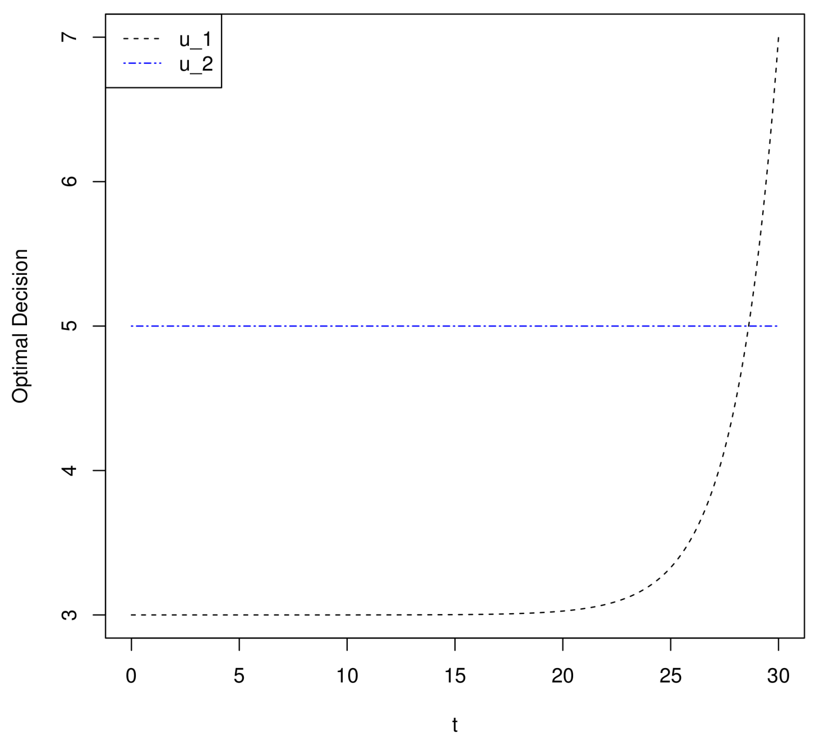
Theorem 1.

The optimal utility and optimal investment strategies are given by

$$\begin{array}{ccc}\hfill V(t,R,x)& =& {\displaystyle \frac{x^{1-\gamma }}{1-\gamma }}{e}^{A_1^{BI}(t)+A_2^{BI}(t)R}\hfill \\ \hfill {u_1^{BI}}^{*}(t)& =& {\displaystyle \frac{1}{\gamma }}{\displaystyle \frac{{\lambda }_R}{{\nabla }_R^B{\sigma }_R}}+{\displaystyle \frac{1}{\gamma }}{\displaystyle \frac{1}{{\nabla }_R^B}}{A}_2^{BI}(t)+{\displaystyle \frac{1}{\gamma }}{\displaystyle \frac{{\sigma }_P-{\lambda }_P}{{\sigma }_P}}-1\hfill \\ \hfill {u_2^{BI}}^{*}(t)& =& {\displaystyle \frac{1}{\gamma }}{\displaystyle \frac{{\sigma }_P-{\lambda }_P}{{\sigma }_P}}+1\hfill \end{array}$$

(24)

where

$$\begin{array}{c}\hfill A_2^{BI}(t)=-{\displaystyle \frac{1-\gamma }{b}}\left[e^{-b(T-t)}-1\right]\end{array}$$

(25)

$$\begin{array}{c}\hfill {\displaystyle A_1^{BI}(t)={\int }_t^T{\alpha }^{BI}(s)ds}\end{array}$$

(26)

$$\begin{array}{cc}\hfill {\alpha }^{BI}(t)=& {\displaystyle \frac{1}{2}}{\displaystyle \frac{1-\gamma }{\gamma }}\left({\lambda }_R^2+{({\sigma }_P-{\lambda }_P)}^2\right)+(1-\gamma )({\sigma }_P{\lambda }_P-c\theta -i)-{\displaystyle \frac{1}{2}}\gamma (1-\gamma )c^2{\nu }^2\hfill \\ & +A_2^{BI}(t)ba+{\displaystyle \frac{1}{2}}{A_2^{BI}(t)}^2{\sigma }_R^2+{\displaystyle \frac{1-\gamma }{\gamma }}{A}_2^{BI}(t){\lambda }_R{\sigma }_R+{\displaystyle \frac{1}{2}}{\displaystyle \frac{1-\gamma }{\gamma }}{A_2^{BI}(t)}^2{\sigma }_R^2\hfill \end{array}$$

(27)

Proof. 

See Appendix A. ☐

Figure 1 shows the time-varying optimal weights of $u_1^{BI}$ and $u_2^{BI}$, from which we can see that ${u_1^{BI}}^{*}$ increases exponentially with time t, while ${u_2^{BI}}^{*}$ is independent of time t (with ${\nabla }_R^B=-0.5$, ${\lambda }_R=-0.5$, ${\lambda }_P=0.5$, $\gamma =0.5$ and $b=0.5$).

In order to do some comparison with Section 4, we denote $V(t,R,x)\triangleq V^{BI}(t,R,x)$.

4. DC Pension Fund Management without the Investment of Inflation-indexed Bond

In order to investigate the role of the inflation-linked bond in pension management, we consider another optimal portfolio selection problem with the indexed bond excluded in this section. Here we abuse the notation and set the wealth process again denoted by $X(t)$, but the portfolio only consists of a bank account and an ordinary T-bond. In this case the financial market is incomplete: there is no enough assets for hedging against the inflation risk, i.e., the stochasticity $Z_2$. The financial assets in the market can be summarized in the following matrix form:

$$\frac{dB}{B}=\left[\begin{array}{c}R(t)+{\nabla }_R^B{\sigma }_R{\lambda }_R\end{array}\right]dt+\underset{\Sigma }{\underbrace{\left[\begin{array}{cc}{\nabla }_R^B{\sigma }_R& 0\end{array}\right]}}\left[\begin{array}{c}d{Z}_1\\ d{Z}_2\end{array}\right]$$

(28)

in which case the matrix $\Sigma$ is not invertible. Actually, there does not exist any linear combination of assets to replicate the inflation risk.

Similarly, the corresponding wealth process can be defined as:

$$\begin{array}{ccc}\hfill dX(t)& =& \left(1-u_1^B(t)\right)X(t){\displaystyle \frac{dM(t)}{M(t)}}+u_1^B(t)X(t){\displaystyle \frac{dB(t,T_0)}{B(t,T_0)}}-X(t)c(t)\left(-dl(t)\right)\hfill \\ \hfill & =& X(t)\left[R(t)+u_1^B(t){\nabla }_R^B(t){\sigma }_R{\lambda }_R-c(t)\theta (t)\right]dt+X(t)u_1^B(t){\nabla }_R^B(t){\sigma }_{R}d{Z}_1(t)\hfill \\ & & -X(t)c(t)\nu (t)d{Z}_3(t)\hfill \\ \hfill X(0)& =& X_0\hfill \end{array}$$

(29)

where $u_1^B(t)$ describes the weight allocated to the zero coupon bond.

Again denote the real wealth process including the impact of inflation by $\overline{X}(t)$, and by the chain rule, its dynamic is

$$\begin{array}{ccc}\hfill {\displaystyle \frac{d\overline{X}(t)}{\overline{X}(t)}}& =& \left[R(t)+u_1^B(t){\nabla }_R^B(t){\sigma }_R{\lambda }_R-c(t)\theta (t)+{\sigma }_P^2-i(t)\right]dt+u_1^B(t){\nabla }_R^B(t){\sigma }_{R}d{Z}_1(t)\hfill \\ \hfill & & -{\sigma }_{P}d{Z}_2(t)-c(t)\nu (t)d{Z}_3(t)\hfill \\ \hfill \overline{X}(0)& =& X_0/P_0\hfill \end{array}$$

(30)

We have exactly the same objective function and the same optimization problem in Section 3 and Section 4, except that the investment of an inflation-indexed bond has been removed. Analogously, denote $u_1^{BI}(t)=u_1^{BI}$, $u_2^{BI}(t)=u_2^{BI}$, ${\nabla }_R^B(t)={\nabla }_R^B$ and so on, the related HJB equation is

$$\begin{array}{cc}\hfill \underset{\left\{u^B\in \Pi \right\}}{max}& V_t+V_{x}x\left(R+u_1^B{\nabla }_R^B{\sigma }_R{\lambda }_R-c\theta +{\sigma }_P^2-i\right)+{\displaystyle \frac{1}{2}}{V}_{xx}{x}^2\left[{u_1^B}^2{{\nabla }_R^B}^2{\sigma }_R^2+{{\sigma }_P}^2+c^2{\nu }^2\right]\hfill \\ & +V_{R}b(a-R)+{\displaystyle \frac{1}{2}}{V}_{RR}{{\sigma }_R}^2+V_{Rx}x{u}_1^B{\nabla }_R^B{{\sigma }_R}^2=0\hfill \end{array}$$

(31)

where $V(t,R,x)$ is again the value function corresponding the optimal problem with terminal condition $V(T,R,x)=\frac{x^{1-\gamma }}{1-\gamma }$.

By differentiating with respect to $u_1^B$, the optimal weight can be expressed in the form of the value function:

$$\begin{array}{c}\hfill {u_1^B}^{*}=-{\displaystyle \frac{V_x}{V_{xx}x}}{\displaystyle \frac{{\lambda }_R}{{\nabla }_R^B{\sigma }_R}}-{\displaystyle \frac{V_{Rx}}{V_{xx}x}}{\displaystyle \frac{1}{{\nabla }_R^B}}\end{array}$$

(32)

Similarly, we can finally get the explicit forms of the value function and the optimal investment strategy in the same way. They are given in the following theorem.

Theorem 2.

The corresponding value function and the optimal weight for the T-bond satisfy:

$$\begin{array}{ccc}\hfill V(t,R,x)& \triangleq & V^B(t,R,x)={\displaystyle \frac{x^{1-\gamma }}{1-\gamma }}{e}^{A_1^B(t)+A_2^B(t)R}\hfill \\ \hfill {u_1^B}^{*}(t)& =& {\displaystyle \frac{1}{\gamma }}{\displaystyle \frac{{\lambda }_R}{{\nabla }_R^B{\sigma }_R}}+{\displaystyle \frac{1}{\gamma }}{\displaystyle \frac{1}{{\nabla }_R^B}}{A}_2^B(t)\hfill \end{array}$$

(33)

where $A_2^B(t)=A_2^{BI}(t)$ and

$$\begin{array}{c}{\displaystyle A_1^B(t)={\int }_t^T{\alpha }^B(s)ds}\end{array}$$

(34)

$$\begin{array}{cc}\hfill {\alpha }^B(t)=& {\displaystyle \frac{1}{2}}{\displaystyle \frac{1-\gamma }{\gamma }}{\lambda }_R^2+(1-\gamma )(-c\theta -i+{{\sigma }_P}^2)-{\displaystyle \frac{1}{2}}\gamma (1-\gamma )({{\sigma }_P}^2+c^2{\nu }^2)\hfill \\ & +A_2^B(t)ba+{\displaystyle \frac{1}{2}}{A_2^B(t)}^2{\sigma }_R^2+{\displaystyle \frac{1-\gamma }{\gamma }}{A}_2^B(t){\lambda }_R{\sigma }_R+{\displaystyle \frac{1}{2}}{\displaystyle \frac{1-\gamma }{\gamma }}{A_2^B(t)}^2{\sigma }_R^2\hfill \end{array}$$

(35)

Now we denote that $A_2^B(t)=A_2^{BI}(t)\triangleq A_2(t)$.

Proof. 

The proof is similar to that of Theorem 1 so we omit it here. ☐

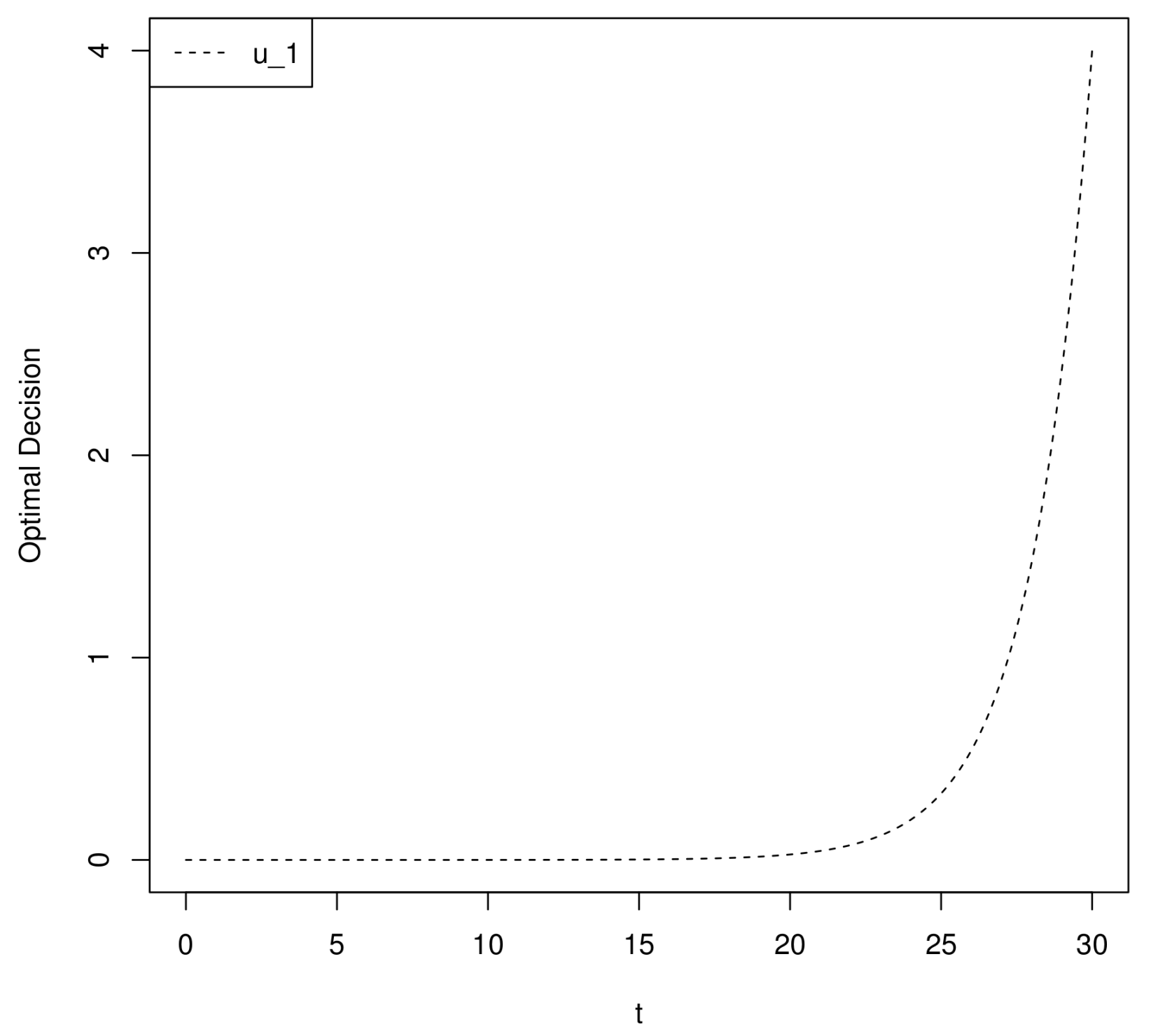
Figure 2 shows the time-varying optimal weight of $u_1^B$, from which we can see that ${u_1^B}^{*}$ increases exponentially with time t (with ${\nabla }_R^B=-0.5$, ${\lambda }_R=-0.5$, ${\lambda }_P=0.5$, $\gamma =0.5$ and $b=0.5$).

5. Sensitivity Analysis

In this section, we make a sensitivity analysis to show the relationship between optimal investment strategies and some parameters in Section 3. Unless otherwise stated, values of parameters in Section 5 and Section 6 are as follows: ${\nabla }_R^B=-0.5$, ${\lambda }_R=-0.5$, ${\lambda }_P=0.5$, $\gamma =0.5$, $b=0.5$, $t=0$ and $T=30$.

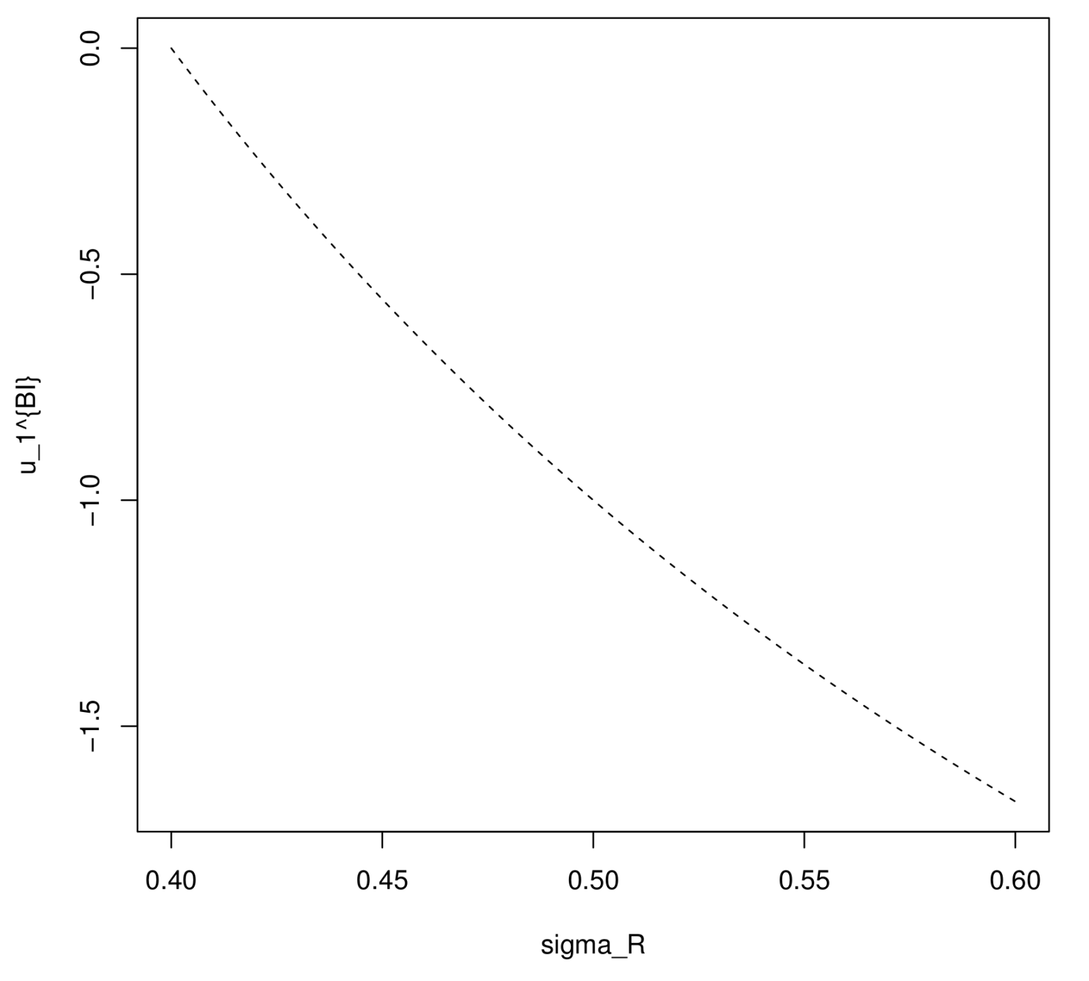
Figure 3 gives the relationship between the volatility and the optimal weight of the ordinary zero coupon bond. With suitable parameters chosen, the sponsor holds a short position of the ordinary bond. The optimal investment decision at initial time ${u_1^{BI}}^{*}(0)$ becomes lower, equivalently, the absolute value of ${u_1^{BI}}^{*}(0)$ becomes higher with a higher ${\sigma }_R$. It means that the ordinary bond becomes more attractive (even in a short position) when the value of ${\sigma }_R$ increases, since the premium of the ordinary bond ${\nabla }_R^B{\sigma }_R{\lambda }_R$ increases with a rising ${\sigma }_R$.

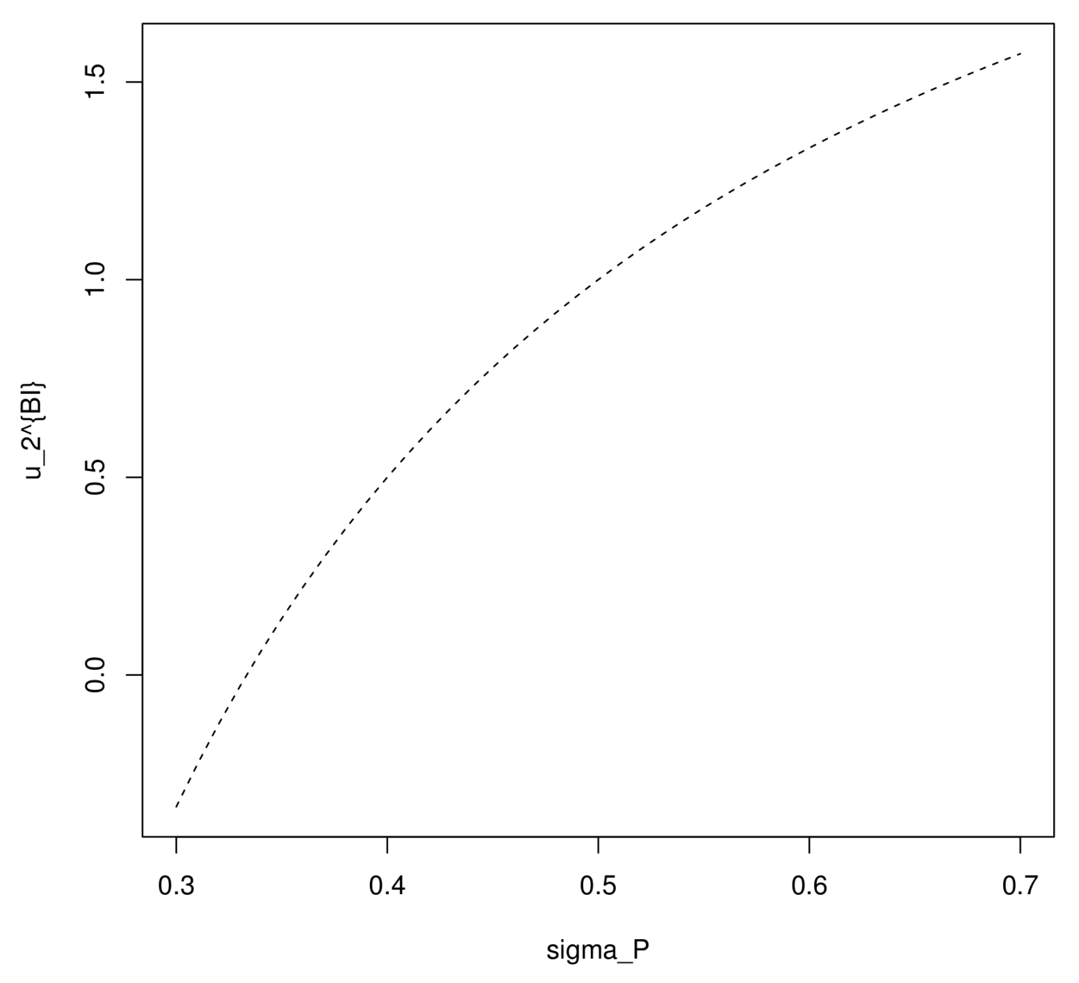
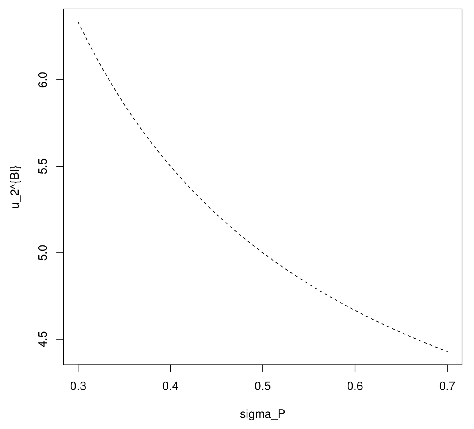
Figure 4 and Figure 5 show the relationship between the volatility and the optimal weight of the inflation-indexed bond, with positive ${\lambda }_P(=0.5)$ and negative ${\lambda }_P(=-0.5)$, respectively. In the case ${\lambda }_P=0.5$, the optimal investment strategy at initial time ${u_2^{BI}}^{*}(0)$ becomes higher with an increasing volatility ${\sigma }_P$, since the premium of the indexed bond ${\sigma }_P{\lambda }_P$ becomes higher, which means that the indexed bond becomes more attractive to investors. However, in the case ${\lambda }_P=-0.5$, the premium ${\sigma }_P{\lambda }_P$ decreases with a rising ${\sigma }_P$, which makes the indexed bond less attractive, so ${u_2^{BI}}^{*}(0)$ decreases with ${\sigma }_P$.

6. Comparative Statics and Conclusions

In order to investigate whether the inflation-indexed bond has an significant influence to the investment efficiency, a comparison between Section 3 and Section 4 is shown in the following theorem:

Theorem 3.

Set $t=0$. We have $V^{BI}(0,R,x)\ge V^B(0,R,x)$, which means that the maximum expected utility of the real terminal wealth by investing in an inflation-indexed bond is higher than that of a portfolio only consisting of an ordinary zero coupon bond and a money market account.

Proof. 

$$\begin{array}{ccc}\hfill {\alpha }^{BI}-{\alpha }^B& =& {\displaystyle \frac{1}{2}}{\displaystyle \frac{1-\gamma }{\gamma }}{({\lambda }_P-{\sigma }_P)}^2+{\displaystyle \frac{1}{2}}\gamma (1-\gamma ){\sigma }_P^2+(1-\gamma ){\sigma }_P({\lambda }_P-{\sigma }_P)\hfill \\ \hfill & =& {\displaystyle \frac{1}{2}}{\displaystyle \frac{1-\gamma }{\gamma }}{\left((1-\gamma ){\sigma }_P-{\lambda }_P\right)}^2\ge 0\hfill \end{array}$$

(36)

We have ${\alpha }^{BI}\ge {\alpha }^B$, thus $A_1^{BI}\ge A_1^B$, and the result follows. ☐

Remark 4.

From the first equation in (36), we have a higher $V^{BI}/V^B$ with a higher ${\lambda }_P-{\sigma }_P$. A rational explanation might be as follows: Since ${\lambda }_P=\frac{i-{\sigma }_P}{{\sigma }_P}$, ${\lambda }_P>{\sigma }_P$ is equivalent to $i>{{\sigma }_P}^2+{\sigma }_P$, i.e., when the expected inflation rate is significantly low, there is no remarkable advantage to invest in the inflation-indexed bond. Probably we can conclude that the hedging is not significant.

Now we investigate the influence of the difference between ${\lambda }_p$ and ${\sigma }_p$ to value functions. It is clear that in Figure 6, when ${\lambda }_p$ is greater than ${\sigma }_p$, the ratio between the value function corresponding the optimal problem with inflation-indexed bond and the value function corresponding the optimal problem without the indexed bond is almost increasing exponentially with the increasing of ${\lambda }_p-{\sigma }_p$. When we change the value of ${\sigma }_p$ to 0.48 and 0.46, it is easy to conclude that the curve increasing faster with ${\sigma }_p$ becomes smaller.

Remark 5.

The impact of terminal time T: In Figure 7, the ratio between two value functions again increasing exponentially with the increasing of the terminal time. A rational explanation of this phenomenon is that the investment becomes riskier with a longer time interval, and the hedging becomes more necessary by an indexed bond.

We make a conclusion as follows: This paper considers, by means of dynamic programming approach, the optimal investment strategy for the decumulative phase in DC type pension schemes under inflation environment. The objective is to determine the investment strategy, maximizing the expected CRRA utility of the terminal real wealth in a complete market consisting of an inflation-indexed bond, a zero coupon bond and a riskless asset. The explicit solution of the optimal problem is derived from the corresponding HJB equation. In order to investigate the role of the indexed bond, we also solve another optimal investment problem in an incomplete market with the indexed bond excluded. With any level of parameters, we find that the value function in the complete market is never lower than the value function in the incomplete market, i.e., the maximum expected utility of the terminal wealth by investing in an inflation-indexed bond is never lower than that of a portfolio without the index bond, thus we may conclude that an indexed bond definitely has significant advantage to hedge inflation risk.