Article

Modelling and Forecasting Stock Price Movements with Serially Dependent Determinants

by
Rasika Yatigammana
1,
Shelton Peiris
2,3,
Richard Gerlach
4 and
David Edmund Allen
2,5,6,*
1
Central Bank of Sri-Lanka, Colombo 01, Sri Lanka
2
School of Mathematics and Statistics, The University of Sydney, Sydney 2006, Australia
3
Department of Statistics, The University of Colombo, Colombo 03, Sri-Lanka
4
Discipline of Business Analytics, The University of Sydney, Sydney 2006, Australia
5
Department of Finance, Asia University, Taichung 41354, Taiwan
6
School of Business and Law, Edith Cowan University, Joondalup 6027, Australia
*
Author to whom correspondence should be addressed.
Risks 2018, 6(2), 52; https://doi.org/10.3390/risks6020052
Submission received: 16 March 2018 / Revised: 25 April 2018 / Accepted: 1 May 2018 / Published: 7 May 2018
(This article belongs to the Special Issue Computational Methods for Risk Management in Economics and Finance)

Abstract

:
The direction of price movements are analysed under an ordered probit framework, recognising the importance of accounting for discreteness in price changes. By extending the work of Hausman et al. (1972) and Yang and Parwada (2012),This paper focuses on improving the forecast performance of the model while infusing a more practical perspective by enhancing flexibility. This is achieved by extending the existing framework to generate short term multi period ahead forecasts for better decision making, whilst considering the serial dependence structure. This approach enhances the flexibility and adaptability of the model to future price changes, particularly targeting risk minimisation. Empirical evidence is provided, based on seven stocks listed on the Australian Securities Exchange (ASX). The prediction success varies between 78 and 91 per cent for in-sample and out-of-sample forecasts for both the short term and long term.

1. Introduction

There has been a significant growth in market micro-structure research, which is concerned with the study of the underlying process that translates the latent demands of investors into transaction prices and volumes (Madhavan 2000). The study of the time series properties of security prices has been central to market micro-structure research for many years. Madhavan (2000) asserts that frictions and departures from symmetric information do affect the trading process. Furthermore, insights into future price trends provides additional information useful in strategy formulation. As per financial economic theory, the asset returns cannot be easily predicted by employing statistical or other techniques and incorporating publicly available information. Nevertheless, recent literature bears evidence of successful forecasting of asset return signs; see for example, Breen et al. (1989); Leung et al. (2000); White (2000); Pesaran and Timmermann (2004) and Cheung et al. (2005). While having mean independence, it is statistically probable to have sign and volatility dependence in asset returns (Christoffersen and Diebold 2006).
The knowledge of the future direction of the stock price movement provides valuable guidance in developing profitable trading strategies. However, there is no clear consensus on the stochastic behaviour of prices or on the major factors determining the change in prices. In this context, theories of information asymmetry stating that private information deduced from trading causes market price fluctuations (See Kyle 1985) became important propositions. Consequently, many market attributes have been employed as substitutes for information in the study of security price behaviour. Price changes occur in discrete increments, which are denoted in multiples of ticks. It is well recognised today that failing to treat the price process as a discrete series could adversely affect prediction results. Initially the modeling of discrete transaction prices was done by Gottlieb and Kalay (1985). The generalisation and variation of such a modeling framework can be found in Ball (1988); Glosten and Harris (1988); Harris (1990); Dravid (1991) and Hasbrouck (1999). Most often, earlier studies have treated price change as a continuous variable, primarily focusing on the unconditional distribution, ignoring the timing of transactions, which is irregular and random. The “ordered probit model”, which was initially proposed by Aitchison and Silvey (1957) is a useful model for discrete dependent variables, which can take only a finite number of values with a natural ordering. Gurland et al. (1960) developed it further and later it was introduced into the social sciences by McKelvey and Zavoina (1975), which became an analytical tool in the financial market security price dynamics of micro-structure research. This could be used to quantify the effects of various factors on stock price movements, whilst accounting for discreteness in price changes and the irregular spacing of trades.
In an ordered probit analysis of the conditional distribution of price changes, Hausman et al. (1972) recognised the importance of accounting for discreteness, especially in intraday price movements. In such fine samples, the extent of price change is limited to a few distinct values, which may not be well approximated by a continuous state space. Their paper investigated the impact of several explanatory variables in capturing the transaction price changes. Importantly, the clock-time effect, measured in terms of duration between two consecutive trades, bid-ask spread, trade size and market-wide or systematic movements in prices based on a market index on conditional distribution of price changes were modeled under this framework. In a more recent study, Yang and Parwada (2012) extended the existing empirical literature on the impact of market attributes on price dynamics, utilising an ordered probit model. Their study explored the price impact of variables such as market depth and trade imbalance (also referred to as order imbalance in quote driven markets), in addition to trade size, trade indicator, bid-ask spread and duration which were found to be significant in similar studies. The model thus estimated by Yang and Parwada (2012), was able to forecast the direction of price change for about 72% of the cases, on average.
The in-sample and out-of-sample forecasts provided by the authors were based on the observed values of the regressors in the forecast horizon. However, in generating out-of-sample forecasts beyond one-step ahead incorporating observed values for regressors is of limited practical use, as they are not observed priori. Developing multi-step ahead forecasts, at least for a few transactions ahead is much more beneficial from a practical perspective, for effective decision making. However, such forecasting evidence under this framework is seemingly absent in the literature. Therefore, in addressing this shortcoming, this paper introduces a forecasting mechanism to generate forecasts beyond the one-step ahead level. Towards this end, disaggregated forecasts are generated first, for each of the explanatory variables for the period concerned. In order to generate forecasts for the regressors included, the serial dependence structure of each of the variables is investigated and appropriate forecasting models are fitted. Sign forecasts are subsequently generated, based on those predicted regressor values, rather than on observed values and the estimated coefficients of the ordered probit model. These prediction results are compared with those of the existing literature. Through the introduction of dynamic variables into the forecasting system, the predictive capability of this approach is investigated through a study based on the stocks of seven major companies listed in the Australian Securities Exchange (ASX).
In summary, the primary motivation of this paper is to introduce a method to enhance the flexibility and adaptability of the ordered probit model to generate multi-step ahead forecasts of stock price changes. Identifying and estimating appropriate univariate models for forecasting each explanatory variable, taking their serial dependence structure into account, towards this endeavour, is the second motivation. The third motivation is to improve on the results of Yang and Parwada (2012) in model estimation and forecast accuracy, by reducing noise in the data used and suitably formulating variables. Therefore, this exercise features the same stocks and almost the same independent variables that were employed by Yang and Parwada (2012). We were able to achieve an 88 per cent plus rate of accuracy, on average, in the out of-sample forecasts of the direction of price changes using observed regressor values. In addition, more than 91 per cent of in-sample estimates, on average, correctly predicted the direction of price change. This is in comparison to the 72 per cent achieved by Yang and Parwada (2012). It is between 78-80 per cent when predictied regressor values were incorporated.
The remainder of the paper is organized as follows. Section 2 provides a review of the ordered probit model while Section 3 gives a description of the data and the variables used in the analysis. This section reports the summary statistics for each variable for the chosen stocks and introduces the relevant models for estimation and forecasting of durations, residuals and regressors. The empirical evidence is reported in Section 4 including model estimation and diagnostics. The results of the forecasting exercise for both in-sample and out-of-sample are presented in Section 5 and finally, the concluding remarks are provided in Section 6.

2. A Review of the Ordered Probit Model

In a sequence of transaction prices, P t 0 , P t 1 , P t 2 , …, P t T occurring at times t 0 , t 1 , t 2 , …, t T the resulting price changes multiplied by 100 is represented as an integer multiple of a tick and denoted by Y 1 , Y 2 , …, Y T , where Y k { P t k P t k 1 } × 100 . The ordered probit model analyses discrete dependent variables with responses that are ordinal but not continuous. Underlying the indexing in such models, there exists a latent continuous metric and the thresholds partition the real line into a series of different regions corresponding to these ordinal categories. Therefore, the unobserved latent continuous variable Y * is related to the observed discrete variable Y. It is assumed that the conditional mean of Y * is described as a linear combination of observed explanatory variables, X and a disturbance term that has a Normal distribution.
The ordered probit specification takes the following form:
Y k * = X k β + ε k , where ε k | X k i . n . i . d . N ( 0 , σ k 2 ) ,
where i.n.i.d denotes that the errors are independently but not identically distributed. X k is a q × 1 vector of predetermined explanatory variables that govern the conditional mean, Y k * and β is a q × 1 vector of parameters to be estimated. Here, the subscript denotes the transaction time. The observed price change Y k is related to the latent continuous variable Y k * according to the following scheme:
Y k = s 1 if   Y k * A 1 s 2 if   Y k * A 2 s m if   Y k * A m ,
where the sets A k are comprised of non overlapping ranges of values, partitioning the continuous state space of Y k * and the s j are the corresponding discrete values containing the state space of Y k , which are called states. Let s j ’s be the price change in ticks −2, −1, 0, 1, …. Suppose that the threshold values of A are given as follows:
A 1 ( , α 1 ] , A 2 ( α 1 , α 2 ] , A k ( α k 1 , α k ] , A m ( α m 1 , ) .
The number of states, m is kept finite, though in reality price change could take any value in cents to avoid the explosion of an unknown number of parameters. As per Hausman et al. (1972), the only requirement in this framework is the conditional independence of the ε k ’s, where all the serial dependence would be captured by the regressors. Further, there are no restrictions on the temporal dependence of the X k ’s. The conditional distribution of Y k , conditioned upon X k depends on the partition boundaries and the distributional assumption of ε k . The conditional distribution in the case of Gaussian ε k is
P ( Y k = s i | X k ) = P ( X k β + ε k A i | X k )
= P ( X k β + ε k α 1 | X k ) if   i = 1 , P ( α i 1 < X k β + ε k α i | X k ) if   1 < i < m , P ( α m 1 < X k β + ε k | X k ) if   i = m ,
= Φ α 1 X k β σ k if   i = 1 , Φ α i X k β σ k Φ α i 1 X k β σ k if   1 < i < m , 1 Φ α m 1 X k β σ k if   i = m ,
where Φ ( · ) denotes the standard Normal cumulative distribution function. Since the distance between the conditional mean X k β and the partition boundaries determines the probability of any observed price change, the probabilities of attaining each state, given the conditional mean, could be changed by shifting the partition boundaries appropriately. The explanatory variables capture the marginal effects of various economic factors that influence the likelihood of a given state as opposed to another. Therefore, the ordered probit model determines the empirical relation between the unobservable continuous state space and the observed discrete state space as a function of the explanatory variables, X k , by estimating all the system parameters, including β coefficients, the conditional variance σ k 2 and the partition boundaries α , from the data itself.
Let U i k be an indicator variable, which takes the value 1 if the realisation of the kth observation, Y k is the ith state s i and 0 otherwise. The log likelihood function L for the price changes Y = [ Y 1 , Y 2 , , Y T ] , conditional on the regressors, X = [ X 1 , X 2 , , X T ] , takes the following form:
L ( Y | X ) = k = 1 T U 1 k . l o g Φ α 1 X k β σ k + i = 2 m 1 U i k . l o g Φ α i X k β σ k Φ α i 1 X k β σ k + U m k . l o g 1 Φ α m 1 X k β σ k
Hausman et al. (1972) has reparameterised the conditional variance σ k 2 based on the time between trades and lagged spread.

Models for Correlated Errors and Explanatory Variables

As mentioned in the above subsection, models with an appropriate autoregressive structure are used as forecasting models for the explanatory variables. Autoregressive integrated moving average (ARIMA) models of order (p,d,q) or ARIMA (p,d,q) models are used tomodel the autocorrelation in a time series and are used to predict behaviour based on past values alone. However, certain variables warranted the application of a simple ARIMA type model while others exhibit long range dependence, which require autoregressive fractionally integrated moving average (ARFIMA) (p,d,q) type models to describe their behaviour. On the other hand, forecasts of indicator variables with more than two categories are based on multinomial logistic regressions, where the responses are nominal categories. The heteroscedasticity in the residuals is captured by the generalised autoregressive conditional heteroscedasticity GARCH( p , q ) model (Bollerslev 1986), following (Yang and Parwada 2012). A brief description of each of these models are given in the Appendix.

3. Data, Variables and ACD Model

3.1. Data Description and ACD Model

The relevant data for this analysis was obtained from the Securities Industry Research Centre of Asia-Pacific (SIRCA) in Australia. The dataset consists of time stamped tick-by-tick trades, to the nearest millisecond and other information pertaining to trades and quotes for the chosen stocks listed in the Australian Securities Exchange (ASX). This study is based on a sample of stock prices collected during a three month period from 16 January 2014 to 15 April 2014. The stocks that were not subjected to any significant structural change, representing seven major industry sectors, are included in the sample. The selected stocks are Australian Gas Light Company (AGL), BHP Billiton (BHP), Commonwealth Bank (CBA), News Corporation (NCP), Telstra (TLS), Westfarmers (WES) and Woodside Petroleum (WPL) from Utilities, Materials, Financials, Consumer Discretionary, Telecommunication services, Consumer Staples and Energy sectors respectively. All seven of these stocks are included in the study by Yang and Parwada (2012), consisting of both liquid and less liquid assets, to minimise sample selection biases. However, the sampling period and the sample size differ between studies. Two stocks are not included in this paper due to the absence of transactions during the study period. Intraday price changes extracted from tick by tick trade data forms the basic time series under consideration. Overnight price changes are excluded as their properties differ significantly from those of intraday price changes (See Amihud and Mendelson 1987; Stoll and Whaley 1990). The trading hours of ASX are from 10.00 a.m. to 4.00 p.m. Due to the possibility of contamination of the trading process by including opening and closing trades (Engle and Russell 1998), the trades during the initial 30 min of opening and the final 30 min prior to closing are disregarded.
The following information with respect to each transaction is collected for each stock: Trade data comprising of date, time, transaction price and trade size, quote data such as bid price and ask price, market depth data comprising of volume at the highest bid price (best bid) and volume at the lowest ask price (best ask) and market index (ASX200). HFD generally contains erroneous transactions and outliers that do not correspond to plausible market activity. This is mainly attributed to the high velocity of transactions (Falkenberry 2002). Among others Hansen and Lunde (2006); Brownlees and Gallo (2006) and Barndorff-Nielsen et al. (2009) have paid special attention to the importance of data cleaning. A rigorous cleaning procedure is used here in obtaining a reliable data series for the analysis, mainly in accordance with the procedure outlined in Barndorff-Nielsen et al. (2009). To generate a time series at unique time points, during the instances of simultaneous multiple trades (quotes), the median transaction price (bid/ask prices) of those trades (quotes) is considered. Correspondingly, cumulative volume of those trades (quotes) are taken as the trade volume (bid/ask volume).
In the ordered probit model, the dependent variable Y k is the price change between the k th and k 1th trade multiplied by 100. This records Y k in cents, which however is equivalent to ticks as the tick size of the ASX for stocks with prices of the chosen magnitude is 1 cent. In this analysis, several different explanatory variables are included to measure their association with direction of price movement, following Yang and Parwada (2012). Bid and ask quotes are reported as and when quotes are updated, which necessitates the matching of quotes to transaction prices. Each transaction price is matched to the quote reported immediately prior to that transaction. Similarly, aggregate volumes at the best bid and best ask prices together with the ASX200 index representing the market are also matched in a similar fashion. The bid-ask spread S p r d k 1 , is given in cents, while L B A V k 1 & L B B V k 1 denote the natural log of number of shares at best ask and bid prices respectively. L V o l k 1 gives the natural logarithm of ( k 1 ) th trade size. Conditional duration, ψ k 1 and standardised transaction duration ϵ k 1 are derived estimates by fitting an autoregressive conditional duration model (ACD (1,1)) to diurnally adjusted duration data. A brief description of the model introduced by Engle and Russell (1998) is presented in Appendix A. The initial record of each day is disregarded as it is linked to the previous day’s prices and results in negative durations. T I k 1 denotes the trade indicator of ( k 1 ) th trade, which classifies a trade as buyer-initiated, seller-initiated or other type of trade. Trade imbalance T I B k 1 , based on the preceding 30 trades that occurred on the same day (Yang and Parwada 2012) (YP hereafter) is calculated as follows:
T I B k 1 = j = 1 30 T I ( k 1 ) j × V o l ( k 1 ) j j = 1 30 V o l ( k 1 ) j
The first 30 observations of trade imbalance (TIB) is set to zero as TIB also depends on the previous day’s trade imbalance for these transactions.
Market index return R I n d x k 1 , prevailing immediately prior to transaction k is computed as given below:
R I n d x k 1 = ln ( I N D X k 1 ) ln ( I N D X k 2 )
The sampling period and the use and categorisation of certain variables in this analysis differ from YP. ASX200 is applied here instead of specific sector indexes as the impact of the performance of the overall economy tends to be more significant on stock price behaviour than of a specific sector. On the other hand, the reference point for grouping the price changes is the ‘one tick’ threshold vis a vis the ‘zero’ change. This provides a more meaningful classification of the groups, as the categorisation of price change is based on a range of values rather than a fixed value for a certain group.

3.2. Sample Statistics

The main characteristics of the chosen variables in the analysis and how those characteristics differ between stocks could be ascertained from the several summary statistics that are provided in Table 1. There is considerable variation in the price level among the stocks considered in the sample. The highest price during this period ranged between AUD 4.96 for TLS and AUD 77.87 for CBA. The volatility of prices as indicated by the standard deviation of the percentage price change is not very high, with the TLS recording the highest value of 7.65 per cent. For most other stocks, it is less than 5 per cent. Average trade volume also records a substantial dispersion between the stocks, which varied from 161 for NCP and 6983 for TLS during the period. An indication of whether a transaction is buyer-initiated or seller-initiated is required for the empirical analysis. This measure is useful in identifying the party most anxious to execute the trade and the actions of whom would be reflected in terms of the bid/ask spread. The trades fall into these two categories in more or less equal proportions across stocks and are very similar in value except for TLS. The indeterminate trades form around 8–18% of trades, while it is 45% for TLS. The absence of asymmetric pressure from the buying or selling side suggests that there were no events with major news impact that would have resulted in abnormal trades and returns. This is further highlighted by zero mean returns.
The trading frequency as measured by the average duration between two consecutive trades also varies across stocks significantly. For more liquid stocks such as BHP, CBA and WES, trades tend to occur every 5 s or less on average. The other stocks are generally traded within 10 s. However, NCP is traded every 25 s on average. The observed large dispersions is a characteristic inherent in trade durations. Next, the estimation of the duration dynamics under an ACD model is considered, since the expected and standardised durations enter the orderd probit model as two separate variables.
The estimated coefficients of the ACD (1,1) model fitted to diurnally adjusted durations is presented in Table 2. The multiplicative error component is assumed to follow a Standardised Weibull distribution. All the coefficients are highly significant for each of the stocks, indicating the dependence of the expected duration on its past behaviour. It is straightforward to estimate the conditional expected durations, ψ k utilising the parameter estimates from the ACD model. The diurnal component was estimated using a cubic spline with knots at each half hour between 10:30 a.m. and 15:30 p.m. The standardised durations or the unexpected durations, ϵ k are then obtained by dividing the diurnally adjusted durations by the conditional expected durations, which is an i.i.d. process. The parameter estimates are based on the conditional maximum likelihood approach, using the standardised Weibull distribution for ϵ k . The Weibull distribution is a better choice here as opposed to exponential since the shape parameter is statistically significant and different from unity for all the stocks. Refer to the Appendix for the corresponding log-likelihood function.
The standardised durations are deemed weakly exogenous in the case of Australian stocks, according to the regression results of YP. They have regressed the standardised residuals on trades, volumes and returns for each of the stocks, which included the seven stocks of our study. On the other hand, both these studies consider the lagged measures of duration, addressing the problem of endogeneity to some extent. Furthermore, Dufour and Engle (2000) have treated durations as a strongly exogeneous variable in assessing the role of time on price dynamics.
The volumes at the best bid and ask prices prevailing prior to a transaction gives a measure of market depth. TLS has the deepest market, minimising the price impact cost for its trades. The trade imbalance (TIB) attempts to capture the cumulative demand side and supply side discrepancy over the last 30 trades. TIB < 0, if seller-initiated cumulative trading volume exceeded the buyer-initiated cumulative trading volume, during the immediately preceeding 30 trades prior to the current transaction. On the other hand, TIB > 0, if the buyer-initiated volume was more than the seller-initiated volume. The zero indicates either all indeterminate trades or an exact matching of selling and buying volumes during the period. In any case, zeros are very rare. Overall, there is a insignificant trade imbalance across all stocks. However, three stocks have a negative sign implying the selling volume marginally exceeded the buying volume while the other four stocks have a positive sign indicating the reverse phenomenon.
It is noticed that most of the variables exhibit serial correlation, with variables such as L V o l , L B B V , L B A V , S p r d , T I and T I B showing strong serial dependence, for all stocks. For illustration, Figure 1, Figure 2 and Figure 3 present the time series behaviour together with the acf and pacf for a few selected variables for a random stock, AGL.
A novel feature of this study is that unlike in YP’s study, we incorporate this feature by developing forecasting models for each explanatory variable based on the serial dependence structure. Therefore, Section 2.1 reports some useful models for capturing this feature in X k ’s and σ k 2 , while details of the forecasting exercise is discussed later in Section 5.1.

4. Empirical Evidence

The model estimation for the direction of price change is carried out for these stocks for the period 16 January to 14 April 2014. Out of sample forecasts are generated for the last day of the sample, on 15 April 2014 from 10:30 a.m. to 15:30 p.m.
Y k denotes the price changes between the k and ( k 1 ) th trades in terms of integer multiples of ticks. The price change here is representative of the change in the observed transaction prices. The number of states that could be assumed by the observed price changes Y k 
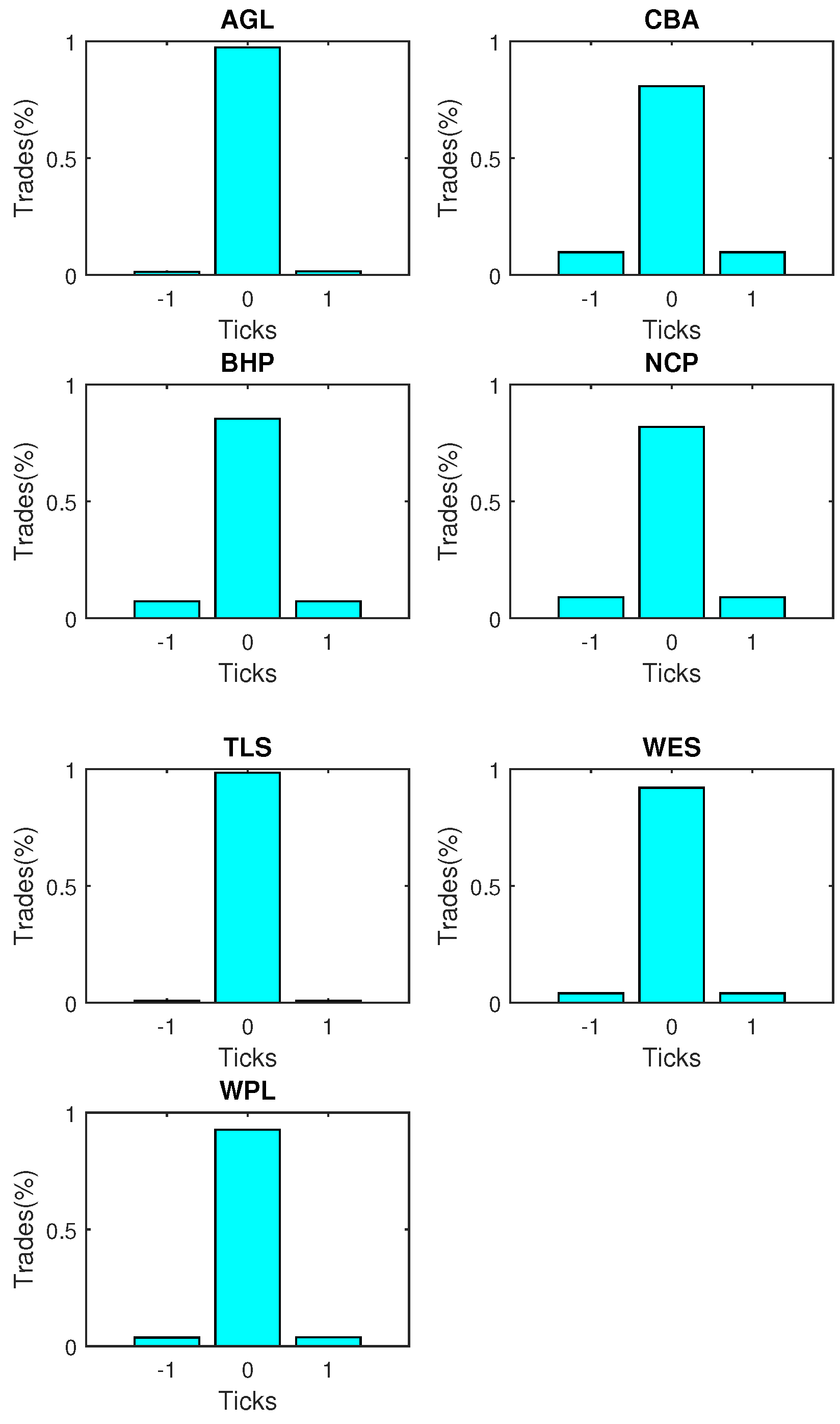
is set to 3, under the ordered probit framework. Price increases of at least 1 tick being grouped as +1, price decreases of at least 1 tick as −1, while price changes falling in (−1,1), taking the value 0. The choice of m is based on achieving the balance between price resolution and minimising states with zero or very few observations. The decision to restrict m to 3 was mainly influenced by the fact that the observed price changes exceeding ± 2 ticks was below 0 . 05 % for most stocks. The distribution of observed price changes in terms of ticks, over the transactions, is presented in Figure 4. Prices tend to remain stable in more than 80 per cent of the transactions, in general. For the rest of the time, rises and falls are more or less equally likely.

4.1. Ordered Probit Model Estimation

Prior to model estimation, all variables considered in the analysis was tested for stationarity using an Augmented Dickey-Fuller (ADF) test, which confirmed the same, which is in agreement with previous findings. The Ordered probit model specification depends on the underlying distribution of the price series. The model can assume any suitable arbitrary multinomial distribution, by shifting the partition boundaries accordingly. However, the assumption of Gaussianity here has no major impact in deriving the state probabilities, though it is relatively easier to capture conditional heteroscedasticity.
The dependent variable in Equation (11) below is the price change in ticks. (An explanation of the latent continuous version of the price change was given in Section 2). The variables used in Equation (11) were described in Section 3. Just to recap, the first three variables on the R.H.S. of Equation (11) are three lags of the dependent variable. T I k 1 is the trade indicator; which classifies a trade as a buyer-initiated, seller-initiated or other type of trade. S P R D k 1 , 
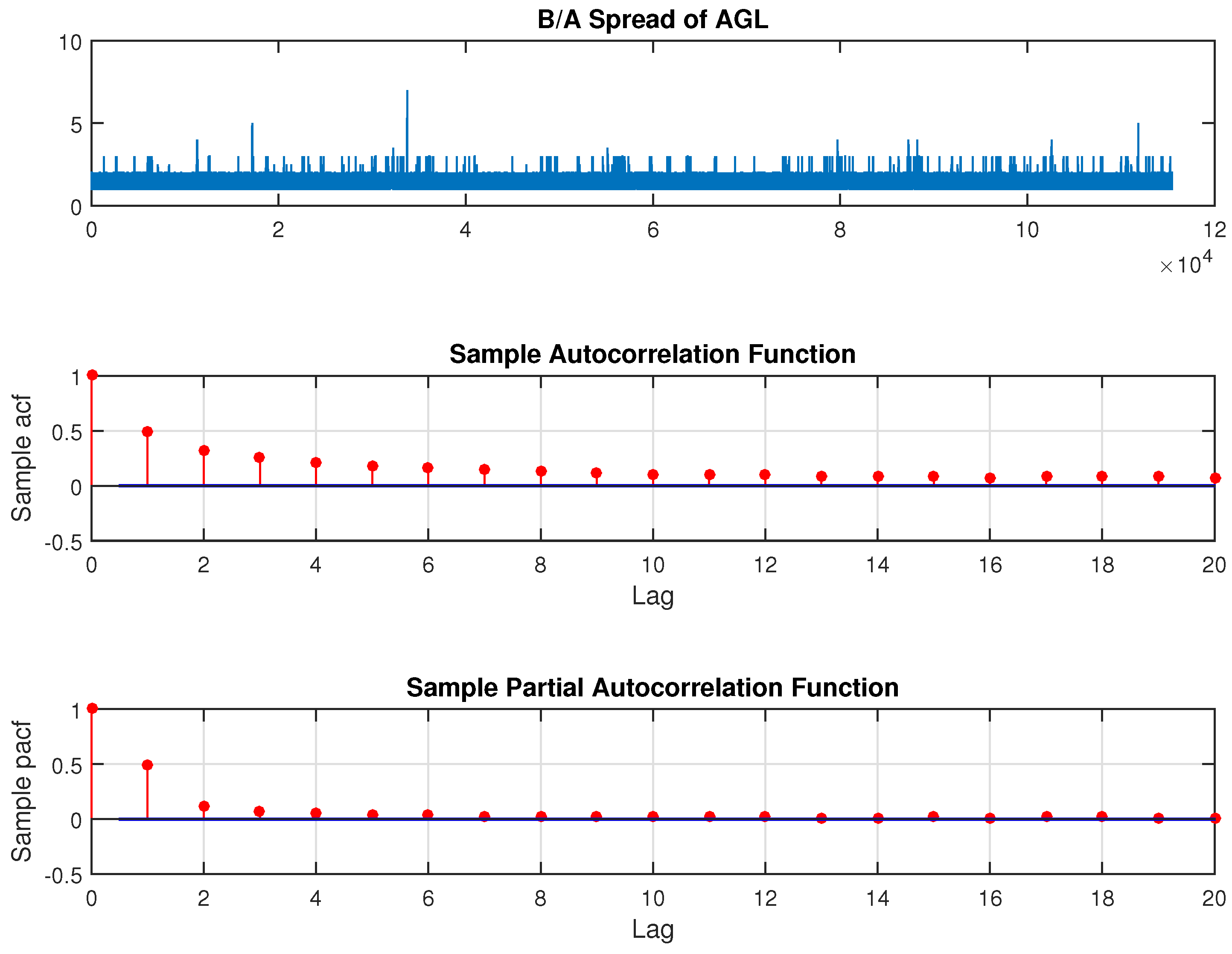
is the Bid-Ask spread, measured in cents. L V o l k 1 gives the natural logarithm of ( k 1 ) th trade size. L B A V k 1 and L B A B V denote the natural log of number of shares at best ask and bid prices respectively. T I B k 1 is the trade imbalance, based on the preceding 30 trades on the same day. Conditional duration, ψ k 1 and standardised transaction duration ϵ k 1 are derived estimates by fitting an autoregressive conditional duration model (ACD (1,1)) to diurnally adjusted duration data. The ACD (1,1) model is described in the appendix. R I n d x k 1 , prevailing immediately prior to transaction k, is calculated as the continuously compounded return on the ASX 200.
The mean equation under the ordered probit specification takes the following form:
X k β = β 1 Y k 1 + β 2 Y k 2 + β 3 Y k 3 + β 4 T I k 1 + β 5 S p r d k 1 + β 6 L V o l k 1 + β 7 L B A V k 1 + β 8 L B B V k 1 + β 9 T I B k 1 + β 10 T I k 1 ψ k 1 + β 11 T I k 1 ϵ k 1 + β 12 R I n d x k 1
The maximum likelihood estimates of the ordered probit model on price changes were computed based on BHHH algorithm of Berndt et al. (1974). The estimated coefficients of the above ordered probit system are presented in Table 3 while the corresponding z statistics are recorded within parentheses. Most of the regressors are highly significant to the model for all seven stocks, based on the asymptotically normally distributed z statistic (Hausman et al. 1972). The pseudo- R 2 values given at the bottom of the table show an improvement, irrespective of the number of observations, in comparison to those of YP. A relatively higher number of significant coefficients across all stocks is another improvement.
The first three lags of the dependent variable comes under scrutiny, first. All the lags are significant with a 95% confidence level, with a negative coefficient for each stock. This inverse relationship with past price changes is consistent with the existing literature, indicating a reversal in the price compared to its past changes. Consider a one tick rise in price over the last three trades in the case of AGL, for example, keeping the other variables constant. The subsequent fall in the conditional mean ( Y k * ) would be 3.9448, which is less than the lower threshold, resulting in −1 for Y k . The coefficients of the traditional variables such as the bid ask spread ( S p r d ), trade volume (LVol) and the market index returns are significant for all stocks but one, in each case. The S p r d and L V o l has a positive impact on the price change across all stocks. The market index returns, based on the ASX200, as a measure of the overall economy, generally has a significant positive impact on price changes. Overall, this is in line with the conventional wisdom. Meanwhile, the coefficients of the trade indicator, the number of shares at the best bid price and the number of shares at the best ask price are significant for all stocks.
The trade imbalance ( T I B ) between buyers and sellers has a positive impact on price change and is statistically significant across all stocks. This phenomenon agrees well with the general inference that more buyer-initiated trades tend to exert pressure from the demand-side, resulting in a subsequent rise in price and vice versa. The impact of the time duration between trades is measured separately via the two constituent components of an ACD model. One is the conditional expected duration (signed), T I k 1 ψ k 1 and the other isthe standardised innovations (signed), also referred to as unexpected durations, T I k 1 ϵ k 1 . The signed conditional expected duration is significant for all stocks while the unexpected component is significant for all but one. This highlights the informational impact of time between trades in price formation. The interpretation of these measures of duration is not straightforward as they are comprised of two components. The kind of impact those variables have on price change will depend on the significance of the trade initiation as well as on the durations. One striking feature is that either both the components have a positive impact or both have a negative impact for a given stock. Wald tests were performed to investigate the significance of duration on price changes. The tests were conducted under the null hypotheses in which either the coefficient of the conditional duration is zero or the coefficient of standardised duration is zero or both are jointly zero. The resultant F statistics suggest that both the components of duration are significant for all the stocks considered. The test results are not presented here for the sake of brevity.
The partition boundaries produced below the coefficient estimates determine the partition points of the direction of change in the latent variable. There are three possible directions the price change can take in terms of ticks, Y k 1 , Y k = 0 and Y k + 1 . By comparing these boundary values with the estimated continuous variable Y k * , values −1, 0 or +1 are assigned to the observed variable Y ^ k .
In parameterising the conditional variance, an ARMA specification was used following YP. Therefore, a GARCH ( p , q ) specification including up to two lags was used on the residual series of the ordered probit model across all stocks. The orders p , q were selected on the basis of Akaike information criterion (AIC). The selected parameter estimates of the fitted GARCH models are reported in Table 4. Only some of the parameters appear to be significant with less persistence in conditional volatility for some stocks.

4.2. Price Impact of a Trade

Price impact measures the effect of a current trade of a given volume on the conditional distribution of the subsequent price movement. In order to derive this, X k β has to be conditioned on trade size and other relevant explanatory variables. The volumes, durations and the spread were kept at their median values while the index was fixed at 0.001 whereas trade indicator and trade imbalance were kept at zero to minimise any bias. It is observed that the coefficients of the three lags of Y k are not identical, implying path dependence of the conditional distribution of price changes (Hausman et al. 1972). Consequently, the conditioning has to be based on a particular sequence of price changes as well, as a change in the order will affect the final result. These conditioning values of X k ’s specify the market conditions under which the price impact is to be evaluated.
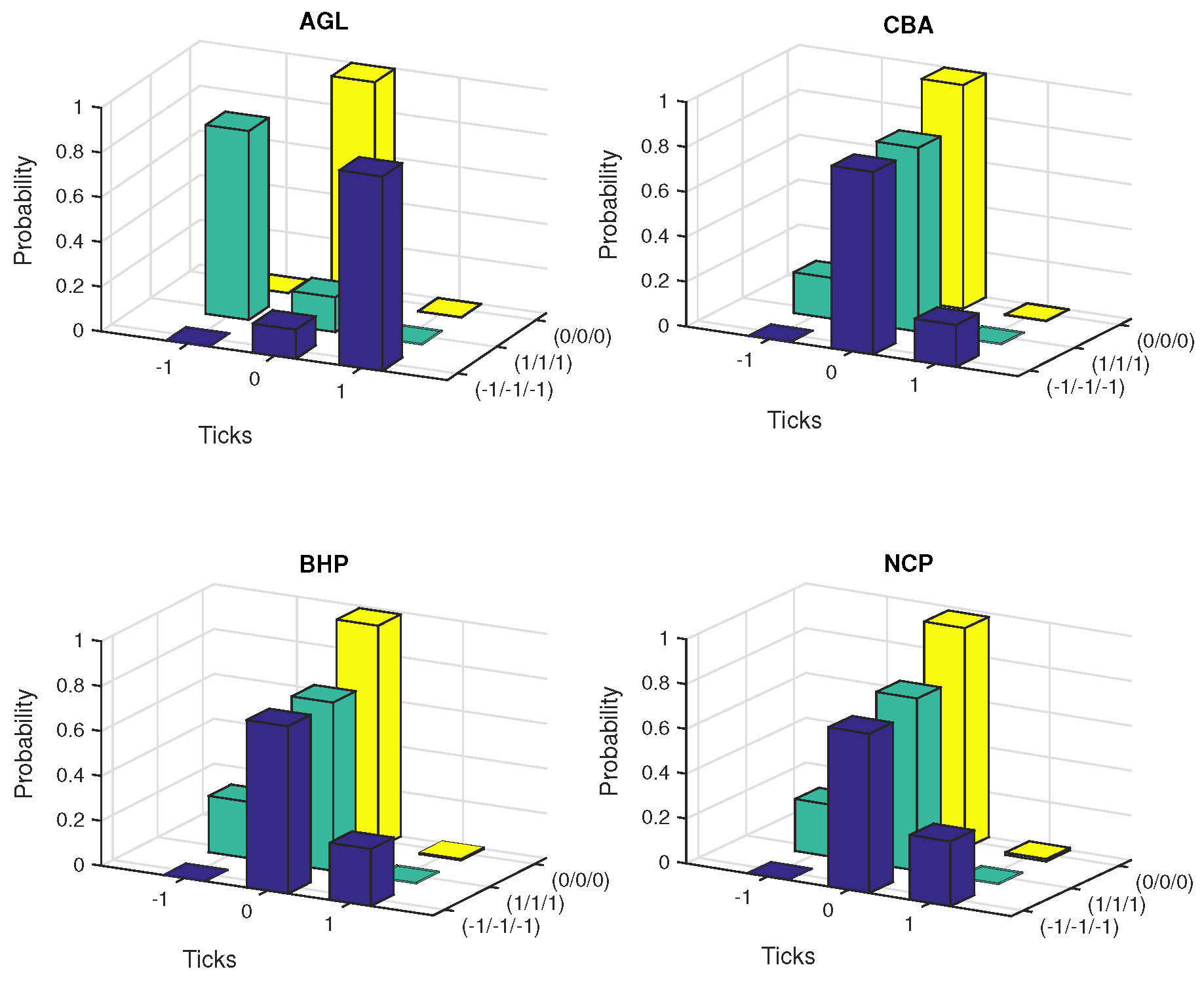
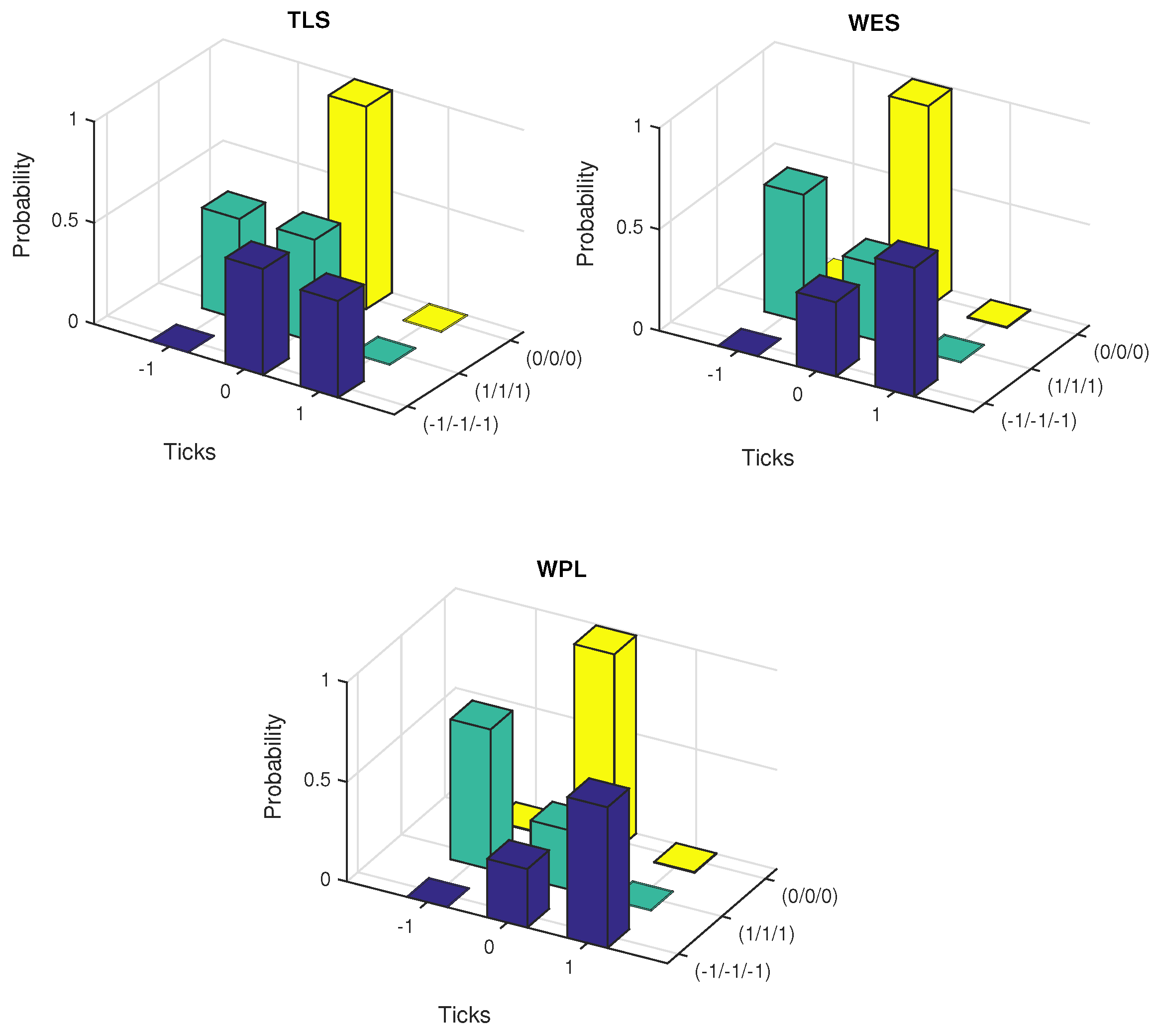
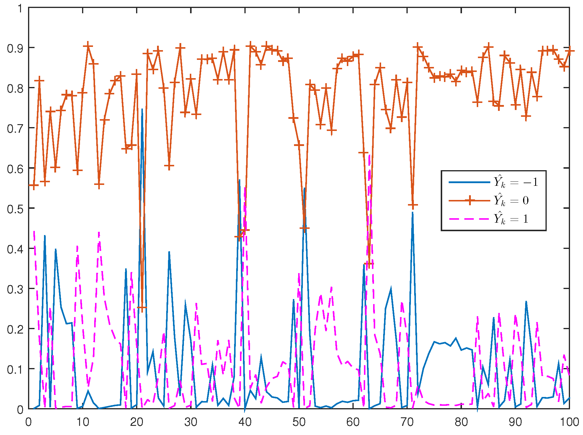
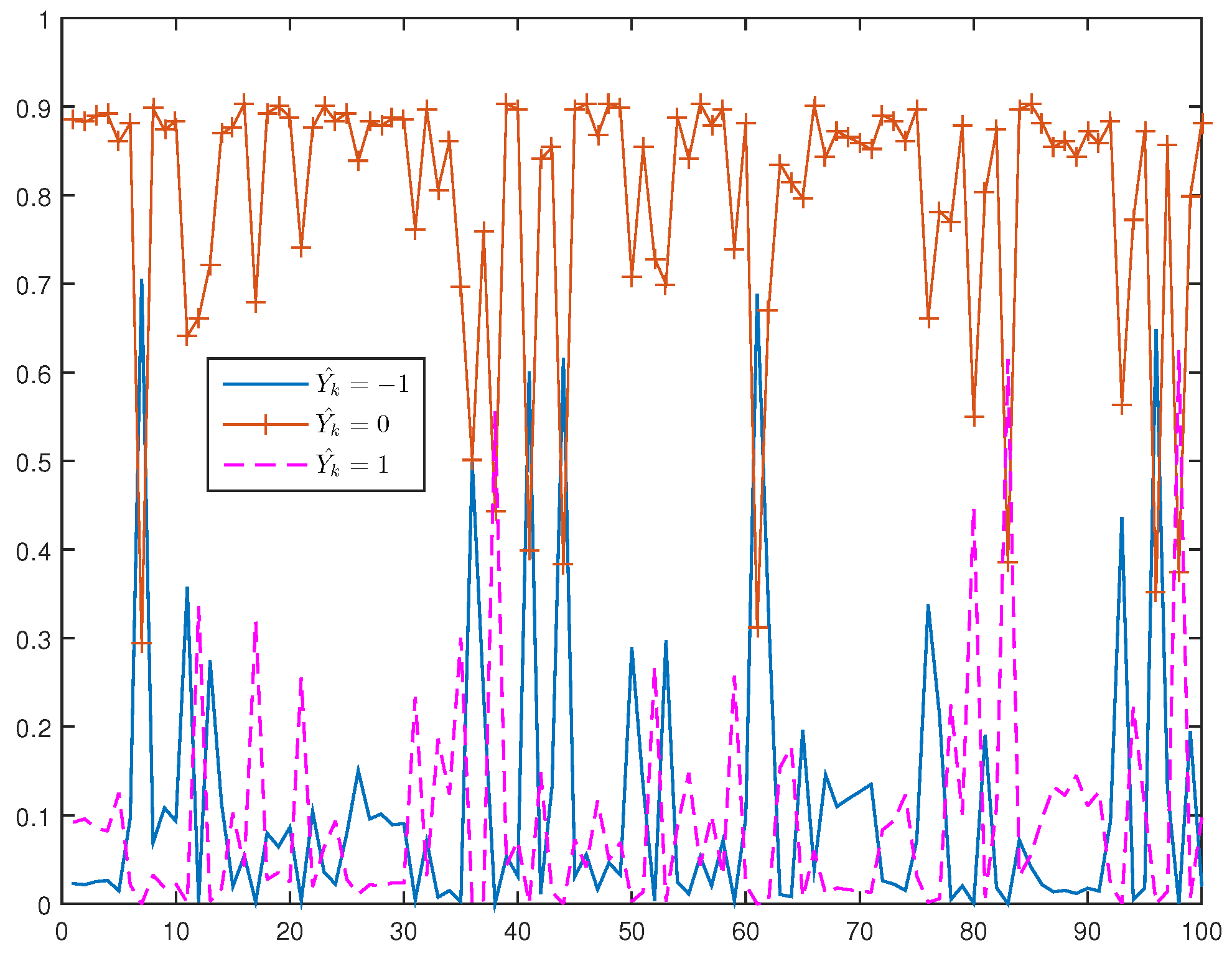
The conditional probabilities were estimated under five scenarios of path dependence keeping the other quantities at the specified values. These are falling prices (−1/−1/−1), rising prices (1/1/1), constant prices (0/0/0) and alternative price changes, (−1/+1/−1) and (+1/−1/+1). Figure 5 and Figure 6 exhibit the plots of estimated probabilities under the first three scenarios for all the seven stocks. The shifts in the distribution are clearly evident for the first two cases as against the third case of constant prices. Under the falling price scenario, the shift is more towards the right while for the rising price scenario, it is more towards the left indicating an increased chance of price reversal after three consecutive rises or falls. In the case of alternating prices it was revealed that prices tend to remain stable in the subsequent trade.

4.3. Diagnostics

A well specified ordinary least squares (OLS) regression would exhibit little serial correlation in the residuals. A similar kind of test could be performed on the generalised residuals in the case of ordered probit to test its validity, as it is not possible to obtain residuals directly (Hausman et al. 1972). Table 5 contains the sample cross-correlation coefficients of generalised residuals with the lagged generalised fitted values, Y ^ k j , computed up to 12 lags. Under the null hypothesis of no serial correlation, the theoretical cross-correlation coefficients should be zero or close to zero. The reported values are quite small, varying in the range from −0.01 to 6.19 × 10 6 .

5. Forecasting the Direction of Price Change

The forecasting performance of the ordered probit model fitted to the stocks is investigated. The tests of in-sample and out of-sample forecasts provide some basis to gauge the model’s ability to accurately forecast the future direction of price changes. Forecasts are generated under three scenarios. In-sample probability estimates are based on the last week of the training sample from 8 April to 14 April 2014. Meanwhile, out-of-sample forecasts are based on the final day of the data series, 15 April. Only one day is considered for the out-of-sample performance as it is not feasible to project price changes beyond one day with any degree of accuracy as a normal trading day contains more than 1000 transactions for all the stocks, with the exception of NCP which had only 417. Out-of-sample forecasts are computed in two ways. One is one-step ahead forecasts based on the observed, recorded values of the regressors and the other is the multi-step ahead, using their predicted values. The next subsection discusses the forecast generation under the second scenario in more detail. The commonly observed measures of forecast performance are not so relevant in this case, since the dependent variable is categorical. However, some measures such as root mean square error (RMSE) and mean absolute deviation (MAD) were calculated for both in-sample and out-of-sample forecasts, though they are not reported here for the sake of brevity.

5.1. Out-of-Sample Multi-Step Ahead Forecasts with Disaggregated Predictions of Individual Explanatory Variables

In real life, the values of the regressors are not observed priori, to forecast at least a few transactions ahead. Unlike in YP’s study this paper develops out-of-sample multi-step ahead forecasts based on disaggregated predictions of the regressors. Under this scenario, multi-step ahead forecasts are generated for the entire forecast horizon, based on the estimated models, as well as 100-step ahead rolling basis. The rolling forecasts of price change are based on similar forecasts of explanatory variables. Towards this end, we first predict the future values of the regressors based on models that are fitted to capture the autoregressive behaviour of each variable in the sample. Under this setup, forecasts of price change are derived for the estimated transactions occurring on the last day of the series, 15 April 2014. The relevant models are fitted after a careful inspection of the autocorrelation function (acf) and the partial autocorrelation function (pacf) of the individual series, as discussed in Section 2.1. The model selection among several competing models is based on the AIC for a given regressor. In most instances, the time series of L V o l shows a hyperbolic decay in their acfs and pacfs, similar to Figure 1. Therefore, an ARFIMA type model is the preferred choice for L V o l . The fractional differencing parameter, d is always within the range of 0 to 0.5, indicating the presence of long memory. On the other hand, most other variables such as L B B V , L B A V , T I B and S p r d have slow decaying autocorrelations and partial autocorrelations, with the majority falling short of a hyperbola. Figure 2 gives a general perception on the behaviour observed in these variables. For these regressors, an ARMA type model suffices for most stocks, in general. Forecasts of trade indicator are based on a multinomial logistic regression on L B A V , L B B V , lags of Y and lags of T I , as the common contenders for the explanatory variables. Parameter estimates of predictive models for selected variables are illustrated in Table 6 and Table 7 for the stock, AGL. The expected and unexpected durations are forecasted by the estimated ACD model.

5.2. Forecast Performance of the Ordered Probit Model

The basic test of forecast errors is mainly based on the number of correct forecasts as a percentage of total forecasts. The fitted directions of price change, Y ^ k , based on the estimated coefficients are compared with their actual counterparts for each transaction in the forecasting sample. The number of exact tallies provide the number of correct forecasts. The in-sample forecast results illustrated in Table 8 reports a 91% accuracy, which is a very high percentage, by any means, vouching for the significant forecasting ability of the model. In comparison, YP achieved a percentage of 72. On the other hand, out-of sample results are provided in Table 9. For one-step ahead forecasts based on observed regressor values, the direction could be accurately predicted 88 per cent of the time, on average, across all stocks. The percentage achieved by YP again is 72 per cent. Meanwhile, the performance of the multi-step ahead forecasts based on the fitted regressor values is not as striking as in the other two cases, as expected. Notwithstanding, percentages of 78 and 85, on average, are highly noteworthy and are still higher than the 72 per cent of YP. The comparatively dismal performance of TLS under the first scenario given in panel 2 (a) of Table 9 may have been influenced by a relatively small number of price changes recorded during the period. However, the rolling forecasts show a remarkable improvement. The ex-post forecast of this stock is slightly better than the ex-ante forecast, which is quite contrary to the other stocks. The reverse is observed for five of the other stocks, as anticipated, while for one stock, it is similar.
The predictions of regressors based on serial correlation structures do not provide very good long term multi-step ahead forecasts, due to mean reversion. As a result of this, the forecasts of price change direction, based on those fitted values may also not provide reliable long term forecasts. A single day is referred to as longterm as the average daily transactions exceed 1000 for most stocks in the sample. Therefore, under these circumstances, the forecast horizon is restricted to the 100 transactions of the last day on a rolling basis, which resulted in a much better accuracy percentage of 85, in comparison to the one incorporating all the transactions of that day. It is worthwhile mentioning that from an individual stock’s perspective, the short term performance is better than the long term. The worst case scenario gives around 75 per cent of out-of-sample correct forecasts, whereas it is around 85 per cent for the in-sample predictions.
Based on predicted price movements, investors can adjust their trading positions accordingly in formulating trading strategies, risk management, portfolio allocations etc. However, the most risky position under these forecast scenarios would be the adverse selection (see Yang and Parwada 2012, for more details). It is where the actual occurrence is the opposite of the predicted price movement, with possible adverse effects on the investor’s networth. Therefore, it is worthwhile examining the extent of the possibility of this risk of adverse selection taking place. The percentages of predictions in the opposite direction for actual rise/fall are given in Table 8 and Table 9 for in-sample predictions and out-of-sample forecasts respectively. Generally, this risk is very small and not more than 1 per cent across all stocks, except TLS, under all the forecast scenarios. In the case of out-of-sample forecasts, TLS records a 50 per cent risk of adverse selection, mainly as a result of only two recorded price falls in the forecast sample. Furthermore, altogether there are only three rises/falls in the price, giving rise to zero correct classifications for those categories for TLS.
The predicted conditional probabilities of the three categories of forecast price change Y ^ k , −1, 0 and 1 are generated under the ordered probit system for in-sample as well as out-of-sample forecasts. Y ^ k is assigned the value of the category with the highest probability for a given transaction. These probabilities obtained for the stock, CBA, are illustrated for 100 observations during the forecast period, in Figure 7 and Figure 8 to represent all the stocks, which show similar behaviour. For a given observation, the vertical sum of the three conditional probabilities is one. In the case of both in-sample and out-of-sample scenarios, the probabilities tend to fluctuate. However, for the majority of observations, no price change category tends to have a probability greater than 50 per cent, in general, resulting in lower percentages of correct classifications for rises and falls in prices. This does not indicate a deviation from the real life behavior in prices, with respect to the overall distribution across the three categories. Nevertheless, this phenomenon highlights a slight over prediction in that category. A similar pattern of behaviour is observed for the forecasts with predicted regressors as well.
As discussed earlier, most of the trades do not witness heavy movements in prices. Nevertheless, if a rise/fall in price could be foreseen in advance, investors are in a better position to create profitable strategies or to manage risk appropriately. Since multi-step ahead predictions of opposite price movements are rare, a forecast rise/fall would provide useful signals of future price directions. This, when combined with the knowledge of past price paths, will aid the investor in making a more informed decision in strategy formulation in his favour, especially towards minimising risk. However, improving the individual forecasts of the explanatory variables will be beneficial in realising better predictions of future price movements under this framework.

6. Conclusions

The future direction of stock price movements are predicted through the estimation of an ordered probit model under an empirical setup. The study comprises of intra-day transaction data of seven stocks representing seven industry sectors, listed on the ASX. The ordered probit specification seems to adequately capture the price changes. All the explanatory variables are highly significant for the majority of the stocks. Diagnostics indicate lack of serial correlation in residuals with the implication of the model providing a good fit. The sequence of trades has an impact on the conditional distribution of price changes, while the trade size too is important with larger volumes putting more pressure on prices.
In improving forecast accuracy of the model, our study differs from that of YP in certain respects. Percentage of success in predicting future direction of price movements is used as a yardstick to measure the forecasting strength of the model. The success rate of the in-sample predictions is around 91 per cent and out-of sample one-step ahead forecasts happens to be 88 per cent. These percentages are much higher than the respective percentage of 72 per cent achieved by YP, for both cases. Overall, our forecasts outperform those of YP for each common stock.
Another main contribution of this study is to forecast price changes within a more practical perspective. In real life, the values of the regressors are not known a-priori to forecast at least a few transactions ahead. In addressing this drawback, we first predict the future values of the regressors based on their serial correlation structures by way of appropriate models. This resulted in several Autoregressive Moving Average (ARMA) and Autoregressive Fractionally Integrated Moving Average (ARFIMA) type models. In a subsequent step, these disaggregated forecasts are incorporated into the ordered probit model to generate future price change forecasts. Obviously, the 100-steps ahead short term forecasts perform better than the longterm ones including all transactions in the forecast horizon for most stocks. On average, the successful percentage in the long term is still a reasonable 78 per cent, which is affected by a poorly performing stock. On the other hand, the average success rate in the short term is around 85 per cent, which is quite remarkable.
Given the considerably high percentage of constant prices in real life, the model captures this phenomenon, albeit with a slight bias towards predicting no change. However, the risk of adverse selection is minimised. Nevertheless, this predictive model is useful for investors in developing successful trading strategies, particularly towards minimising risk as this provides valuable signals towards the future directions of price movements. The usefulness of this model to growth driven investors could be enhanced by improving the forecasting accuracy of the independent variables by adopting more sophisticated econometric techniques within a unified framework. In addition, the investigation of the adequacy of the conditional variance specification may also prove useful in improving the forecast probabilities.

Author Contributions

R.Y., R.G., S.P. and D.E.A. conceived and designed the experiments. R.Y. performed the experiments and analysed the data. R.Y., R.G., S.P. and D.E.A. wrote the paper.

Acknowledgments

The authors thank the reviewers for helpful comments.

Conflicts of Interest

The authors declare no conflict of interest.

Appendix A. Models for Errors and Explanatory Variables

Appendix A.1. ACD Specification to Model Transaction Durations

The Autoregressive Conditional Duration (ACD) model analyses transaction duration, identifying it as a conditional point process.The temporal dependence of the diurnally adjusted duration process is captured by the conditional expected duration, ψ k = E ( x k | x k 1 , , x 1 ) , under a linear ACD( p , q ) specification and has the following form:
ψ k = α 0 + i = 1 p α i x k i + j = 1 q β j ψ k j ,
where p 0 ; q 0 . The standardized durations
ϵ k = x k ψ k
are i.i.d. with E ( ϵ i ) = 1 . The log likelihood function for the Std. Weibull errors, is
L ( x | θ ) = k = 2 T α ln Γ 1 + 1 α + ln α x k + α ln x k ψ k Γ 1 + 1 α x k ψ k α ,
where α is the shape parameter of the density.

Appendix A.2. GARCH Specification to Model Heteroscedasticity

Conditional variance in the residuals ( ε k ) of the orderd probit model, σ k 2 can be estimated from this model.
ε k = σ k η k , ε k | X k ( o , σ k 2 )
where σ k 2 is the conditional volatility of ε k given the past historical information, η k is a sequence of independently and identically distributed (i.i.d.) random variables with zero mean and variance 1 such that
σ k 2 = ω + i = 1 p κ i σ k i 2 + j = 1 q δ j ε k j 2 .

Appendix A.3. ARIMA Model

A series { X k } that could be modeled as a stationary ARMA( p , q ) process after being differenced d times is denoted as ARIMA( p , d , q ) with the following form:
ϕ ( B ) ( 1 B ) d X k = c + θ ( B ) a k ,
where ϕ ( B ) = 1 ϕ 1 ϕ p , θ ( B ) = 1 + θ 1 + + θ q and a k W N ( 0 , σ a 2 ) and B is the backshift operator.

Appendix A.4. Long Memory ARFIMA Model

ARFIMA is designed to capture the long range dependence in time series. This model extends the ARIMA model in (A3) allowing d to lie between −0.5 and + 0.5 yielding a fractionally integrated series. ARFIMA process is said to exhibit stationary long memory if d ( 0 , 0 . 5 ) . See Granger and Joyeux (1980) for details.
An ARFIMA( p , d , q ) process has the same form as in (A3) and the operator ( 1 B ) d is given by
( 1 B ) d = k = 0 Γ ( k d ) B k Γ ( d ) Γ ( k + 1 ) ; d { 1 , 2 , }

Appendix A.5. Multinomial Logistic Regression

Multinomial logistic regression is an extension of binary logistic regression, that handles polytomous responses. This is used to predict the response category or the probability of category membership of a nominal outcome variable. The log odds of the outcome are modeled as a linear combination of multiple explanatory variables.
If x k = ( x k 1 , x k 2 , , x k r ) follows a multinomial distribution with r response categories and parameter π k = ( π k 1 , π k 2 , , π k r ) , then
l o g π k j π k j * = y k T β j , j j *
considering j * as the baseline category. Assuming that m th category is the baseline category ( j * = m ) , the coefficient vector is
β = ( β 1 , β 2 , . . . , β m 1 , β m + 1 , . . . , β r )

References

  1. Aitchison, John, and Samuel D. Silvey. 1957. The generalization of probit analysis to the case of multiple responses. Biometrika 44: 131–40. [Google Scholar] [CrossRef]
  2. Amihud, Yakov, and Haim Mendelson. 1987. Trading mechanisms and stock returns: An empirical investigation. The Journal of Finance 42: 533–53. [Google Scholar] [CrossRef]
  3. Ball, Clifford A. 1988. Estimation bias induced by discrete security prices. The Journal of Finance 43: 841–65. [Google Scholar] [CrossRef]
  4. Barndorff-Nielsen, Ole E., P. Reinhard Hansen, Asger Lunde, and Neil Shephard. 2009. Realized kernels in practice: Trades and quotes. The Econometrics Journal 12: C1–32. [Google Scholar] [CrossRef]
  5. Berndt, Ernst R., Bronwyn H. Hall, Robert E. Hall, and Jerry A. Hausman. 1974. Estimation and inference in nonlinear structural models. Annals of Economic and Social Measurement 3: 653–65. [Google Scholar]
  6. Bollerslev, Tim. 1986. Generalized autoregressive conditional heteroskedasticity. Journal of Econometrics 31: 307–27. [Google Scholar] [CrossRef]
  7. Breen, William, Lawrence R. Glosten, and Ravi Jagannathan. 1989. Economic significance of predictable variations in stock index returns. Journal of Finance 44: 1177–89. [Google Scholar] [CrossRef]
  8. Brownlees, Christian T., and Giampiero M. Gallo. 2006. Financial econometric analysis at ultra-high frequency: Data handling concerns. Computational Statistics & Data Analysis 51: 2232–45. [Google Scholar]
  9. Cheung, Yin-Wong, Menzie D. Chinn, and Antonio Garcia Pascual. 2005. Empirical exchange rate models of the nineties: Are any fit to survive? Journal of International Money and Finance 24: 1150–75. [Google Scholar] [CrossRef]
  10. Christoffersen, Peter F., and Francis X. Diebold. 2006. Financial asset returns, direction-of-change forecasting, and volatility dynamics. Management Science 52: 1273–87. [Google Scholar] [CrossRef]
  11. Dravid, Ajay R. 1991. Effects of Bid-Ask Spreads and Price Discreteness on Stock Returns. Technical Report. Philadelphia: Wharton School Rodney L. White Center for Financial Research. [Google Scholar]
  12. Dufour, Alfonso, and Robert F. Engle. 2000. Time and the price impact of a trade. Journal of Finance 55: 2467–98. [Google Scholar] [CrossRef]
  13. Engle, Robert F., and Jeffrey R. Russell. 1998. Autoregressive conditional duration: A new model for irregularly spaced transaction data. Econometrica 66: 1127–62. [Google Scholar] [CrossRef]
  14. Falkenberry, Thomas N. 2002. High Frequency Data Filtering. Great Falls: Tick Data Inc. [Google Scholar]
  15. Glosten, Lawrence R., and Lawrence E. Harris. 1988. Estimating the components of the bid/ask spread. Journal of Financial Economics 21: 123–42. [Google Scholar] [CrossRef]
  16. Gottlieb, Gary, and Avner Kalay. 1985. Implications of the discreteness of observed stock prices. The Journal of Finance 40: 135–53. [Google Scholar] [CrossRef]
  17. Granger, Clive W. J., and Roselyne Joyeux. 1980. An introduction to long-memory time series models and fractional differencing. Journal of Time Series Analysis 1: 15–29. [Google Scholar] [CrossRef]
  18. Gurland, John, Ilbok Lee, and Paul A. Dahm. 1960. Polychotomous quantal response in biological assay. Biometrics 16: 382–98. [Google Scholar] [CrossRef]
  19. Hansen, Peter R., and Asger Lunde. 2006. Realized variance and market microstructure noise. Journal of Business & Economic Statistics 24: 127–61. [Google Scholar]
  20. Harris, Lawrence. 1990. Estimation of stock price variances and serial covariances from discrete observations. Journal of Financial and Quantitative Analysis 25: 291–306. [Google Scholar] [CrossRef]
  21. Hasbrouck, Joel. 1999. The dynamics of discrete bid and ask quotes. The Journal of Finance 54: 2109–42. [Google Scholar] [CrossRef]
  22. Hausman, Jerry A., Andrew W. Lo, and A. Craig MacKinlay. 1992. An ordered probit analysis of transaction stock prices. Journal of Financial Economics 31: 319–79. [Google Scholar] [CrossRef]
  23. Kyle, Albert S. 1985. Continuous auctions and insider trading. Econometrica: Journal of the Econometric Society 53: 1315–35. [Google Scholar] [CrossRef]
  24. Leung, Mark T., Hazem Daouk, and An-Sing Chen. 2000. Forecasting stock indices: A comparison of classification and level estimation models. International Journal of Forecasting 16: 173–90. [Google Scholar] [CrossRef]
  25. Madhavan, Ananth. 2000. Market microstructure: A survey. Journal of Financial Markets 3: 205–58. [Google Scholar] [CrossRef]
  26. McKelvey, Richard D., and William Zavoina. 1975. A statistical model for the analysis of ordinal level dependent variables. Journal of Mathematical Sociology 4: 103–20. [Google Scholar] [CrossRef]
  27. Pesaran, M. Hashem, and Allan Timmermann. 2004. How costly is it to ignore breaks when forecasting the direction of a time series? International Journal of Forecasting 20: 411–25. [Google Scholar] [CrossRef]
  28. Stoll, Hans R., and Robert E. Whaley. 1990. Stock market structure and volatility. Review of Financial Studies 3: 37–71. [Google Scholar] [CrossRef]
  29. White, Halbert. 2000. A reality check for data snooping. Econometrica 68: 1097–126. [Google Scholar] [CrossRef]
  30. Yang, Joey Wenling, and Jerry Parwada. 2012. Predicting stock price movements: An ordered probit analysis on the Australian Securities Exchange. Quantitative Finance 12: 791–804. [Google Scholar] [CrossRef]
Figure 1. Time series, acf and pacf for LVol of AGL.
Risks 06 00052 g001
Figure 2. Time series, acf and pacf for spread of AGL.
Risks 06 00052 g002
Figure 3. Time series, acf and pacf for trade indicator of AGL.
Risks 06 00052 g003
Figure 4. Distribution of the number of trades over the three categories of price change in terms of ticks, for all stocks during the period.
Risks 06 00052 g004
Figure 5. Distribution of estimated probabilities of direction of price change conditioned on constant, increasing and decreasing past price changes.
Risks 06 00052 g005
Figure 6. Distribution of estimated probabilities of direction of price change conditioned on constant, increasing and decreasing past price changes.
Risks 06 00052 g006
Figure 7. In-sample estimated probabilities of direction of price change for 100 observations of CBA.
Risks 06 00052 g007
Figure 8. Out of-sample estimated probabilities of direction of price change for 100 observations of CBA, based on actual regressor values.
Risks 06 00052 g008
Table 1. Descriptive statistics of the variables considered in the ordered probit model for all the stocks, for the period from 16 January 2014 to 15 April 2014.
StatisticAGLBHPCBANCPTLSWESWPL
Price (AUD)
Max price16.1539.7977.8720.175.2943.9339.5
Min price14.7135.0672.1516.924.9640.8836.54
Price Change (%)
Mean0.00000.00000.00000.00000.00000.00000.0000
Std.dev0.03760.01970.01240.07280.07650.01810.0183
Duration (Seconds)
Mean9.593.513.4924.768.044.265.30
Std.dev19.017.377.5649.9112.479.0811.08
Trade Volume
Mean3957102851616983281318
Std.dev22063622218371139,37913701290
Shares at the Best Bid Price
Mean445154981579877941,00218411983
Std.dev5027646428991994603,01525042406
Shares at the Best Ask Price
Mean439955131808977992,90619452100
Std.dev5409754450531649642,20427752719
Market Index Returns, ASX200
Mean0.00000.00000.00000.00000.00000.00000.0000
Std.dev0.00010.00010.00010.00010.00010.00010.0001
Trade Imbalance
Mean−0.0268−0.01190.0094−0.06230.00940.02240.0004
Std.dev0.46530.45900.44010.48630.50820.45640.4446
Trade Direction (%)
Buyer initiated40.941.044.743.927.044.244.6
Seller initiated41.641.042.248.127.640.641.9
Table 2. The coefficient estimates of an ACD (1,1) model with Standardised Weibull errors fitted for the stocks. The conditional expected duration where x k is the adjusted duration. α is the shape parameter of the Weibull distribution.
ParameterAGLBHPCBANCPTLSWESWPL
α 0 0.31770.00240.31780.03480.02910.33490.0030
(21.92 *)(10.16 *)(32.47 *)(10.03 *)(28.82 *)(23.33 *)(6.65 *)
α 1 0.31130.01100.21950.14760.21800.16520.0201
(27.91 *)(20.61 *)(41.03 *)(15.53 *)(59.84 *)(29.71 *)(18.48 *)
β 0.47640.98650.49490.85240.78200.52200.9785
(26.80 *)(1371.66 *)(40.08 *)(89.69 *)(214.64 *)(30.26 *)(747.16 *)
α 0.25230.42950.42580.43690.57560.41940.4046
(427.88 *)(726.73 *)(731.49 *)(255.94 *)(476.06 *)(672.39 *)(582.99 *)
* Significant at 99% level.
Table 3. Coefficient estimates β i , of ordered probit model on direction of price change based on 12 explanatory variables for the selected stocks. The sampling period was 16 January 2014 to 15 January 2014. Z statistics are given within parentheses for each parameter.
ParameterAGLBHPCBANCPTLSWESWPL
Obs.114,318316,547317,76141,085137,323260,954205,651
Y k 1 −2.2281−1.0240−0.7915−0.7637−1.7745−1.4750−1.6261
(−72.21 *)(−130.16 *)(−119.64 *)(−54.32 *)(−53.16 *)(−143.59 *)(−113.69 *)
Y k 2 −1.1262−0.3614−0.3247−0.2554−0.9070−0.7413−0.8578
(−37.38 *)(−50.67 *)(−52.35 *)(−18.92 *)(−21.15 *)(−72.42 *)(−62.50 *)
Y k 3 −0.5905−0.1142−0.1153−0.1405−0.4252−0.3533−0.4137
(−19.79 *)(−16.65 *)(−19.56 *)(−10.50 *)(−12.21 *)(−33.69 *)(−30.20 *)
T I 0.95721.2730−0.2832−0.1256−1.23190.88990.9831
(67.69 *)(285.32*)(−88.07 *)(−8.95 *)(−38.61 *)(165.00 *)(146.16 *)
S p r d 0.04790.03420.00780.01170.07030.02380.0261
(3.16 *)(6.71 *)(2.60 *)(1.85 **)(1.21)(0.95)(4.83 *)
L V o l 0.00470.00900.00500.01670.01180.00600.0043
(1.16)(6.13 *)(3.67 *)(4.92 *)(3.04 *)(3.03 *)(1.85 **)
L B A V 0.08010.10190.0337−0.0312−0.05150.03980.0607
(12.36 *)(48.39 *)(20.31 *)(−6.94 *)(−4.76 *)(15.25 *)(19.05 *)
L B B V −0.0760−0.1097−0.03970.02520.0425−0.0575−0.0744
(−12.03 *)(−53.04 *)(−23.81 *)(5.66 *)(3.32 *)(−21.15 *)(−21.51 *)
T I B 0.04880.06470.09290.04570.19160.09860.0696
(2.52 *)(9.70 *)(15.89 *)(3.04 *)(9.47 *)(11.50 *)(6.77 *)
T I ψ −0.2246−0.37640.73040.0353−0.0546−0.2506−0.2631
(−31.79 *)(−119.95 *)(203.38 *)(4.24 *)(−3.91 *)(−62.24 *)(−56.41 *)
T I ϵ −0.0535−0.06080.07060.0013−0.0213−0.0314−0.0328
(−11.51 *)(−37.49 *)(55.74 *)(0.40)(−4.01 *)(−14.58 *)(−12.73 *)
R I n d x 262.0988110.1514194.2312307.72−107.5324342.8466139.1455
(3.30 *)(2.47 *)(3.71 *)(7.49 *)(−0.87)(6.52 *)(2.72 *)
α 1 −2.8628−2.1469−1.6552−1.5723−4.5651−2.3399−2.4639
α 2 2.99992.18691.66991.76765.13752.24032.3768
Pseudo R 2 0.32030.33390.22260.20680.32230.25890.2833
* Significant at 95% level. ** Significant at 90% level.
Table 4. Coefficient estimates of GARCH parameters of the conditional variance of the residuals for all stocks. ω , constant; κ , GARCH parameters; δ , ARCH parameters
ParameterAGLBHPCBANCPTLSWESWPL
Obs.114,318316,547317,76141,085137,323260,954205,651
ω 0.40810.04680.00220.05980.02040.32420.3282
(0.3419)(0.5782)(0.4748)(0.3415)(0.1226)(0.5995)(0.4998)
κ 1 0.31940.38030.97230.82550.91750.24450.2406
(0.2182)(0.3205)(46.8638)(2.4207)(2.9561)(0.2668)(0.2209)
κ 2 0.5157 0.20450.2172
(0.4516) (0.2272)(0.2019)
δ 1 0.25230.04290.02440.08730.06150.17350.1660
(0.6870)(0.9682)(1.4103)(0.6766)(0.0.2994)(1.3347)(1.1188)
Table 5. Cross-autocorrelation coefficents v ^ j , j = 1 , , 12 of generalised residuals with lagged generalised fitted price changes.
ParameterAGLBHPCBANCPTLSWESWPL
v ^ 1 −0.0025−0.0002−0.0015−0.00040.0004−0.0015−0.0004
v ^ 2 −0.00570.0012−0.0015−0.0002−0.0012−0.00030.0009
v ^ 3 −0.0103−0.0005−0.00160.0008−0.00080.00100.0015
v ^ 4 −0.00586.19 × 10 6 −0.0018−0.0029−0.0028−0.00040.0013
v ^ 5 −0.00450.0006−0.0018−0.0022−0.00390.0005−0.0017
v ^ 6 −0.0056−0.0001−0.0020−0.00250.00160.00310.0018
v ^ 7 0.0009−0.0008−0.00180.0002−0.00150.00340.0001
v ^ 8 0.00290.0001−0.00170.0043−0.00390.00100.0003
v ^ 9 0.0001−7.76 × 10 5 −0.00170.0057−0.00230.0036−0.0023
v ^ 10 0.00470.0003−0.00150.0039−0.00210.00300.0042
v ^ 11 0.00760.0020−0.00130.0025−0.00330.00090.0017
v ^ 12 0.00110.0014−0.00110.0014−0.00410.0024−0.0002
Table 6. Coefficient estimates of autoregressive model parameters fitted to selected independent variables. The t statistics are given within parentheses. Illustrative examples include a long memory and a short memory model for L V o l and S p r d for the stock AGL. d , long memory parameter; ϕ , AR parameters; θ , MA parameters.
ParameterLVolSpread
(ARFIMA)(ARMA)
c 0.0030 (7.30)
d0.1867 (68.50)
ϕ 1 0.0082 (15.72)1.7555 (160.732)
ϕ 2 −0.7581 (−71.06)
θ 1 −0.0079 (−35.59)−1.3455 (−123.55)
θ 2 0.2774 (41.16)
θ 3 0.0621 (15.35)
θ 4 0.0136 (3.67)
θ 5 0.0052 (1.80)
Table 7. Coefficient estimates of multinomial logistic regression model parameters fitted to Trade indicator ( T I ) of AGL. The base category is 1. Z statistics are given in parentheses.
IndependentCategory
Variable−10
c0.1449 (2.63)−1.9155 (−26.87)
d p k 1 0.2095 (5.08)0.1128 (1.98)
l b b v k 1 −0.3146 (−60.57)−0.0746 (−10.41)
l b a v k 1 0.3001 (60.42)0.2302 (35.96)
T I k 1 −0.9664 (−119.26)−0.4632 (−42.96)
Table 8. In-sample predictions of direction of price change for the last one week period of the training sample from 8 April 2014 to 14 April 2014.
ParameterAGLBHPCBANCPTLSWESWPL
One Week—08/04–14/04
Observations 114,318316,547317,76141,085137,323260,954205,651
accuracy ( % ) 97.8086.2085.1185.2498.7592.1994.76
−140.0023.7936.0325.4839.2927.1138.45
099.7998.6798.1498.6499.6599.5199.78
+145.4024.2935.7332.0136.0033.5737.09
ActualForecastNo.%No.%No. %No. %No. %No. %No. %
−1+10010.0560.3210.420 00 00 0
+1−1000 030.170 00 00 00 0
Table 9. Out-of sample forecasts of direction of price change for the last day of the sample, 15 April 2014. First panel contains one-step ahead forecasts based on actual explanatory variables and the second panel, muti-step ahead with predicted variables.
ParameterAGLBHPCBANCPTLSWESWPL
One-Step Ahead—15/04
Observations 115133194073417121825183638
accuracy ( % ) 97.8385.9079.6575.3099.6788.2891.70
−135.2927.4026.8021.540.0032.5432.77
099.7398.4797.3196.8299.9298.9599.47
+138.8923.8426.8837.680.0038.0335.53
Actual ForecastNo. %No.%No. %No. %No. %No. %No. %
−1 +1000061.2000021.200
+1 −1000010.200000000
Multi-Step Ahead—15/04
(a) All transactions
Observations 115133194073417121825183638
accuracy ( % ) 97.7482.7474.9367.8747.4687.4190.07
(b) 100-step ahead
accuracy ( % ) 97.4883.2580.5574.8279.9789.8792.25
−130.7725.3421.9420.000.0023.7820.43
098.9394.9499.87100.0080.1699.1499.88
+138.4629.1823.7223.190.0027.4525.71
Actual ForecastNo.%No.%No.%No.%No.%No.%No.%
−1 +10020.6830.58001500000
+1 −100000000000000

