1. Introduction
The global financial crisis and, more recently, the European sovereign crisis, have led to an increasing research literature on systemic risk, with different definitions and measurement models. According to
ECB (
2009), “Systemic risk is the risk of experiencing a strong systemic event, which adversely affects a number of systemically important intermediaries or markets”. This definition introduces two key elements for the study of systemic risk: first, a strong (triggering) event, affecting the entire system as a whole and not only individual institutions; second, a correlation component between market participants that could result from contagion effects between financial institutions and the underlying system they are part of, or from the recursive spread of adverse effects from one financial institution or market to another one.
While systemic risk definitions share this broad view, systemic risk measurement models are still quite divergent. A first diversity concerns the economic environment as the context in which systemic risk arises and propagates. Many models concentrate on the financial sector while others deal only with the sovereign sector: the two, however, are strongly linked to each other. A second distinction derives from the use of a cross-sectional rather than a time-dynamic perspective: while the former mostly concentrates on contagion between the institutions operating in a given market, the latter focuses on the generating cause-and-effect relationships over time. In other words, if contagion models identify the transmission channels of risk, thus describing how a crisis spreads through the whole system, time-dependent models associate a specific risk measure to individual institutions, with the aim of predicting their level of risk in the nearby future by using an early-warning perspective. A third distinction originates in the identification of the risk sources, thus setting endogenous against exogenous causes, as well as idiosyncratic against systematic shocks.
In this work, we will develop a general measurement model that can be applied regardless of the above-mentioned classification. First, we will consider Credit Default Swap spreads as a measure of credit risk of the underlying institution. CDS spreads can refer to any institutions, whether they are sovereign countries, financial institutions or non financial corporates: therefore, there is no need to adopt different measurement models for each considered sector. Second, we will model CDS spreads by means of a class of Vector Auto Regressive models that can account for both temporal and cross-sectional dependency. Doing so, we will be able not only to describe the contagion transmission mechanisms, but also to construct early-warning predictive measures for the risk level of each single institution. We will thus derive a contagion risk variable, called , able to describe how many extra basis points should be paid to insure one monetary unit of credit when contagion effects deriving from other market participants are taken into account. Such form of contagion can be negative, thus causing the spread to increase (typical behaviour of “risk importer” countries), but also positive, thus determining the spread to decrease (typical behaviour of “risk exporter” countries). Third, the proposed VAR model will be able to disentangle the risk measure into two components regardless of the nature of the original shock (endogeneous or exogeneous, individual or systematic): one reflecting pure contagion mechanisms, the other one accounting for idiosyncratic risk.
To exemplify the methodology, the proposed model will be applied to the sovereign CDS spreads of ten countries. Five of them represent core countries: the United States, the United Kingdom, Japan, Germany and France. The other five are the European countries that most suffered from the recent sovereign crisis: Italy, Spain, Portugal, Ireland and Greece. First, our results based on correlation networks indicate that contagion induces a “clustering effect”: after an initial shock in the periphery, the risk measure of core and peripheral countries further diverges through, and because of, contagion propagation, thus creating a sort of diabolic loop within the sovereign sector. Second, our empirical findings based on the two disentangled components of risk show that the contagion effect, measured by , is extremely strong in euro area countries, and especially in the largest economies (Germany, France, Italy, Spain). The outcomes also show that peripheral countries mostly behave as exporters, rather than importers of system risk: as a consequence, core economies have been negatively affected by contagion risk in the last years, while the predominant risk component for peripheral countries still consists of higher idiosyncratic default probabilities. One notable exception is Greece, which is strongly affected by both contagion and idiosyncratic risks. Finally, from an interpretational viewpoint, the variable introduced in this study can be considered as a valid network centrality measure, while having clear advantages over classic measures since it is expressed in basis points rather than general real numbers difficult to benchmark.
The paper is structured as follows:
Section 2 contains the literature background necessary for the development of our research methodology, described in
Section 3;
Section 4 contains the main empirical findings from the application of the models, and
Section 5 concludes with some final remarks.
2. Background
From a chronological viewpoint, the first systemic risk measures have been proposed for the financial sector, in particular by
Adrian and Brunnermeier (
2016),
Acharya et al. (
2012,
2017) and
Brownlees and Engle (
2016). On the basis of market share prices, these models consider systemic risk as endogenously determined and calculate the quantiles of the estimated loss probability distribution of a financial institution, conditional on an extreme event in the financial market (or vice versa). The above approach is useful to establish policy thresholds aimed, in particular, at identifying the most systemic financial institutions, or the most systemic countries. However, it is designed as a bivariate approach: on one hand, this allows for calculating the risk of an institution conditional on a reference market; on the other hand, such approach does not address the issue of how risks are transmitted between different institutions in a multivariate framework.
A different stream of research considers systemic risks as exogenous and explains them by means of causal factors. This approach has been proposed, in particular, by
Ang and Longstaff (
2013),
Betz et al. (
2014),
Duprey et al. (
2015),
Schwaab et al. (
2016) and
Ramsay and Sarlin (
2016), who explain whether the default probability of a bank, of a country, or of a company depends on a set of exogenous risk sources, thus combining idiosyncratic and systematic factors. While powerful from an early warning perspective, causal models, similarly to bivariate ones, concentrate on single institutions rather than on the financial system as a whole and, therefore, may underestimate systemic sources of risk arising from contagion effects within the system.
To address systemic risks, correlation network models that combine financial networks (see, e.g.,
Lorenz et al. (
2009) and
Battiston et al. (
2012)) with contagion models based on the dependence structure among market prices have been proposed by
Billio et al. (
2012) and
Diebold and Yilmaz (
2014), who employ Granger-causality tests and variance decompositions. Their methodology has been extended by
Ahelegbey et al. (
2016) and
Giudici and Spelta (
2016) who introduced stochastic correlation networks. Another relevant reference consists in
Das (
2015), who derives a risk decomposition into individual and network (contagion) contributions. While bivariate and causal models explain whether the risk of an institution is affected by a market crisis event or by a set of exogenous risk factors, correlation network models explain whether the same risk depends on endogeneous contagion effects, in a cross-sectional perspective. However, since they are built on cross-sectional data, they can not be used as predictive models or, more precisely, as early warning monitors.
Our aim is to improve correlation network models and allow them to also be predictive, rather than only descriptive. To achieve this aim, we introduce partial correlation stochastic networks into the context of correlated VAR models. Doing so, we merge the advantages of bivariate models (endogeneity), causal models (predictive capability) and correlation networks (identification of contagion channels).
Specifically, we extend (a) the approach of
Ahelegbey et al. (
2016) by adding non-directed graphical Gaussian models based on partial correlations into their graphical vector autoregressive; (b) the approach of
Giudici and Spelta (
2016), improving their symmetric graphical Gaussian models with an autoregressive component derived through a VAR model; (c) the approach of
Das (
2015), by augmenting it with a probabilistic decomposition of risks into individual and contagion components. A further contribution of this paper consists in the extension of the application domain of correlation networks. In addition, the available literature focuses on measuring market risk as related to the probability of a monetary loss due to adverse market conditions: in this context, the dependence structure among market prices indicates how the market risk of a portfolio is affected by contagion. Our study instead focuses on credit risk as related to the probability of a monetary loss due to the insolvency of the borrower.
In order to apply correlation networks within the credit risk context, a preliminary question is how to measure credit risk itself.
Popescu and Turcu (
2014), for example, use bond interest rates as a measure that reflects the credit risk of a given country. However, we believe that interest rates are unlikely to express sensitivity to credit risk in the current scenario of interest rates at the zero lower bound. This is why we focus on Credit Default Swap spreads and build a correlation network model based on the dependence structure among CDS spreads to measure the effects of contagion on credit risk measurements. If we assume that the market correctly prices the overall credit risk of an institution by means of the risk premia implied by the CDS spread, we can try to divide such risk premia into the idiosyncratic component, due to the individual characteristics of the borrower, from the systemic component, due to contagion effects. Doing so, the importance of each institution will depend not only on its position in the network, as in most financial network models, but also on its specific credit risk and on the credit risk of its neighbours in the network.
We remark that Credit Default Swap spreads are available for several institutions, including sovereign countries, financial intermediaries and non financial corporates. Without loss of generality, this paper will focus on sovereign countries with the aim of capturing the impact of contagion risk on their credit risk and, through that, on the capital flows towards and from each country, whose variations may severely impact financial stability. We thus contribute also to the stream of literature that employs financial networks in the modelling of international capital flows (see e.g.,
Minoiu and Reyes (
2013) and
Giudici and Spelta (
2016)). While previous studies analyse the volumes of international claims between countries to infer how the distress in a specific region may affect the credit risk of the others, we examine CDS spreads to measure the same effect but in a direct (through prices), rather than indirect (through quantities) way.
We finally remark that a multivariate approach related to the methodology described in this paper has been recently suggested by
Mezei and Sarlin (
2018) and
Betz et al. (
2014). In particular,
Mezei and Sarlin (
2018) define an aggregation operator in order to jointly estimate the importance of each single institution as well as contagion effects deriving from links between neighbours in the network, while
Betz et al. (
2014) develop a tail risk analysis of networks in order to build a robust set of regressors to define systemic contributions. We improve both approaches by deriving measures of contagion through partial correlations between the residuals of VAR processes. In such a way, we can allow for nonlinear effects and disentangle the idiosyncratic from the systemic component of each considered institution. In addition, our contagion measure (
) is allowed to be both positive or negative, meaning that the resulting default probability of each economic sector or country can be increased or decreased according to the sign of partial correlations. From an economic viewpoint, when a country is negatively related to distressed countries, its final default probability decreases because it is perceived as a flight-to-quality haven, and it is thus positively affected by contagion effects. On the contrary, when countries are positively connected to distressed economies their default probability increases because they suffer negative contagion. Such a distinction between positive and negative contagion, to our knowledge, only appears in
Grinis (
2015).
To summarise, the main contribution of this paper is a contagion model that improves credit risk prediction with the introduction of a systemic risk measurement. The model presented in this study could be generalised to the study of contagion among other country specific financial indicators, or to the study of interconnectedness among other types of financial assets, with the limitation that the considered countries and/or assets should be kept constant over time. Examples of such extensions are contained in the papers by
Giudici and Parisi (
2017), who consider contagion netween country debt/gdp ratios
Avdjev et al. (
2018), who consider contagion among country banking systems,
Abedifar et al. (
2017), who considers contagion among different banking types, and finally
Giudici and Abu-Hashish (
2018), who consider interconnectedness among bitcoin prices and financial assets.
3. Proposed Methodology
Let
, for
and
be the Credit Default Swap (hereafter, CDS) spread of a country
i , at time
t. We assume that
depends on (a) an autoregressive component, which expresses the dependency on the past CDS spread values of the same country; (b) a cross-sectional component, which expresses the contemporaneous dependency on the spreads of the other countries; (c) a stochastic residual. Formally, for each country
i and time
t, we assume that the following holds:
where
p is a temporal lag (with
),
and
are unknown parameters, and
are standard Gaussian residuals, assumed to be independent across time and countries.
Equation (
1) models CDS spreads with a VAR process, in which the sovereign risk of each country depends on its past values through the idiosyncratic component
, and on the values of the other countries through the systemic component
, that we name “Contemporary Risk” (
for brevity).
Note that the previous model can be expressed in a matrix form, as follows:
where
and
are vectors containing the CDS spreads of all
I countries, at time
t and
,
is the
matrix of the autoregressive coefficients,
is the
symmetric matrix of the contemporaneous coefficients (with null diagonal elements), and, finally,
is a vector of Gaussian residuals independent across time.
Note that the model in (
2) can be transformed to its reduced form, as follows:
with
The reduced form permits the estimation of the vectors of modified autoregressive coefficients , using the CDS spreads data contained in the vectors .
However, our aim does not consist in estimating
, but in separately estimating its components
and
, thereby disentangling the autoregressive part from the contemporaneous one. Once
is obtained,
can be derived from (
4).
In order to estimate
, please note that
, so that
. This implies that, for each country
i:
and, therefore, the off-diagonal elements of
can be obtained regressing each modified residual, derived from Equation (
3), on those of the other countries.
Note that the model in (
5) is based on Equation (
4), which makes the modified residuals correlated. From the application of (
5), it is however not clear which country spread residual is the response variable, and which is the explanatory regressor.
A simplistic solution to this problem would be to estimate each CDS spread on all the others, but this would be computationally inefficient. We propose to approximate each pair of regression coefficients and , which represent the two opposite causality directions, with the corresponding partial correlation coefficient.
Formally, let
be the correlation matrix between the modified residuals, and let
be its inverse, with elements
. The partial correlation coefficient
between the residuals
and
, conditional on the remaining residuals
, where
), can be obtained as:
It can then be shown that:
which means that the absolute value of the partial correlation coefficient between
and
, given all the other residuals, can be obtained as the geometric average between the coefficients
and
defined by Equation (
5), by setting, respectively,
i rather than
j as response variables. Equation (
7) justifies the replacement of
and
with their corresponding partial correlation coefficient
.
From an economic viewpoint, the partial correlation coefficient expresses how the CDS spread of a country i is affected by the contemporaneous spreads of the other countries . The worse the countries to which i is more connected, the worse the default probability of i itself. Indeed, the default probability of a country j at time t can be either greater or lower than its default probability at time , depending on the sign of the partial correlation coefficients with the other countries. If , the default probability of country i increases after the inclusion of contagion from j (positive contagion). Conversely, when , the default probability of country i decreases after the inclusion of contagion from j (negative contagion).
A further advantage is the possibility of employing correlation network models (see, e.g.,
Giudici and Spelta (
2016)), assuming that the vectors
are independently distributed according to a multivariate normal distribution
, where
represents the correlation matrix (that we assume to be non-singular). A correlation network model can be represented by an undirected graph
, with a set of nodes
, and an edge set
.
G can be represented by a binary adjacency matrix
E with elements
, each of them providing the information on whether two vertices in
G are linked to each other (
) or not (
). If the nodes
V of
G are in correspondence with the random variables
, the edge set
E induces conditional independencies on
U via the Markov properties (see e.g.,
Lauritzen (
1996)).
Let
be the inverse of
, whose elements can be indicated as
Whittaker (
1990) proved that the following equivalence holds:
where the symbol ⊥ indicates conditional independence.
The previous equivalence implies that, if the partial correlation is equal to zero, the corresponding CDS spread residuals are conditionally independent and, therefore, the corresponding countries do not (directly) impact each other. Thus, a correlation network model among all countries can be estimated employing the partial correlation coefficients between the modified residuals, which can be calculated by inverting the correlation matrix among the modified residuals.
From a statistical viewpoint, the null hypotheses that a partial correlation coefficient is equal to zero can be verified by means of a pairwise
t-test, as described in
Whittaker (
1990) or
Giudici (
2003). A correlation network model can be built placing a link between two countries if and only if the corresponding partial correlation coefficient is significantly different from zero.
4. Empirical Findings
4.1. Data
What was developed in the last section can be applied to any set of institutions, as long as they have CDS priced by the market. Here, we focus the application of the proposed methodology to sovereigns, in the period that precedes and follows the global financial crisis. We focus on 10 countries. On one hand, the sample includes five countries belonging to the world’s largest borrowers/lenders: the United States (US), the United Kingdom (UK), Germany (DE), France (FR) and Japan (JP). They can be considered “core” countries, with a relatively low probability of default. On the other hand, we consider five “peripheral” European countries that have been largely impacted by the recent sovereign crisis: Greece (GR), Ireland (IR), Italy (IT), Portugal (PT) and Spain (SP).
For each country, we collected data on their daily CDS spreads for the period that goes from 1 July 2006 to 31 December 2016. A summary of statistics for such CDS spreads is reported in
Table 1.
Table 1 shows a wide range of CDS spreads: in particular, the average CDS spreads in peripheral countries ranges from the
bps of Italy to the
bps of Greece, while the same average CDS spreads in core countries ranges from
(Germany) to
(Japan) bps. Indeed, it is well known that Greece presents the most critical situation, with the highest CDS spread values throughout the considered period. Portugal has similar dynamics, although with a smaller magnitude. Ireland initially behaves similarly to Portugal but then experiences a strong recovery that brings its CDS spread values in line with those of core countries. Italy and Spain show rather similar values, on average and through time, with CDS spreads lower than the CDS spreads in Ireland, Portugal and Greece but, at the same time, considerably higher than the CDS spreads in core countries. All core countries present relatively low CDS spread values; among them, Japan, the United Kingdom and France exhibit the highest values, while the United States and Germany seem to be the safest economies.
4.2. Correlation Networks
We now present the results from the application of the proposed model.
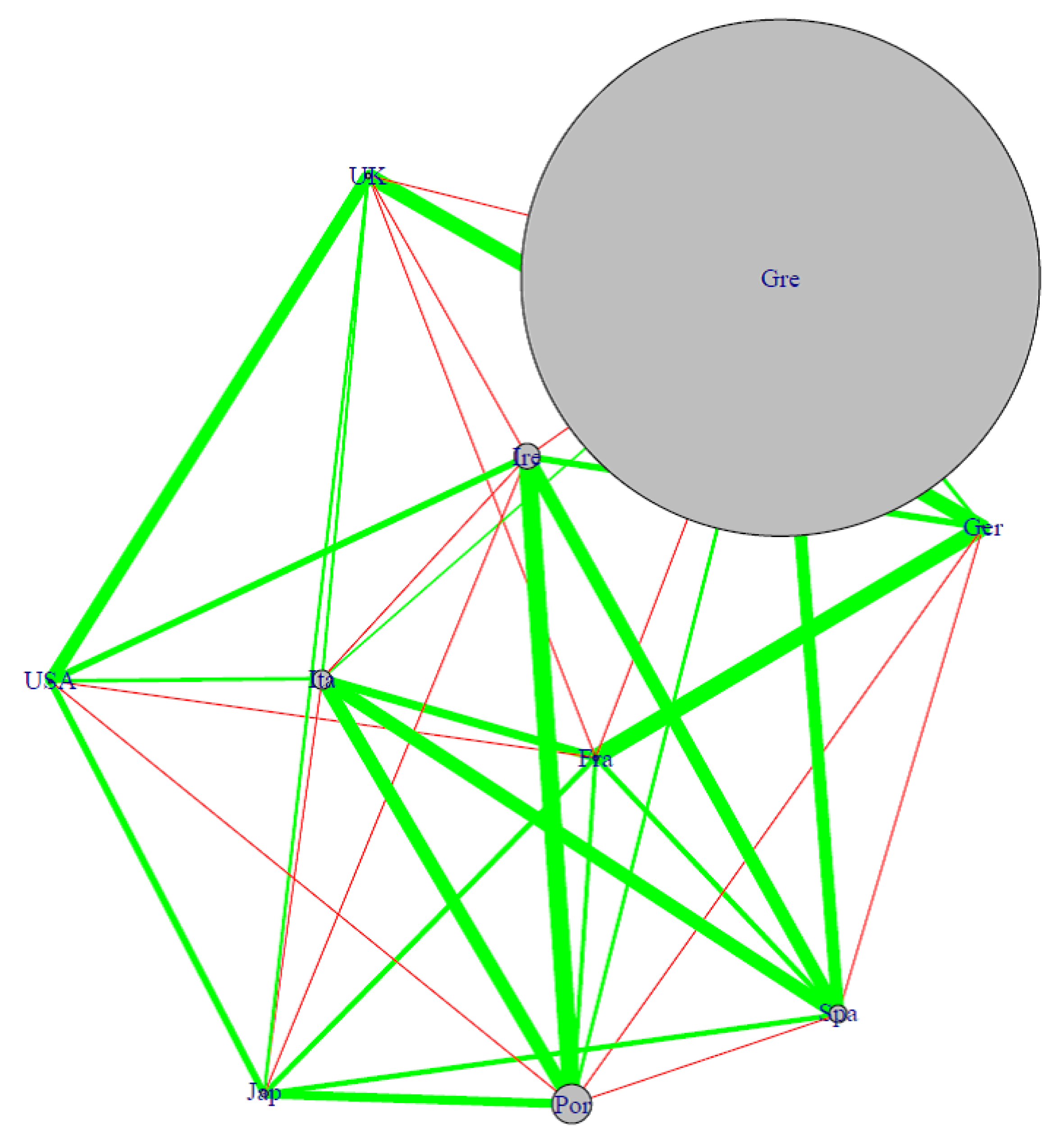
Figure 1 presents the partial correlation network between the considered countries, estimated using the entire time series. In the graph below, the larger a node, the larger its idiosyncratic default probability. Concerning edges between nodes, green lines stand for positive partial correlations, while red lines indicate negative partial correlations; the thicker the line, the stronger the connection. Absent connections correspond to conditional independencies.
Figure 1 clearly shows that the countries included in our sample are highly interconnected, with most partial correlations having a positive sign. The most central countries appear to be France and Italy: this is not a surprising result, and it is mainly due to the relevance of the European sovereign crisis within the considered time period, and to the fact that the sample mainly includes euro area countries. For a more precise understanding of the results shown in
Figure 1,
Table 2 presents the partial correlation values with the corresponding significance
t-tests. Each entry in
Table 2 can be considered as the weight (and the corresponding
t value) of the corresponding link in
Figure 1.
Table 2 indicates that the CDS spreads of some pairs of countries are indeed conditionally independent (their link is missing in
Figure 1). From an economic viewpoint, this means that they do not directly have an impact on each other. Such conditional independence affects the pairs (Greece, United States), (Greece, Japan), (Spain, United Kingdom), (Germany, United States).
Table 2 also reports countries with a negative direct correlation, for example: Germany with Spain and Portugal; Greece with France and Ireland; Ireland with Italy and Japan; the United States with France and Portugal. All these pairs of countries negatively impact each other, consistently with a “flight to quality” effect. Last, some countries appear to be strongly positively related, thus indicating a direct reciprocal contagion. This is the case of some pairs of core countries, such as (France, Germany), (Germany, UK), (UK, USA), but it also involves peripheral countries, like (Greece, Spain), (Ireland, Spain), (Spain, Portugal), (Italy, Spain), (Italy, Portugal).
The results described above indicate that contagion induces a “clustering effect”: core and peripheral countries further diverge through, and because of, contagion propagation, thus creating a sort of diabolic loop extremely difficult to be reversed. Core countries, with low CDS spreads, are unaffected by contagion, as they depend positively on each other and negatively with the peripherals. On the other hand, peripheral countries, with high CDS spreads, are impacted by contagion from other peripheral countries, and this effect is not mitigated by core countries as correlations with them are mostly negative.
We remark that, to our knowledge, the current study is the first one that allows for negative contagion. Negative contagion can be explained through capital flows: when a country i is facing a crisis period, investors tend to shift their portfolio towards “safer” places in order to reduce the level of risk (also called “fly-to-quality” behaviour): such places are typically the countries negatively related to i, thus implying an improvement in their survival probability. This mechanism justifies the difference between positive and negative risk propagation.
For robustness purposes, we also remark that we have calculated the partial correlation network separately for three time periods, more precisely: for the period ranging from 1 July 2006 to 31 December 2009 (financial crisis); for the period ranging from 1 January 2010 to 31 December 2012 (sovereign crisis); for the period ranging from 1 January 2013 to 31 December 2016 (post-crisis).
Figure 2 shows the corresponding results.
Figure 2 emphasises that the risk transmission mechanism has changed over the years: in the pre-crisis period, the overall number of significant partial correlations is quite high; during the financial crisis, the amount of strong partial correlation decreases; during the sovereign crisis, such amount further decreases and the “clustering effect” separating core and peripheral economies in two distinct subgroups emerges even stronger. Last, in the post-crisis period, the partial correlation pattern returns to the pre-crisis situation, however with a persisting clustering effect identifiable not only by positive within group (the two groups are the “core” and the “peripheral” countries) correlations, but also by negative correlations across the two groups. This overall mechanism finds the exception of Ireland, which seems to “migrate” from the periphery to the core relatively to the sample considered in this study.
4.3. VAR Model Estimation
As described in
Section 3, by means of partial correlations we can derive the
matrix and, then, the autoregressive parameters
. We are thus able to estimate the time-dependent CDS spreads of each country
i, and to disentangle the autoregressive idiosyncratic component from the contemporaneous
variable according to Equation (
2).
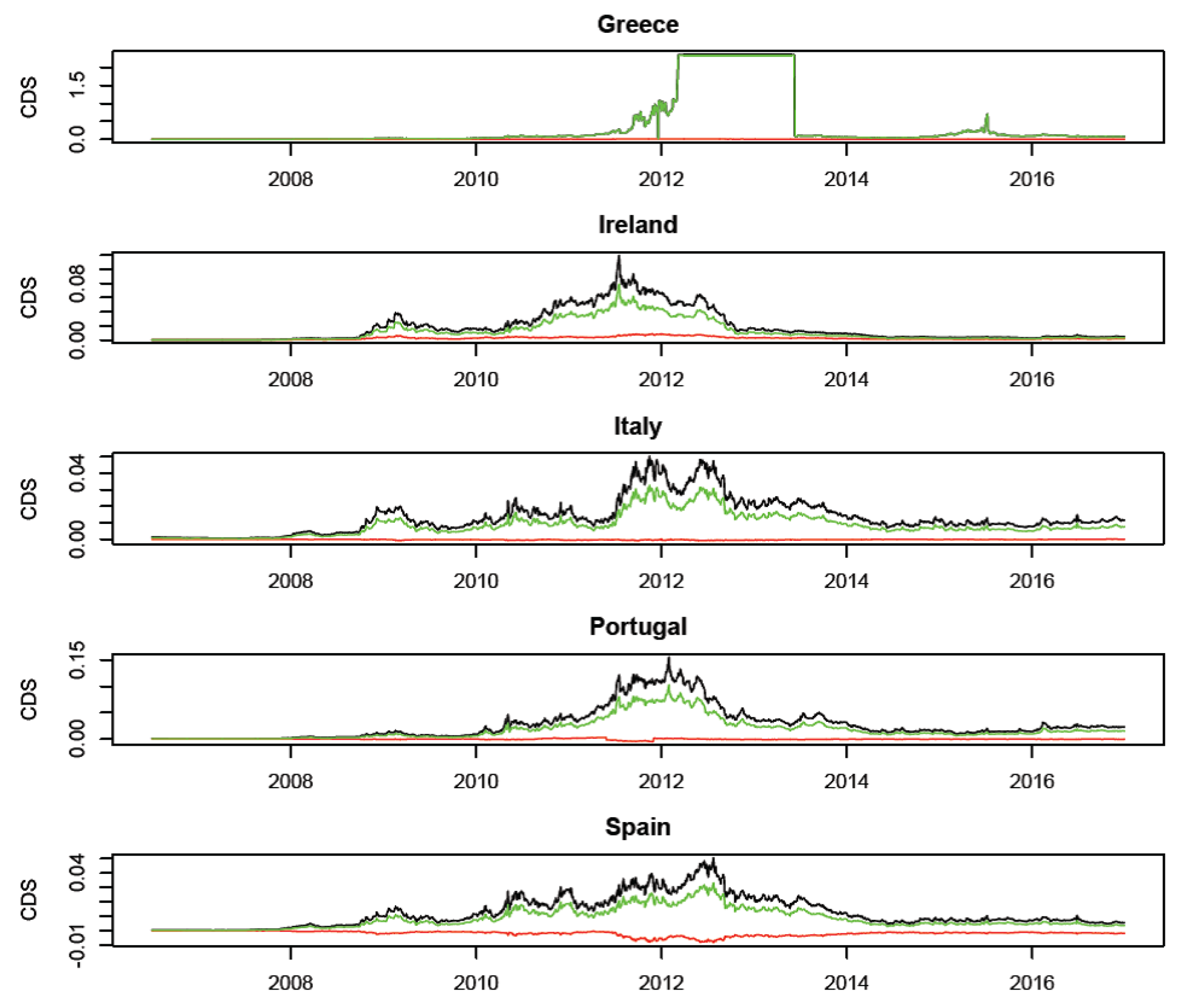
Figure 3 represents, for each of the five peripheral countries (namely Portugal, Ireland, Italy, Greece and Spain), the time evolution of the observed CDS spreads and of their estimated autoregressive and contemporaneous (
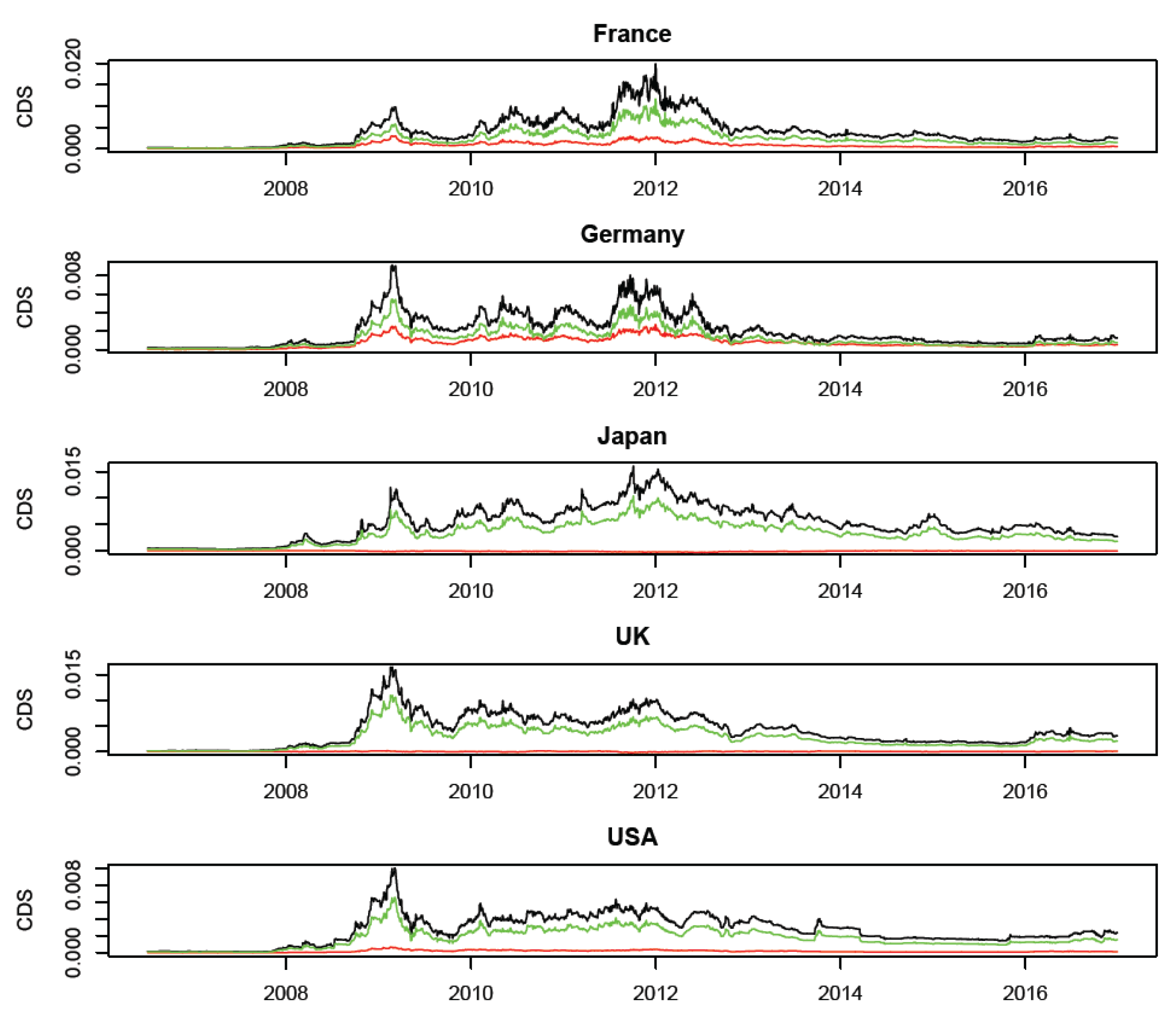
) components. The same graphs referred to core countries (France, Germany, Japan, the United Kingdom and the United States) are reported in
Figure 4.
Figure 3 shows that the autoregressive component prevails in peripheral countries, with a limited
effect in Ireland, Portugal and Spain.
Figure 4, instead, outlines that, although the autoregressive component prevails, there is a substantial contagion propagation affecting core countries: first and foremost France and Germany, which appeared to have strongly suffered the European sovereign crisis as risk importers. The Unites States and the UK have been more impacted in the previous time period, more precisely during the global financial crisis.
From an economic viewpoint,
Figure 3 and
Figure 4 can be jointly interpreted together with the network structure presented in
Figure 1: considering that peripheral economies are characterised by the highest idiosyncratic risk component, we can overall state that they are mainly “exporters” rather than “importers” of credit risk; on the contrary, core countries appear to be potential “importers” of credit risk.
4.4. CoRisk as a New Centrality Measure
In the financial network literature, a strong importance is assumed by the concept of “centrality measure” (of each node in the network, corresponding to single countries in our context). In qualitative terms, one node can be considered as “central” in a network if it is “highly interconnected” with the others, where the meaning of “highly interconnected” typically depends on the definition of “centrality” we assume a centrality measure thus aims at mapping such “centrality” feature by means of real numbers. As an example, the eigenvector centrality (see e.g.,
Furfine (
2003) and
Billio et al. (
2012)) considers as “more central” those nodes which are connected to other “highly central” nodes: based on this principle, the eigenvector centrality becomes a normalised score, assigned to each node, which takes the form of a real number
. This centrality measure can be easily calculated, for each country, from the correlation matrix between CDS spreads. Another measure of centrality is called degree of centrality, and it can also be easily obtained from the edge set
E by considering the number of significant links each country has with its neighbours.
Similarly, the
component of Equation (
2) gives, for each sovereign, a weighted (or normalised) degree of centrality, in which each binary link is replaced by the corresponding partial correlation coefficient. The resulting measure is intuitively expressed in basis points rather than in absolute numbers
.
Table 3 reports the comparison between the eigenvector centrality measure, calculated on the partial correlation matrix, and our
. It also reports the autoregressive component of Equation (
2).
Table 3 reveals that the most central countries in terms of eigenvector centrality are France, Germany, Italy and Spain: exactly the main players in the European sovereign crisis, either as importers (France, Germany) or exporters (Italy, Spain) of risk. Smaller European countries such as Portugal and Ireland follow. The United Kingdom and, more evidently, the United States and Japan, are less central in explaining the variations of CDS spreads in the considered period, consistently with the observed economic facts. Finally, Greece appears quite isolated, its crisis mainly due to idiosyncratic causes.
The
measure can shed further light on the interconnectedness between CDS spreads and on its interpretation. In particular, it can explain how much “net” contagion each country receives from/exports to the others, as measured by the increase/decrease of the CDS spread due to the contemporary component. In more detail, the
values reported in
Table 3 indicate that Greece is the country mostly impacted by contagion, followed by Ireland, France, Germany and, to a lesser extent, the United States and the United Kingdom: all these countries report a positive
value, indicating they are “importers” of risk (in line with the previous Section). On the contrary, Spain, Portugal, Italy and Japan report a negative
value, and they can thus be classified as “exporters” of risk.
From an economic viewpoint, the positive
of Greece indicates that this country is affected by the other countries to which it is most connected (see
Table 2), possibly because of funding problems. France and Germany, on the other hand, import risk from the peripheral countries to which they lend, through their credit risk channel. The positive
of Ireland indicates that the country has become an importer of risk, consistently with its recent economic recovery, which has shifted Ireland from the group of “peripherals” to the group of “core” economies. On a different note, the negative
of Italy, Portugal and Spain shows that these countries are “exporters” of contagion. This effect is stronger for Spain, whereas the other two peripheral countries, Portugal and Italy, show a limited impact as their exporting risk to core countries may be compensated by the import of risk from other peripherals (including Greece). Finally, the United States, Japan and the United Kingdom appear less central with respect to the sample of countries considered in this study: this is in line with the results obtained through the eigenvector centrality measure, and it shows that the U.S., Japan and the U.K. are relatively less linked to European peripheral sovereigns.
Overall, the empirical findings show that
can be interpreted as a centrality measure, and can indeed improve the interpretation of contagion by adding to the classical centrality measures introduced by
Furfine (
2003) a magnitude and a sign, which can both considerably improve economic interpretation. We remark that these outcomes have not needed the introduction of causal assumptions as done, for example, in Granger causality networks. We finally remark that the
and the autoregressive components, if summed together, determine an “average” estimate of CDS spreads that can be compared to the observed spreads reported in
Table 1: we can thus derive an overall measure of fit of the empirical model. It can be shown that the overall mean square error is equal to 274 bps against the 398 bps obtained with the model that contains only the autoregressive component: moreover, almost all the difference between the two errors is related to the contagion contributions of Greece, Portugal, Spain and Italy.
4.5. Robustness
For robustness purposes, in this section, we assess the predictive performance of our proposed model, especially to understand the impact of the contagion component with respect to a simple autoregressive formulation. More precisely, we run out of sample tests focused on the month in which the European sovereign crisis peaked: August 2011. We build our model using one year of daily data up to 31 July 2011. With the estimated model, we predict the CDS spreads for the whole month ahead, and compare the predictions with the observed spreads. We also compare our model with a simpler one, based on the autoregressive component only (so without the contemporaneous
effect).
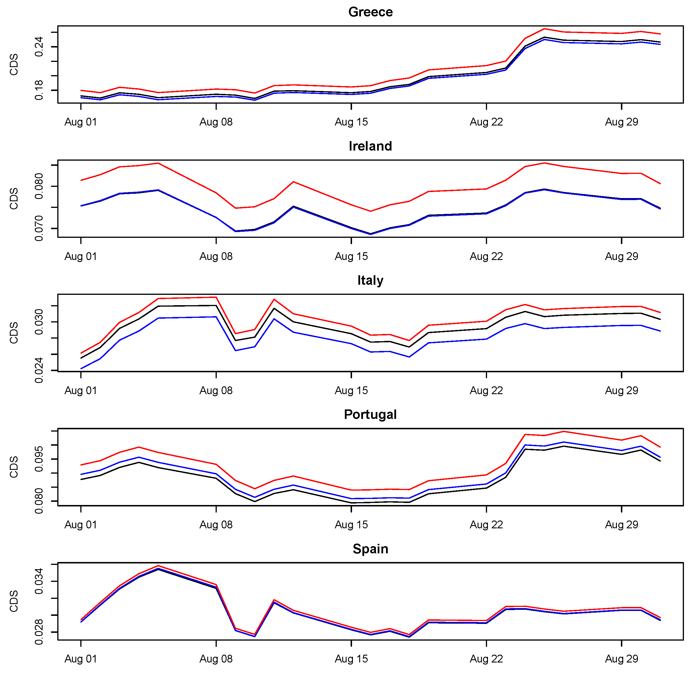
Figure 5 and
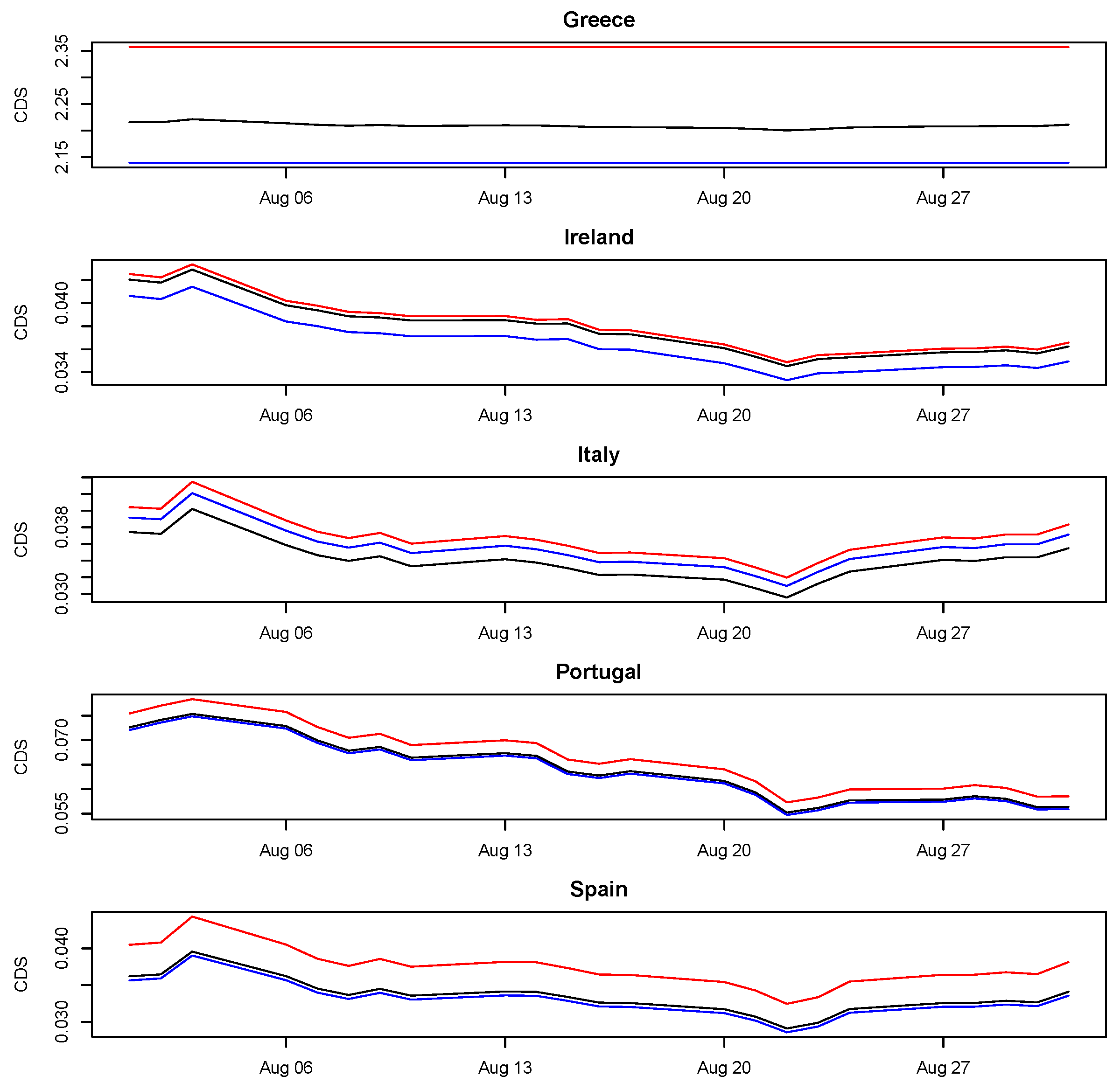
Figure 6 show, respectively for the five peripheral (Greece, Ireland, Italy, Portugal and Spain) and core (France, Germany, Japan, the United Kingdom and the United State) countries, a comparison between the observed and the predicted CDS spreads, using both the proposed model and the simpler model containing only the autoregressive component.
Both
Figure 5 and
Figure 6 reveal that the impact of the contagion component is not negligible, as shown by the comparison between our proposed model and the simpler autoregressive VAR: while the former always slightly overestimates CDS spreads, the latter strongly underestimates them. Such effect is slightly smaller for core countries with respect to peripheral ones, mainly because of their different magnitude scale of overall risk and, to a lesser extent, for their higher impact due to the contagion component. To provide a better explanation of the impact of the contagion component on our proposed model, and to fully compare our methodology with alternative proposals, we have identified the root mean square errors (RMSEs) as a summary metric. In particular,
Table 4 contains, for each country and for the entire sample, the RMSEs relative to a solely autoregressive component (RMSE only autoregressive) and to the full structural VAR as proposed in this study (RMSE full).
Consistent with the previous figures,
Table 4 shows that the impact of the
component increases the estimated CDS spreads with respect to the simple autoregressive component, thus increasing the predictive performance.
For robustness purposes, the same out-of-sample exercise performed above is now replicated focusing on a different time period, precisely on August 2012 (it is exactly the period that followed the ECB President Draghi’s “whatever it takes” famous speech). Similarly as before, we build the model using one year of daily data up to 31 July 2012. With the estimated parameters, we derive the CDS spreads for August 2012 and we compare them with the observed spreads. To understand the impact of the contagion component (
), we also include the results obtained by using a simple autoregressive model.
Figure 7 and
Figure 8 represent, respectively, for the five peripheral (Greece, Ireland, Italy, Portugal and Spain) and core (France, Germany, Japan, the United Kingdom and the United State) countries, a comparison between the observed and the predicted CDS spreads, using both the proposed model and the simpler model containing only the autoregressive component.
Figure 7 and
Figure 8 show that the situation is different with respect to the previous case on both core and peripheral counties, with all the risk components being much lower in August 2012 with respect to the same month of the previous year. In terms of relative impact of the
component on the overall predictive performance of the model, the two figures confirm the results obtained before. Finally,
Table 5 contains, for each country and for the entire sample, the RMSEs relative to a solely autoregressive component (RMSE only autoregressive) and to the full structural VAR as proposed in this study (RMSE full) referred to August 2012.
By comparing
Table 4 and
Table 5, it is clear that the predictive errors for August 2012 are on average higher than the errors obtained in the same month of the previous year: this is not surprising, since all countries (especially Greece) suffered from the sovereign crisis affecting Europe in 2012 and were thus experiencing a higher idiosyncratic risk. We finally remark that the predictive errors obtained in this section are lower than those commented on in the section discussing centrality measures: this can be explained recalling that, in these final robustness checks, models’ estimates and partial correlation matrices have been obtained by using only the previous year’s daily data instead of the whole time-sample. While recognising that the objective of the study is not forecasting CDS spreads, we are also aware that the caveats used in this last section can be considered as simplistic assumptions based on a static approach: this, however, does not affect the results in terms of impact of the contagion (
) component, which has been derived across different years (time-dimension) and countries (cross-sectional dimension).
5. Conclusions
In this work, we have proposed a new systemic risk measurement model, based on structural VAR processes for CDS spreads. Our main methodological contribution consists in the introduction of partial correlations and correlation networks into VAR models, in order to disentangle the autoregressive component (interpreted as idiosyncratic risk) and the contemporaneous part (interpreted as contemporaneous contagion effect) that we have named . In the context of CDS spreads, our proposed measure describes how many extra basis points should be paid to insure one monetary unit of a credit, when contagion is taken into account. Such contagion effect, moreover, can be both positive or negative: in the former case, it determines the spread to increase, typical behaviour of “risk-importer” countries; in the latter situation, it causes the spread to decrease, typical behaviour of “risk-exporter” countries.
By means of partial correlation networks, our results indicate that contagion induces a “clustering effect”: core and peripheral countries further diverge through, and because of, contagion propagation, thus creating a sort of diabolic loop extremely difficult to be reversed. Core countries, with low CDS spreads, are unaffected by contagion, as they depend positively on each other and negatively on the peripherals. On the other hand, peripheral countries, with high CDS spreads, are impacted by contagion from other peripheral countries, and this effect is not mitigated by core countries as correlations with them are mostly negative. From an interpretational viewpoint, when the is considered as a contagion centrality measure, it has a clear advantage over classic measures, being expressed in basis points rather than as absolute real numbers.
From an applied viewpoint, our empirical findings first show that the contagion effect, measured by , is strong within the euro area, especially in the largest economies (Germany, France, Italy, Spain). Second, this study confirms that peripheral countries mostly behave as exporters, rather than importers of system risk: as a consequence, core economies are (relatively) mostly affected by contagion risk, while peripheral countries strongly suffer from high idiosyncratic default probabilities with the notable exception of Greece (strongly suffering both). Finally, by means of out-of-sample tests, the contagion component of the model developed in this study is shown to have a significant impact on the overall predictive performance.
To summarise, the proposed variable appears to be not only a valid network centrality measure, but also an effective measure of contagion risk, which, while based on correlation networks, allows for drawing significant econometric findings that can help economic interpretation and predictive accuracy.
From an econometric viewpoint, the model could be generalised to the study of contagion among other country-specific financial indicators, or to the study of interconnectedness among other types of financial assets, with the limitation that the considered countries and/or assets should be kept constant over time.
From a policy-making viewpoint, the implications of our study are that contagion effects between the credit risk of different countries should be measured and taken into account and, therefore, mitigated. In the context of the Euro area, considered here, contagion can also strengthen the economical imbalances present between different countries, hampering financial stability.
We remark that our proposed methodology can be easily applied to other groups of countries, if the corresponding CDS spread time series are available. In particular, we believe that it would be interesting to apply our methods to the countries that are most affected by international financial contagion, either as large borrowers or as large lenders. Doing so, the effects of contagion could be measured and, thus, mitigated, for the sake of the global financial stability.


