General Quantile Time Series Regressions for Applications in Population Demographics

Abstract

The paper addresses three objectives: the first is a presentation and overview of some important developments in quantile times series approaches relevant to demographic applications—secondly, development of a general framework to represent quantile regression models in a unifying manner, which can further enhance practical extensions and assist in formation of connections between existing models for practitioners. In this regard, the core theme of the paper is to provide perspectives to a general audience of core components that go into construction of a quantile time series model. The third objective is to compare and discuss the application of the different quantile time series models on several sets of interesting demographic and mortality related time series data sets. This has relevance to life insurance analysis and the resulting exploration undertaken includes applications in mortality, fertility, births and morbidity data for several countries, with a more detailed analysis of regional data in England, Wales and Scotland.

1. Introduction

The theme of this tutorial is not to develop an analysis of all possible variants of quantile time series model: their model properties and relevant estimation approaches. Hence, the paper is not addressing the concerns of estimation of these models, as there is existing literature on these aspects in many cases. We provide references to relevant works on these aspects in several classes of models presented.

Instead, the focus is rather to provide a unified framework to construct such models for practitioners. Therefore, the emphasis of the paper is on the properties of the models and links between such models from a constructive perspective. As such, the tutorial takes a considered perspective on popular classes of quantile time series model structure that have been developed in the literature. It first introduces the key papers in the literature that have led to developments in some important classes of models. The second aspect of this paper is to provide an overview of various different model components that one can consider when developing a quantile times series models. This is the novelty introduced in this paper, where existing models are viewed from a different perspective and core components of relevance to general quantile time series modelling are decomposed and represented in components that allow development of new models and extensions of existing models.

In this regard, the theme of the overview is to decompose quantile time series modelling into a few core model components and then to go into detail on choices developed in the literature relating to these particular components. In viewing quantile time series modelling from this perspective, we are able to easily introduce new aspects to the modelling such as modifications to the quantile error function as well as nonlinear transformations of relevance to broader classes of quantile time series model.

In particular, in this paper, we consider classes of univariate quantile regression models developed in the context of time series modelling. We begin by providing a brief overview of different classes of parametric quantile time series regression models. Quantile valued time series models can be of many different types with regard to their regression structure: function on scalar or vector regressions; function on function regressions; and scalar on function regressions.

We then explore novel applications of quantile time series modelling in applications of relevance to life insurance contexts. In particular, we explore a range of mortality and demographic data sets via quantile time series regressions. The purpose of this is to illustrate for actuarial practitioners how one may utilise such time series modelling techniques to explore relevant demographic and mortality related time series data sets. The outputs of this analysis can be directly useful in insurance applications for instance in life insurance applications in annuities pricing and risk management as well as pension policy development. We do not go into detail on these particular areas of application; instead, we focus on modelling and comparison of different quantile time series models on these real mortality and demographic data sets obtained for England, Wales, Scotland and Northern Ireland.

In general, when studying such data sets, we note that one can separate such data sets typically into four categories1:

• Demographic data: which includes factors such as age, sex, migration patterns, ethnicity and marital status in populations. Typically, this comes from census type data sets.
• Health event data: this involves recordings of health events affecting individuals or populations which can include births, deaths, health conditions, primary care interactions, secondary care interactions and health hazards;
• Circumstantial data: focuses on aspects of individuals’ and populations’ circumstances that may affect the wider determinants of health, including socio-economic, lifestyle, and environmental data. Such data in this type of category can include education data; employment data; housing data and environmental data;
• National reference data: which includes data not collected for the sole purpose of health analysis; however, it can be used in connection with health data.

In this manuscript, we will focus on data reflecting demographic data and health event data. In Section 9, we provide a detailed overview of which data sets are considered. This will then be followed by the analysis of numerous quantile time series models, both linear and nonlinear, applied to these data sets. At each stage, a detailed description of the fitted model properties is provided in order to act as a guide for practitioners unfamiliar with such modelling approaches in demography and insurance.

Before we go into specific literature and background on quantile times series modelling, it would be remiss of us not to briefly mention some core developments of quantile regression contexts. The growth in general quantile regression modelling goes back to influential works by Koenker and Bassett 1978; Koenker 2005; Gilchrist 2000; Buchinsky 1998; Koenker 2004; Yu and Jones 1998 and in Bayesian modelling settings in Yu and Moyeed 2001; Thompson et al. 2010; Yu et al. 2003.

In addition, more recently, in Bernardi et al. (2016a), they extended the Bayesian family of Asymmetric Laplace distribution (ALD) quantile regression models to the family of Skewed Exponential Power (SEP) models. Their intention was to account for application settings in which the assumptions and model properties that standard ALD models impose was extended, allowing for greater skewness and kurtosis ranges to be feasibly expressed. In similar context, with the perspective of generalizing the distributional properties of the resulting quantile regression and its distributional tail properties, in Lancaster and Jae Jun (2010), they study applications of Bayesian exponentially tilted empirical likelihood to make inference about quantile regressions.

From the perspective of covariate selection and shrinkage in Bayesian quantile regressions, there is also a sequence of papers on regularization methods for quantile regressions, such as Li et al. (2010). In such works, the authors demonstrate that regularization methods such as lasso are effective in Bayesian quantile regression contexts. For a good overview of the past 40 years of quantile regression modelling over a wide spectrum of quantile models and modelling domains, see the discussions in Koenker (2017).

Quantile regression has also begun to be explored in more general regression settings such as for panel data applications, where bootstrap procedures are developed in such quantile regression contexts (see Galvao and Montes-Rojas (2015) and references therein).

The application of quantile regression models in financial risk and insurance has also recently begun to develop in works such as (Dong et al. 2015; Peters et al. 2016) and discussions in Operational risk contexts in (Cruz et al. 2015; Peters and Shevchenko 2015). Furthermore, there are Bayesian applications in econometrics. For instance, Hu et al. (2013) develop a Bayesian partially collapsed Gibbs sampler approach to fitting single-index models for conditional quantile regressions. In Bernardi et al. (2016b), they consider the challenge of model combining or model averaging in dynamic quantile regression settings, which they termed the general dynamic model averaging framework.

We now shift the focus from general quantile regression background to a particular focus on time series contexts. Specification of quantile function time series and regression can be decomposed into three main components:

• The conditional distribution of the regression time series model. This defines a conditional quantile function of the dependent variable, given the explanatory variables, primarily comprised in our case of time series past observations of the process. However, in general, the conditioning arguments may also include additional exogenous covariates perhaps with distributed lags;
• The structural component of the regression model. This component includes specification of the choice of link function and functional form expressing how covariates enter to the regression structure. The link function connected the linear or nonlinear predictor regression structure to the moments or parameters of the conditional quantile function;
• The actual choice of independent variables (regressors), that is, the covariates in the regression model and possible lagged and transformed structures. This could include distributed lags, projections, feature extraction as well as basis function transformations of the covariates.

1.1. Outline and Contributions

In Section 2, we overview important developments in the context of quantile regression modelling with a particular focus on quantile times series models.

In Section 3, Section 4 and Section 5, we present a general modelling framework for developing a wide class of quantile time series models that is detailed in a constructive manner involving four key ingredients. The first is the structural form of the quantile regression or time series model (linear or nonlinear maps), the second is the choice of quantile error function, the third is the choice of lag structure for the endogenous variables that characterize the quantile time series structure and the fourth is the choice of endogenous covariates and their lag structures. Then, we introduce examples in the case of non-parametric and parametric linear and nonlinear quantile time series models.

In Section 6, we characterize the class of quantile error function families in categories of location-scale, shape-scale and some special heavy tailed families of quantile functions. We conclude this section with discussion on truncated quantile error models for time series constructions with restricted supports.

In Section 7 and Section 8, we detail how to develop transformation of these basic families of parametric quantile error models to other significantly more flexible families of quantile error models based on two classes of mappings: the Tukey Elongation Maps and secondly the Rank Transmutation Map framework. We note that these general transformations may also be used to construct other aspects of the quantile time series model, not just the quantile error function.

In Section 9, we will explore applications of the general quantile time series model constructions on a range of demographic and mortality data. The focus will be to explore with applications the properties of some of the models discussed in the tutorial overview and to explore their application relevance for future developments in new insurance domains such as life-insurance modelling. We then conclude.

1.2. Notation

In this section, we briefly introduce some core notation used throughout the manuscript. We denote random variables by upper script and their realization by lower script. We denote vectors by bold and scalars by non-bold. Furthermore, we use the notation $Q_{Y_t}$ to refer to the quantile function of a random variable $Y_t$ obtained as the t-th time instance of a time series $\left\{Y_1,\dots ,Y_t,\dots \right\}$. We will typically refer to the quantile level by variable $u\in [0,1]$. The generic notation used for static model parameters in any of the introduced time series models will be denoted by vector $\mathit{\theta }$ unless otherwise discussed. Furthermore, we will utilize the notation ${\mathcal{F}}_t$ to denote the natural sigma-algebra of the observed time series given by ${\mathcal{F}}_t=\sigma (Y_1,\dots ,Y_t)$. We will therefore denote by $Q_{Y_t}\left(u|{\mathcal{F}}_{t-1};\mathit{\theta }\right)$ the conditional quantile function of random variable $Y_t$ condition on the information set ${\mathcal{F}}_{t-1}$, i.e., the observations of the time series until time $t-1$ given by $\left\{y_0,y_1,\dots ,y_{t-1}\right\}$ and the static model parameters generically denoted by $\mathit{\theta }\in {\mathbb{R}}^d$.

Furthermore, we will in general denote functional coefficients of the quantile time series structure by functions ${\alpha }_i(u)$ which will multiply lagged values of the time series. We will impose additional structure on these functions ${\alpha }_i(u)$ as required. When we consider the coefficients of lagged covariates, for a given quantile level u, we will also denote them by notations ${\mathit{\alpha }}_u=({\alpha }_{0,u},\cdots ,{\alpha }_{p,u})$ and ${\mathit{\beta }}_u=({\beta }_{0,u},\cdots ,{\beta }_{q,u})$ for u-th quantile coefficients. These could, for instance, be coefficients for the endogenous autoregressive (AR) structures and exogenous distributed lag structures, respectively, or for trend and volatility terms. In addition, we will denote by $Q_{ϵ}\left(u;\mathit{\gamma }\right)$ the quantile error function, which represents white noise sequence ${ϵ}_t$ with distributional static parameters generically denoted by $\mathit{\gamma }\in {\mathbb{R}}^{d^{\prime }}$. Additional notation used in the paper is introduced and defined where required.

2. Developments of Quantile Time Series Models

In its earliest form, quantile regression as introduced by Koenker and Bassett (1978) generalizes the notion of sample quantiles to linear and nonlinear regression models including the least absolute deviation estimation as its special case. In developing such a regression framework, one is able to develop estimation methods for conditional quantile functions at any (or all) probability levels. Such conditional quantile regression structures are now increasingly studied as they have been shown to present new information, compared to classical generalized linear model (GLM) regressions or linear mean regressions (see discussions in Koenker (2000)).

In (Koenker and Xiao 2006; Koenker 2017), the background of time series developments in quantile models is discussed for the class of quantile Autoregressive (QAR) models. Such QAR models are characterized by a parametric form, in the univariate time series $\left\{Y_t\right\}$ setting, by:

$$Q_{Y_t}\left(u|{\mathcal{F}}_{t-1};\mathit{\theta }\right)=\sum _{i=1}^p{\alpha }_i(u)Y_{t-i}+Q_{ϵ}\left(u;\mathit{\gamma }\right)$$

(1)

with notation as defined in Section 1.2.

To understand how to go from a time series model to a quantile time series model, consider the following relationship detailed in Example 1. This example illustrates the relationship between a functional, random coefficient AR time series model and its equivalent form expressed as a quantile time series model. Of course, any time series model, even without a structure of random functional coefficients can also admit a quantile time series model. However, in general the direct link between such a model and the coefficients of each model, the underlying time series model and the quantile time series model may not be easy to obtain in an explicit closed-form.

Example 1 (Relating Functional time series with Random Coefficients to Quantile time series).

Consider a functional time series model with random coefficients in an AR structure given by

$$\begin{array}{cc}\hfill y_t& =\sum _{i=1}^p{\alpha }_i(U_t)y_{t-i}+{\alpha }_0(U_t)\hfill \\ & =\sum _{i=1}^p{\alpha }_i(U_t)y_{t-i}+{ϵ}_t\hfill \end{array}$$

(2)

with $U_t\sim U[0,1]$ for all t and where ${\alpha }_i:[0,1]\mapsto \mathbb{R}$. We need only then assume that

$$\sum _{i=1}^p{\alpha }_i(U_t)y_{t-i}+{\alpha }_0(U_t)$$

is a monotone increasing function of $U_t$.

Note: one way to construct such a solution is to consider a positive valued time series, such that $Y_t\in {\mathbb{R}}^{+}$, then if each coefficient ${\alpha }_i(u):[0,1]\mapsto {\mathbb{R}}^{+}$ is specified as a quantile function which is scale invariant, one has that the resulting linear combination ${\sum }_{i=1}^p{\alpha }_i(U_t)y_{t-i}$ is a quantile function. Furthermore, one can write the equivalent conditional quantile function time series model as follows:

$$Q_{Y_t}\left(u|{\mathcal{F}}_{t-1};\mathit{\theta }\right)=\sum _{i=1}^p{\alpha }_i(u)y_{t-i}+{ϵ}_t,$$

(3)

which is obtained by use of the following general rule for any monotone increasing function g and standard uniform random variable U:

$$Q_{g(U)}\left(u\right)=g\left(Q_U(u)\right)=g(u),$$

(4)

where we use the fact that for a uniform random variable the distribution and quantile function satisfy the linear relationship, such that $F_U(u)=Q_U(u)=u$.

Such an example was illustrated in Koenker and Xiao (2006) where they point out that one can also consider, from a regression perspective, an alternative formulation of such functional regressions with scalar or vector on function regression. In particular, one can define a scalar (vector) on function regression version of the QAR model, with co-monotonic random functional coefficients, denoted as the random coefficients by

$$Y_t=\sum _{i=1}^p{\alpha }_i\left(U_t\right)Y_{t-i}+Q_{ϵ}\left(U_t;\mathit{\gamma }\right)$$

(5)

for i.i.d. $U_t\sim U(0,1)$. Such QAR models, in which the autoregressive coefficients are expressed as monotone functions of a single, scalar random variable are interesting as they allow one to capture

“systematic influences of conditioning variables on the location, scale and shape of the conditional distribution of the response, and therefore constitute a significant extension of classical constant coefficient linear time series models in which the effect of conditioning is confined to a location shift.”

(Koenker and Xiao 2006)

Furthermore, such quantile time series models can also be more robust to outliers and heavy tailed noise (see discussions in Fitzenberger et al. (2013)).

In the time series context, recent studies have also begun to develop properties specifically for QAR models, such as the notion of the quantile correlation (QACF) and quantile partial correlation (QPACF), defined in Li et al. (2015). These are natural quantile extensions of autocovariance and autocorrelation given by:

$${\mathrm{QACVF}}_u\left\{Y_t,Y_{t-\tau }\right\}=\mathbb{E}\left[\left(u-\mathbb{I}\left[Y_t-Q_{Y_t}(u)\right]\right)\left(Y_{t-\tau }-\mathbb{E}\left[Y_{t-\tau }\right]\right)\right],$$

(6)

$${\mathrm{QACF}}_u\left\{Y_t,Y_{t-\tau }\right\}=\frac{{\mathrm{QACVF}}_u\left\{Y_t,Y_{t-\tau }\right\}}{\sqrt{\mathbb{V}\mathrm{ar}\left(u-\mathbb{I}\left[Y_t-Q_{Y_t}(u)\right]\right)\mathbb{V}\mathrm{ar}\left(Y_{t-\tau }\right)}}.$$

(7)

In addition, an analogous QPACF can be obtained from the quantile based correlation and is given according to the expression in (Li et al. 2015, Equation (2.2)). Multivariate extensions have also been considered in Han et al. (2016) where they consider multiple QAR time series models, and develop the notion of cross-quantilogram. This provides a way to measure the quantile dependence between multiple quantile time series.

Variants of non-stationary QAR models have also been explored in Aue et al. (2017). This involves developing locally stationary QAR models through piece-wise, local in time constructions,

$$Q_{Y_t}\left(u|{\mathcal{F}}_{t-1};\mathit{\theta }\right)=\sum _{i=1}^{p_k}{\alpha }_{k,i}(u)Y_{t-i}+Q_{{ϵ}_k}\left(u;\mathit{\gamma }\right),$$

(8)

and they extend the standard QAR model to have a definition specific to each of the k segments. A detailed discussion of model selection and segmentation approaches is provided that performs local segmentation of the space and model selection per quantile level.

In the above discussion, we have not mentioned specific choices for the base quantile function $Q_{ϵ}\left(u;\mathit{\gamma }\right)$, this is a topic we will discuss in detail in later sections of this manuscript. However, we note that there are many ways to construct and decide upon such a reference quantile function. Recent developments in this context include the flexible class of non-parametric estimators proposed in Stephanou et al. (2017). In this work, they propose a simple non-parametric L-estimator class of kernel representations of the error quantile, based on the class of Hermite Askey-orthogonal polynomials. This builds on earlier works by (Cai 2002; Cai and Xu 2008) where non-parametric quantile time series modelling was studied via the inverse of weighted Nadaraya–Watson estimators of the conditional distribution function.

In addition to classes of QAR model, quantile time series regressions have been studied in both linear and nonlinear autoregressive settings in (Bloomfield and Steiger 1984; Cai 2010b; Cai et al. 2013; Weiss 1991; Davis and Dunsmuir 1997). The development of autoregressive conditional heteroscedasticity ARCH and GARCH models in quantile time series settings has also been undertaken by (Koenker and Zhao 1996; Lee and Noh 2013). Although the focus in this paper does not concern statistical estimation of quantile regression models, we believe it is still useful to mention that in frequentist estimation techniques for AR-ARCH type quantile models, identification in parameter estimation can be a challenge (see discussion in Noh and Lee (2015)). These authors demonstrate how a simple AR(1)-ARCH(1) model parametrized as follows:

$$\begin{array}{c}\hfill \begin{array}{cc}\hfill Y_t& ={\alpha }_0+{\alpha }_1{Y}_{t-1}+{ϵ}_t,\hfill \\ \hfill {ϵ}_t& ={\sigma }_t{\eta }_t,{\sigma }_t^2=\omega +\beta {ϵ}_{t-1}^2\mathrm{for}t\in \mathbb{Z},\hfill \end{array}\end{array}$$

(9)

with $\{{\eta }_t\}$ i.i.d. random variables satisfying $\mathbb{E}\left[{\eta }_t\right]=0$ and $\mathbb{E}\left[{\eta }_t^2\right]=1$, when re-expressed as a quantile regression form will have parameter identification issues. To see this, consider the reformulated AR(1)-ARCH(1) model represented as a quantile regression time series form as follows

$$\begin{array}{cc}\hfill Q_{Y_t}(u|{\mathcal{F}}_{t-1};\mathit{\theta })& ={\alpha }_0+{\alpha }_1{Y}_{t-1}+Q_{ϵ}\left(u;\mathit{\gamma }\right){\left(\omega +\beta {\left(Y_{t-1}-{\alpha }_0-{\alpha }_1{Y}_{t-2}\right)}^2\right)}^{1/2},\hfill \end{array}$$

(10)

where $Q_{ϵ}\left(u;\mathit{\gamma }\right)=inf\{x:P({ϵ}_1\le x;\mathit{\gamma })\ge u\}$. One may observe that since the u-th quantile of ${\eta }_t$ is unknown, then the parameters in Equation (10) are not identifiable. Fortunately, this issue can be overcome with appropriate re-parametrization of the model (see discussion in Lee and Noh (2013)).

The re-parametrized form, which is identifiable, is obtained by setting ${ϵ}_t=h_t{u}_t$, $h_t^2=1+\gamma {ϵ}_{t-1}^2$ with $h_t^2={\sigma }_t^2/\omega$, $u_t=\sqrt{\omega }{\eta }_t$ and $\gamma =\beta /\omega$. In such a re-parametrization, one has re-expressed the ARCH model as a conditional scale model with no scale constraints on the i.i.d. innovations. The resulting conditional quantile time series model is then given by

$$\begin{array}{cc}\hfill Q_{Y_t}(u|{\mathcal{F}}_{t-1};\mathit{\theta })& ={\alpha }_0+{\alpha }_1{Y}_{t-1}+Q_{ϵ}(u;\mathit{\gamma }){\left(1+\gamma {\left(Y_{t-1}-{\alpha }_0-{\alpha }_1{Y}_{t-2}\right)}^2\right)}^{1/2}.\hfill \end{array}$$

(11)

General results for parametrizations that extend beyond the AR-ARCH models to ARMA-AGARCH models which are identifiable are also developed in Noh and Lee (2015).

These developments were then presented in a general framework that is widely utilized, known as the Conditional Autoregressive VaR model (CAViaR) of Engle and Manganelli (2004). This model class has been extended to study explicitly models which have both conditional location and scale components (see Noh and Lee (2015)).

In Cai (2016) and then later in Noh and Lee (2015), the authors developed general classes of conditional location-scale quantile time series models based on time series models of the generic form:

$$\begin{array}{c}\hfill \begin{array}{c}\hfill Y_t={\mu }_t(\alpha )+{\sigma }_t(\alpha ){ϵ}_t\mathrm{for}t\in \mathbb{Z},\end{array}\end{array}$$

(12)

where ${\mu }_t(\alpha )$ and ${\sigma }_t(\alpha )$ were functions they used to denote $\mu (Y_{t-1},Y_{t-2},\dots ;\alpha )$ and $\sigma (Y_{t-1},Y_{t-2},\dots ;\alpha )$ for some measurable functions $\mu ,\sigma :{\mathbb{R}}^{\infty }\times {\mathrm{\Theta }}_1\to \mathbb{R}$; $\alpha$ denotes the true model parameter; ${\mathrm{\Theta }}_1$ is a model parameter space; $\{{ϵ}_t\}$ are i.i.d. random variables with an unknown common distribution function $F_{ϵ}$.

In fact, such ideas for quantile regression were previously well developed and explained in the location and scale class of quantile regression models in Gilchrist (2000). The equivalent quantile time series models may be presented according to the general location-scale generalized form given by

$$Q_{Y_t}\left(u|{\mathcal{F}}_{t-1},\mathit{\theta }\right)=\mu \left(Y_{t-1:t-p},\mathit{\alpha }\right)+\sigma \left(Y_{t-1:t-q},\mathit{\beta }\right)Q_{ϵ}\left(u;\mathit{\gamma }\right),$$

(13)

where model parameters $\mathit{\theta }=\left(\mathit{\alpha },\mathit{\beta },\mathit{\gamma }\right)$ with $\mathit{\alpha }=\left({\alpha }_0,{\alpha }_1,\dots ,{\alpha }_p\right)$, $\mathit{\beta }=\left({\beta }_0,{\beta }_1,\dots ,{\beta }_q\right)$ and generic quantile error function denoted by $Q_{ϵ}\left(u|\mathit{\gamma }\right)$.

Special cases of such models had previously also been considered in works such as Cai et al. (2013) who developed the quantile time series version of the double AR(p) models of Ling (2007) given by

$$Y_t={\alpha }_0+{\alpha }_1{Y}_t+\cdots +{\alpha }_p{Y}_{t-p}+{ϵ}_t\sqrt{{\beta }_0+{\beta }_1{Y}_{t-1}^2+\cdots +{\beta }_q{Y}_{t-q}^2},$$

(14)

where ${\beta }_i>0$ for $i\in \left\{0,\dots ,q\right\}$, ${ϵ}_t\stackrel{i.i.d.}{\sim }N(0,1)$ and $Y_t$ is independent of ${ϵ}_t$ for all t.

As noted in Cai et al. (2013), this is a special case of the ARMA-ARCH models proposed by Weiss (1984); however, it is structurally distinct from the ARCH models proposed by Engle (1982) when one considers settings in which ${\alpha }_i\ne 0$. A further extension developed includes the Double-QAR(p,q) model of Cai et al. (2013) given by

$$Q_{Y_t}\left(u|{\mathcal{F}}_{t-1},\mathit{\theta }\right)={\alpha }_0+{\alpha }_1{Y}_t+\cdots +{\alpha }_p{Y}_{t-p}+\sqrt{{\beta }_0+{\beta }_1{Y}_{t-1}^2+\cdots +{\beta }_q{Y}_{t-q}^2}{Q}_{ϵ}\left(u;\mathit{\gamma }\right),$$

(15)

where model parameters $\mathit{\theta }=\left(\mathit{\alpha },\mathit{\beta },\mathit{\gamma }\right)$ with $\mathit{\alpha }=\left({\alpha }_0,{\alpha }_1,\dots ,{\alpha }_p\right)$ and $\mathit{\beta }=\left({\beta }_0,{\beta }_1,\dots ,{\beta }_q\right)$. In this particular study, the quantile error distribution was selected as a flexible quantile sub-family of the generalized lambda family of distributions developed in Freimer et al. (1988).

Other forms of nonlinear quantile time series models have been explored, such as the class of quantile self-exciting threshold autoregressive time series models proposed in Cai and Stander (2008). Such models are the quantile time series extension of self-exciting threshold autoregressive time series (SETAR) models, often referred to as the class of QSETAR models. These are generally characterized by the QAR model extension given by:

$$Q_{Y_t}\left(u|{\mathcal{F}}_t\right)=\sum _{i=1}^{m+1}\left[\left(\sum _{j=1}^p{\alpha }_{i,j}(u)Y_{t-j}\right)+Q_{{ϵ}_{i,t}}(u)\right]\mathbb{I}\left\{y_{t-d}\in (y_{i-1},y_i]\right\},$$

(16)

where we consider the following state-space threshold partitions $-\infty =y_0<y_1<\cdots <y_{m+1}=\infty$ and denote by $\mathbb{I}\left\{·\right\}$ the indicator function taking value one, when the arguments condition is satisfied and zero otherwise.

Other classes of nonlinear quantile time series models developed include those studied in (Peters et al. 2016; Dong et al. 2015; Chen et al. 2017) where they proposed nonlinear quantile models of the form

$$Q_{Y_t}(u|{\mathcal{F}}_{t-1},\mathit{X};\mathit{\theta })=T\left({\mathcal{F}}_t,{\mathcal{G}}_t,Q_{ϵ}(u;\mathit{\gamma })\right),$$

(17)

which characterize the class of quantile models equivalent to distributed lag ARDL models with exogenous covariates. Furthermore, these models were also extended in Chen et al. (2017) to quantile state-space models (QSSM) that they termed the AQUA class. In Peters et al. (2016), several classes of transform function $T(·)$ were explored based on the Tukey class of elongation transforms, including popular sub-classes of g-and-h, G-and-K, G-and-J, G-G, and H-H transforms. An efficient R-package for estimation and description of its functionality is provided by Prangle (2017).

In terms of forecasting of quantile time series models, there are multiple approaches one can adopt (see discussions in Cai (2010a)). Furthermore, there is a branch of quantile time series models relating to extreme value theory (see a detailed discussion in McNeil and Frey (2000)). To complete this section, we make the following example to illustrate a general mapping from a time series model to a quantile time series model.

Example 2 (Relating General Nonlinear Stochastic Volatility Time Series Models to Quantile Time Series Models).

Consider a functional time series model characterized by the general structural form

$$\begin{array}{cc}\hfill Y_t& =\mu \left(Y_{t-p},\dots ,Y_{t-1};\mathit{\theta }\right)+\sum _{j=1}^q{\theta }_j\sigma \left(Y_{t-s-q},\dots ,Y_{t-1-q},t;\mathit{\gamma }\right){\alpha }_0(U_{t-q})+\sigma \left(Y_{t-s},\dots ,Y_{t-1},t\right){\alpha }_0(U_t)\hfill \\ & =\mu \left(Y_{t-p},\dots ,Y_{t-1}\right)+\sum _{j=1}^q{\theta }_j\sigma \left(Y_{t-s-q},\dots ,Y_{t-1-q},t\right){ϵ}_{t-q}+\sigma \left(Y_{t-s},\dots ,Y_{t-1},t\right){ϵ}_t\hfill \end{array}$$

(18)

for time t and where $U_t$ is an i.i.d. sequence of uniform random variables $U_t\sim U[0,1]$ and where ${\alpha }_0:[0,1]\mapsto \mathbb{R},$ which we assume satisfies that ${\alpha }_0(u)$ is a monotone increasing function in $U_t$.

Furthermore, we assume a general parametric linear or nonlinear map $\mu \left(Y_{t-p},\dots ,Y_{t-1},t;\mathit{\theta }\right)$ of lagged values of the process $Y_t$ and time t for the trend such that $\mu :{\mathbb{R}}^p\times {\mathbb{R}}^{+}\mapsto \mathbb{R}$ parametrized by model parameters generically denoted by $\mathit{\theta }$ and a nonlinear stochastic volatility structure given by functional form $\sigma \left(Y_{t-s},\dots ,Y_{t-1};\mathit{\gamma }\right)$ such that $\sigma :{\mathbb{R}}^s\mapsto {\mathbb{R}}^{+}$ with generic model parameters $\mathit{\gamma }$. Then, in this case, one has the general equivalent conditional quantile function time series model can be obtained, under the restrictions that ${\theta }_i\ge 0$ for $i\in \left\{1,\dots ,q\right\}$, given by

$$\begin{array}{cc}\hfill Q_{Y_t}\left(u|{\mathcal{F}}_{t-1};\mathit{\theta }\right)& =\mu \left(Y_{t-p},\dots ,Y_{t-1}\right)+\sum _{j=1}^q{\theta }_j\sigma \left(Y_{t-s-q},\dots ,Y_{t-1-q},t\right)Q_{{ϵ}_{t-q}}(u)+\sigma \left(Y_{t-s},\dots ,Y_{t-1},t\right)Q_{{ϵ}_t}(u)\hfill \\ & =\mu \left(Y_{t-p},\dots ,Y_{t-1}\right)+Q_{\widetilde{{ϵ}_t}}\left(u|{\mathcal{F}}_{t-1};{\mathit{\theta }}_{1:q},\right).\hfill \end{array}$$

(19)

To obtain this representation, we use the fact that a positive scaling of a quantile function is a quantile function, such that for all $t,s,q$ on has that ${\theta }_j\sigma \left(Y_{t-s-q},\dots ,Y_{t-1-q},t\right)Q_{{ϵ}_{t-q}}(u)$ is a quantile function. Furthermore, any linear combination of quantile functions is also a quantile function and we apply the rule that a linear translation of a quantile is a quantile function. Finally, we are back to the condition that we may then apply again the following general rule for any monotone increasing function g and standard uniform random variable U:

$$Q_{g(U)}\left(u\right)=g\left(Q_U(u)\right)=g(u),$$

(20)

where we use the fact that for a uniform random variable the distribution and quantile function satisfy the linear relationship such that $F_U(u)=Q_U(u)=u$.

Remark 1.

The above example is intended to be illustrative of the general approach one can adopt to moving from time series models to the equivalent relationship in a quantile time series model. However, one must in general still be cautious to consider such general model structures from the perspective of estimation and appropriate identification considerations.

3. General Construction of Quantile Time Series Regression Models

In the literature, it is common to develop quantile time series models dependent only on endogenous variables in the regression structure. In other words, the vast majority of time series quantile regression models discussed are constructed from conditional distributions which are based on information filtration, denoted ${\mathcal{F}}_t=\sigma \left(Y_0,\dots ,Y_t\right),$ which is constructed from the sigma-algebra naturally generated by the time series signal under consideration.

However, in many practical settings, it will be of interest to extend the class of quantile time series models such as the QAR models to include lagged endogenous covariates of different forms. A first natural extension would be to begin by developing the conditional quantile function forming the time series to also be dependent explicitly on a second filtration of observed exogenous covariates, which will be denoted by ${\mathcal{G}}_t=\sigma \left({\mathit{X}}_0,\dots ,{\mathit{X}}_t\right)$, where ${\mathit{X}}_t\in {\mathbb{R}}^d$.

In such cases, one can construct a range of extensions of the QAR model, for instance, such as the two illustrative examples below:

$$\begin{array}{cc}\hfill Q_{Y_t}\left(u|{\mathcal{F}}_{t-1},{\mathcal{G}}_t;\mathit{\theta }\right)& =\sum _{i=1}^p{\alpha }_i(u)Y_{t-i}+\sum _{j=1}^d\sum _{i=1}^k{\beta }_{j,i}{X}_{j,t-i}+Q_{ϵ}\left(u;\mathit{\gamma }\right),\hfill \\ \hfill Q_{Y_t}\left(u|{\mathcal{F}}_{t-1},{\mathcal{G}}_t;\mathit{\theta }\right)& =\sum _{i=1}^p{\alpha }_i(u)Y_{t-i}+\sum _{j=1}^d\sum _{i=1}^k{\beta }_{j,i}{Q}_{X_{j,t-i}|X_{j,1:t-i}}(u)+Q_{ϵ}\left(u;\mathit{\gamma }\right),\hfill \end{array}$$

(21)

where in the second case one may wish to impose that ${\beta }_{j,i}>0$ for all $i,j$ to ensure the resulting conditional quantile function is well defined. These illustrative models are based on linear relationships in the quantile time series regressions. However, we will also consider the general class of nonlinear and linear cases generically presented by the following parametric conditional quantile relationship

$$Q_{Y_t}\left(u|{\mathcal{F}}_{t-1},{\mathcal{G}}_t;\mathit{\theta }\right)=T\left({\mathcal{F}}_t,{\mathcal{G}}_t,Q_{ϵ}(u)\right),$$

(22)

which involves some form of quantile preserving map defined in detail in the following sections. We will overview several classes of such mappings from the literature, including classical approaches based on location-scale, shape-scale maps as well as more advanced approaches such as the Rank Transmutation Maps (RTM) and the Elongation transforms of Tukey.

Remark 2 (Characterizing Generalized Quantile time series Models).

To characterize this general class of quantile time series models, we will consider defining six attributes:

1. 

choice of mapping function $T(·)$ which can be linear or nonlinear on the quantile error function or on the quantile function time series “trend” structure;

2. 

the choice of quantile error function $Q_{ϵ}(u)$—if in the parametric model context;

3. 

the inclusion or not of lagged observations of the time series of interest ${\left(Y_t\right)}_{t\ge 0}$, obtained by the natural filtration generated by the realization of the process (denoted ${\mathcal{F}}_t$), which enter in the model in either the location or the scale or both;

4. 

the inclusion or not of lagged exogenous covariates generically denoted by set of vectors ${\mathit{x}}_t=\left(x_{1,t},\dots ,x_{d,t}\right)$, obtained by the natural filtration generated by the realization of the process (denoted ${\mathcal{G}}_t$), which enter in the model in either the location or the scale or both;

5. 

the choice of parametric vs. non-parametric model, through either an explicit specification of a quantile error function $Q_{ϵ}(u)$ for the model, or a non-parametric approach when no quantile function is explicitly considered;

6. 

function on function regressions, when one models the entire quantile function by considering all quantile levels $u\in [0,1]$ or some sub-set of this range, versus individual quantile regressions for a specific target quantile level u.

In the following sub-sections, we discuss each of these components in turn, starting with the distributional aspects of the quantile regression models we consider. In this regard, the models of particular focus in this tutorial are the following classes of quantile model:

• the Asymmetric Laplace (AL) distribution;
• the regularly varying and heavy tailed classes of power-law distributions, which may for instance be characterized by models whose hazard rate $r(y)$ given by

  $$r(y)=\frac{f_Y(y)}{{\overline{F}}_Y(y)},$$

  (23)

  satisfies the condition for instance in the right tail that

  $$\underset{y\to \infty }{lim}r(y)=0;$$

  (24)
• one, two, three and four parameter parametric distributional models often occurring as sub-members of the Pearson family and the Exponential family and is dispersion extensions.
• the Rank Transmutation composite quantile function maps
• the Tukey g-and-h elongation transform family,

which we extend to classes of quantile time series models.

We begin with an overview of some core examples of non-parametric quantile time series models and how these relate to the Asymmetric Laplace parametric model. We then proceed with more detailed illustrations of parametric modelling of quantile time series.

4. Nonparametric Quantile Time Series Models

In this case, we will consider the sub-class of regression quantile time series models given by

$$Q_{Y_t}(u)=T\left({\mathcal{F}}_t,{\mathcal{G}}_t\right),$$

(25)

where we drop from the transformation $T(·)$ the component corresponding to the quantile error distribution specification $Q_{ϵ}(u)$, hence making the model non-parametric in nature.

4.1. Examples of Linear Nonparametric Quantile Time Series Models

In a non-parametric quantile regression time series approach, one seeks to estimate regression coefficients without the need to make any assumptions on the distribution of the response, or equivalently the residuals. To understand this, we will first introduce a simple quantile AR process. We will focus on the family of models to begin with that have a linear transformation i.e., where the mapping $T(·)$ is considered to be a simple linear function of the coefficients. Furthermore, we will consider a specific target quantile level u in the initial set-up below, not a functional regression structure.

Definition 1  (Non-Parametric Quantile Autoregressive QAR(p) Time Series).

Consider the time series ${(Y_t)}_{t\ge 0}$; then, the quantile time series model is defined according to the conditional quantile functions as follows:

$$Q_{Y_t}(u|{\mathcal{F}}_t)={\alpha }_{0,u}+\sum _{k=1}^p{\alpha }_{k,u}{y}_{t-k}.$$

(26)

One may consider ${\mathcal{F}}_t$ to be the natural filtration generated by the observed time series ${\left(Y_t\right)}_{t\ge 0}$ up to the current time point, or it may contain additional structure such as lagged covariates. The location of the u-th quantile level is determined by coefficient scaled lagged previous values of the time series, where the coefficients can be quantile level specific. The coefficients are characterized as the solution to the system of equations, for all $s\in \left\{1,\dots ,t,\dots \right\}$ given by:

$$\mathbb{P}\mathrm{r}\left[y_s\le {\alpha }_{0,u}+\sum _{k=1}^p{\alpha }_{k,u}{y}_{s-k}|{\mathcal{F}}_s\right]=u,$$

(27)

when such a solution exists.

Remark 3.

Note, in this non-parametric specification, no distributional assumption is being made regarding the conditional distribution for $Y_t|{\mathcal{F}}_t$, so, at this stage, one may wonder how can the coefficients ${\mathit{\alpha }}_u$ be estimated. The answer involves reformulating the coefficients as the solution of a loss function minimization, which does not require any distributional assumptions to be made on the time series marginal or conditional distributions.

This reformulation is given by the quantile loss function. Hence, we may analogously obtain estimates of the quantile model parameters, non-parametrically by solving the following loss function minimization:

$$\underset{{\alpha }_{0,u},\cdots ,{\alpha }_{p,u}}{min}\sum _t{\rho }_u({ϵ}_t)=\sum _t{ϵ}_t[u-I({ϵ}_t<0)]$$

(28)

and ${ϵ}_t=y_t-{\alpha }_{0,u}-{\displaystyle \sum _{k=1}^p}{\alpha }_{k,u}{y}_{t-k}$.

Furthermore, it has been shown in (Koenker and Hallock 2001; Koenker and Machado 1999; Yu and Moyeed 2001) that under this loss function ${\rho }_u$ for quantile regression, the parameter estimates of ${\mathit{\alpha }}_u$, which may be obtained by minimizing the loss function in (28) will be equivalent to the maximum likelihood estimates of ${\mathit{\alpha }}_u$ when the conditional distribution of $Y_t|{\mathcal{F}}_t$ follows the Asymmetric Laplace proxy distribution given in Definition 2.

Definition 2 (Asymmetric Laplace Distribution).

A random variable $X\sim AL(\mu ,\sigma ,p)$ has an Asymmetric Laplace (AL) law if it has the following distribution and density

$$\begin{array}{cc}\hfill F(x;\mu ,\sigma ,p)& =\left\{\begin{array}{cc}\frac{\sigma }{p+1/p}exp\left[\frac{\sigma }{p}(x-\mu )\right]\hfill & \mathit{if}x<\mu ,\hfill \\ \frac{\sigma }{p+1/p}exp\left[-\sigma p(x-\mu )\right]\hfill & \mathit{if}x\ge \mu ,\hfill \end{array}\right.\hfill \\ \hfill f(x;\mu ,\sigma ,p)& =\left(\frac{\sigma }{p+1/p}\right)exp\left[-(x-\mu )\sigma s{p}^s\right],\hfill \end{array}$$

(29)

where $s=sgn(x-\mu )$, $\mu \in \mathbb{R}$ is the location; $\sigma >0$ is the scale parameter; and p is the asymmetry parameter. The mean, variance, skewness and kurtosis of this model are given by:

$$\begin{array}{ccc}\hfill \mathbb{E}\left[X\right]& =& \mu +\frac{\sigma (1-2p)}{p(1-p)},\mathbb{V}\mathit{ar}[X]=\frac{{\sigma }^2(1-2p+2p^2)}{{(1-p)}^2{p}^2},\hfill \end{array}$$

(30)

$$\begin{array}{ccc}\hfill S[X]& =& \frac{2[{(1-p)}^3-p^3]}{{({(1-p)}^2+p^2)}^{3/2}},K[X]=\frac{9p^4+6p^2{(1-p)}^2+9{(1-p)}^4}{{(1-2p+2p^2)}^2}.\hfill \end{array}$$

(31)

Note, when $p=1$, we have that the AL distribution simplifies to the well known Laplace distribution. Hence, we may now observe that this family of distributions contains, embedded in the exponential argument, exactly the component required for minimization in the quantile regression loss function. This allows us to write the problem of solving for the coefficients of the model in Definition 1 given by:

$$f(y_t|{\mathcal{F}}_t;{\mu }_t,{\sigma }^2,p)=\frac{p(1-p)}{\sigma }exp\left(-\frac{(y_t-{\mu }_t)}{\sigma }[p-I(y_t\le {\mu }_t)]\right)$$

(32)

for the location parameter or mode ${\mu }_t$, the scale parameter $\sigma >0$ and the skewness parameter $p\in (0,1)$ equals to the quantile level u. Since the pdf (32) contains the loss function (28), it is clear that parameter estimates that maximize Equation (32) will minimize Equation (28).

In this formulation, the AL distribution represents the conditional distribution of the observed dependent variables (responses) given the covariates. More precisely, the location parameter ${\mu }_t$ of the AL distribution links the coefficient vector ${\mathit{\alpha }}_u$ and associated covariates in the linear time series regression model to the location of the AL distribution.

4.2. Examples of Nonlinear Nonparametric Quantile Time Series Models

A natural extension of the QAR(p) class of quantile time series models is to consider the nonlinear class of non-parametric models. Here, we are treating the mapping $T(·)$ as comprised of a combination of nonlinear and potentially also linear components.

Under the representation presented for the QAR(p) model, and its embedding within the AL family for estimation convenience, it is straightforward to extend the quantile regression model to allow for heteroscedasticity in the response, which may vary as a function of the quantile level u under study. To achieve this, one can simply add a regression structure linked to the scale parameter ${\sigma }_t$ in the same manner as was done for the location parameter.

This would correspond to what we will call the Dynamic Volatility QAR(p) time series model given in the following definition.

Definition 3 (Examples of Non-Parametric Dynamic Volatility Quantile Autoregressive DV-QAR(p,q) Time Series).

Consider the time series ${(Y_t)}_{t\ge 0}$; then, the DV-QAR(p) quantile time series model is defined according to the conditional quantile functions as follows:

$$Q_{Y_t}(u|{\mathcal{F}}_t)={\alpha }_{0,u}+\sum _{k=1}^p{\alpha }_{k,u}{y}_{t-k}$$

(33)

with

$$\mathbb{V}\mathit{ar}\left[Y_t|{\mathcal{F}}_t\right]=\frac{1+u^4}{{\sigma }_t^2{u}^2}=\frac{1+u^4}{u^2}{\left({\beta }_{0,u}+\sum _{k=1}^q{\beta }_{k,u}{y}_{t-k}\right)}^{-2},$$

(34)

where ${\mathcal{F}}_t$ denotes information set or filtration that defines the time series dynamic. For instance, ${\mathcal{F}}_t$ may be the natural filtration generated by the observed time series ${\left(Y_t\right)}_{t\ge 0}$ up to the current time point, or it may contain additional structure such as lagged covariates. The notation, $u\in (0,1)$, corresponds to the quantile level, and location of the u-th quantile level is dictated by coefficient lagged previous values of the time series, where the coefficients can be quantile level specific. The coefficients are characterized as the solution to the system of equations, for all $s\in \left\{1,\dots ,t,\dots \right\}$ given by:

$$\mathbb{P}r\left[y_s\le {\alpha }_{0,u}+\sum _{k=1}^p{\alpha }_{k,u}{y}_{s-k}|{\mathcal{F}}_s\right]=u,$$

(35)

subject to the constraint for the filtration ${\mathcal{F}}_t$ given by

$$\begin{array}{c}\frac{1}{t-1}\sum _{s=1}^t{\left\{y_s-\left[{\alpha }_{0,u}+\sum _{k=1}^p{\alpha }_{k,u}{y}_{s-k}+\frac{1-u^2}{u}\left({\beta }_{0,u}+\sum _{k=1}^q{\beta }_{k,u}{y}_{t-k}\right)\right]\right\}}^2\hfill \\ =\frac{1+u^4}{u^2}{\left({\beta }_{0,u}+\sum _{k=1}^q{\beta }_{k,u}{y}_{t-k}\right)}^{-2}\hfill \end{array}$$

(36)

when such a solution exists.

Remark 4.

This second constraint in the above definition of the DV-QAR(p) process imposes the restriction that the time series process will admit a representation in which the original time series ${\left(Y_t\right)}_{t\ge 0}$ will be heteroskedastic with a volatility given by the functional specification:

$$\mathbb{V}\mathit{ar}\left[Y_t|{\mathcal{F}}_t\right]=\frac{1+u^4}{{\sigma }_t^2{u}^2}=\frac{1+u^4}{u^2}{\left({\beta }_{0,u}+\sum _{k=1}^q{\beta }_{k,u}{y}_{t-k}\right)}^{-2}.$$

(37)

In terms of fitting such a DV-QAR(p) model, it will be convenient to observe the following relationship between this non-parametric model and its embedding withing a parametric AL distributional model.

Remark 5 (Embedding of the non-parametric DV-QAR(p) within Scale-Location Varying Asymmetric Laplace Model).

Equivalently, we assume that $Y_t|{\mathcal{F}}_t$ conditionally follows an AL distribution denoted by $Y_t|{\mathcal{F}}_t\sim AL({\mu }_t,{\sigma }_t^2,u)$. Then,

$$Y_t={\mu }_t+{ϵ}_t{\sigma }_t,$$

(38)

where ${ϵ}_t\sim AL(0,1,u)$, the location and scale dynamic functions are given by

$$\begin{array}{cc}\hfill {\mu }_t& ={\alpha }_{0,u}+\sum _{k=1}^p{\alpha }_{k,u}{y}_{t-k},\hfill \\ \hfill {\sigma }_t^2& =exp({\beta }_{0,u}+\sum _{k=1}^q{\beta }_{k,u}{y}_{t-k}).\hfill \end{array}$$

(39)

Discussion on the parametric regression model, in particular, the choice of link function and structure of regression terms will be undertaken in later sections.

Note: this representation has the following advantages:

• the parameters can be estimated by maximum-likelihood under the AL distribution family; and
• importantly, it links the quantile process to a linear (when ${\sigma }_t=\sigma$) AR process with a driving noise sequence given by an AL error with appropriately chosen asymmetry parameter for $p=u$ corresponding to the target quantile level.

Other examples of nonlinear time series models have been proposed in the literature such as the double-AR time series structures of Cai et al. (2013), which we modify below to the non-parametric specification, embedded within an AL distribution estimation framework as noted in the DV-QAR(p,q) models above.

Definition 4 (Non-Parametric Dynamic Volatility Quantile Double Autoregressive DV-QDAR(p,q) Time Series).

Consider the time series ${(Y_t)}_{t\ge 0}$; then, the DV-QDAR(p) quantile time series model is defined according to the conditional quantile functions as follows:

$$Q_{Y_t}(u|{\mathcal{F}}_t)={\alpha }_{0,u}+\sum _{k=1}^p{\alpha }_{k,u}{y}_{t-k}$$

(40)

with

$$\mathbb{V}\mathit{ar}\left[Y_t|{\mathcal{F}}_t\right]=\frac{1+u^4}{{\sigma }_t^2{u}^2}=\frac{1+u^4}{u^2}{\left({\beta }_{0,u}+\sum _{k=1}^q{\beta }_{k,u}{y}_{t-k}^2\right)}^{-1},$$

(41)

where ${\mathcal{F}}_t$ denotes information set or filtration that defines the time series dynamic. For instance, ${\mathcal{F}}_t$ may be the natural filtration generated by the observed time series ${\left(Y_t\right)}_{t\ge 0}$ up to the current time point, or it may contain additional structure such as lagged covariates. The location of the u-th quantile level is influenced by coefficient lagged previous values of the time series, where the coefficients can be quantile level specific, and in this example, we consider ${\beta }_{k,u}>0$ for all $k\in \left\{0,1,\dots ,q\right\}$.

As in the previous examples, the coefficients of the DV-QDAR(p,q) model are again characterized as solutions to the following system of equations, for all $s\in \left\{1,\dots ,t,\dots \right\}$ given by:

$$\mathbb{P}\mathrm{r}\left[y_s\le {\alpha }_{0,u}+\sum _{k=1}^p{\alpha }_{k,u}{y}_{s-k}|{\mathcal{F}}_s\right]=u,$$

(42)

subject to the constraint for the filtration ${\mathcal{F}}_t$ given by

$$\begin{array}{c}\frac{1}{t-1}\sum _{s=1}^t{\left\{y_s-\left[{\alpha }_{0,u}+\sum _{k=1}^p{\alpha }_{k,u}{y}_{s-k}+\frac{1-u^2}{u}\left({\beta }_{0,u}+\sum _{k=1}^q{\beta }_{k,u}{y}_{t-k}\right)\right]\right\}}^2\hfill \\ =\frac{1+u^4}{u^2}{\left({\beta }_{0,u}+\sum _{k=1}^q{\beta }_{k,u}{y}_{t-k}^2\right)}^{-1}\hfill \end{array}$$

(43)

when such a solution exists.

As demonstrated previously, the scale or volatility function has been specifically written in a form that naturally admits its embedding within an AL distribution family. This can greatly assist in developing the estimation, as one can directly avoid the estimation under the complicated nonlinear coupled and constrained system of equations above, replacing this with standard maximum likelihood of the AL distribution family for two of its parameters μ and σ.

5. Parametric Quantile Time Series Models

In this case, we will consider the sub-class of regression quantile time series models given by

$$Q_{Y_t}\left(u|{\mathcal{F}}_{t-1},{\mathcal{G}}_t;\mathit{\theta }\right)=T\left({\mathcal{F}}_t,{\mathcal{G}}_t,Q_{ϵ}(u)\right),$$

(44)

where we now include, explicitly, in the transformation $T(·)$, the component corresponding to the quantile error distribution specification $Q_{ϵ}(u)$, hence making the model parametric in nature.

5.1. Examples of Linear Parametric Quantile Time Series Models

In this section, we discuss some core examples of different choices of parametric quantile time series models. Then, in future sections, we will jointly describe very general choices for functions $T(·)$ and quantile error function classes $Q_{ϵ}(u)$ that will jointly transform the parametric quantile error family into a conditional quantile function for $Y_t$. In terms of $T(·)$ maps, the most common choice of transform classes that will be applicable will be the classes of linear additive, nonlinear multiplicative and nonlinear Q-transform rules (see discussions in Gilchrist (2000)).

To illustrate an example of the class of parametric quantile time series models, we consider the generalized linear quantile seasonal autoregressive integrated model framework as specified in Definition 5. This class of models already includes many models proposed previously in the literature, and corresponds to a simple linear form for the transform function $T(·)$ in lags of the observed time series.

Definition 5 (Generalized Linear Quantile SARI (GL-QSARI) time series).

We define the class of generalized linear quantile seasonal autoregressive integrated SARI models (GL-QSARI(p,d,P,D)) by the following transformation function $T(·)$

$$\begin{array}{cc}\hfill Q_{Y_t}\left(u|{\mathcal{F}}_{t-1};\mathit{\theta }\right)& =T\left({\mathcal{F}}_t,Q_{ϵ}(u)\right)\hfill \\ & =\varphi (B,u)\mathrm{\Phi }(B,u){\nabla }^d{\nabla }_s^D{Y}_{t-1}+Q_{ϵ}\left(u;\mathit{\gamma }\right)\hfill \end{array}$$

(45)

with $u\in [0,1]$ and where $Q_{Y_t}\left(u|{\mathcal{F}}_t;\mathit{\theta }\right)$ denotes the conditional quantile function of random variable $Y_t$ and the generalized operators for the quantile function setting given by:

$$\begin{array}{ccc}\hfill \varphi (x,u)& =& 1+{\varphi }_1(u)x+{\varphi }_2(u)x^2+\dots +{\varphi }_p(u)x^p,\hfill \\ \hfill \mathrm{\Phi }(x,u)& =& 1+{\mathrm{\Phi }}_1(u)x^s+{\mathrm{\Phi }}_2(u)x^{2s}+\dots +{\mathrm{\Phi }}_P(u)x^{Ps},\hfill \end{array}$$

where ${\varphi }_i(u)$ and ${\mathrm{\Phi }}_i(u)$ each denote the i-th lagged functional coefficient of the AR and SAR time series model components with $\mathit{\theta }$ denoting generically the vector of all model parameters. Furthermore, we denote $Q_{ϵ}\left(u;\mathit{\gamma }\right)$ as the time series white noise i.i.d. error ${ϵ}_t$ quantile function with parameters $\mathit{\gamma }$.

Remark 6.

Note that the above defined model will of course be a well-defined quantile time series model so long as $\varphi (B,u)\mathrm{\Phi }(B,u){\nabla }^d{\nabla }_s^D{Y}_{t-1}$ is a monotone increasing function of u.

In the following, we outline some examples of sub-models and model restrictions of the GL-QSARI framework that will produce a valid conditional quantile function.

Example 3.

There are multiple ways that one can achieve a valid conditional quantile function of the GL-QSARI model ($Q_{Y_t}\left(u|{\mathcal{F}}_{t-1};\mathit{\theta }\right)$) such as outlined below in different sub-model constructions:

1. 

Model example one can be constructed by assuming that each ${\varphi }_i(u)$ and ${\mathrm{\Phi }}_i(u)$ are monotone increasing functions of $u\in [0,1]$ and each coefficient function is a positive function such that ${\varphi }_i(u):[0,1]\mapsto {\mathbb{R}}^{+}$ and ${\mathrm{\Phi }}_i(u):[0,1]\mapsto {\mathbb{R}}^{+}$;

2. 

Model example two can be constructed by assuming that each ${\varphi }_i(u)$ are monotone increasing functions of $u\in [0,1]$ and each coefficient function ${\mathrm{\Phi }}_i(u)$ is a constant function;

3. 

Model example three can be constructed by assuming that each ${\mathrm{\Phi }}_i(u)$ are monotone increasing functions of $u\in [0,1]$ and each coefficient function ${\varphi }_i(u)$ is a constant function.

Remark 7.

It is interesting to note that the above model can be specified in a quantile time series context, without ever having to specify explicitly the time series model underlying the random variable sequence $Y_t$. Furthermore, the estimation of such a model can be done independently of the estimation of the model parameters in the corresponding equivalent time series model for $Y_t$.

5.2. Examples of Linear Parametric Quantile Time Series with Distributed Lags

Next, one can readily extend this model to the class of distributed lag GL-QSARIDL models, where it is possible to incorporate a set of exogenous lagged observable covariates into the model structure.

Definition 6 (Generalized Linear Quantile SARI Distributed Lag (GL-QSARIDL) time series).

We define the class of generalized linear quantile seasonal autoregressive integrated SARI models (GL-QSARI(p,d,r,P,D)) by the following transformation function $T(·)$

$$\begin{array}{cc}\hfill Q_{Y_t}\left(u|{\mathcal{F}}_{t-1};\mathit{\theta }\right)& =T\left({\mathcal{F}}_t,{\mathcal{G}}_t,Q_{ϵ}(u)\right)\hfill \\ & =\varphi (B,u)\mathrm{\Phi }(B,u){\nabla }^d{\nabla }_s^D{Y}_{t-1}+\tilde{\varphi }(B,u)X_t+Q_{ϵ}\left(u;\mathit{\gamma }\right)\hfill \end{array}$$

(46)

with $u\in [0,1]$ and where $Q_{Y_t}\left(u|{\mathcal{F}}_t,{\mathcal{G}}_t;\mathit{\theta }\right)$ denotes the conditional quantile function of random variable $Y_t$, and the generalized operators for the quantile function setting given by:

$$\begin{array}{ccc}\hfill \varphi (x,u)& =& 1+{\varphi }_1(u)x+{\varphi }_2(u)x^2+\dots +{\varphi }_p(u)x^p,\hfill \\ \hfill \tilde{\varphi }(x,u)& =& 1+{\varphi }_1(u)x+{\varphi }_2(u)x^2+\dots +{\varphi }_r(u)x^r,\hfill \\ \hfill \mathrm{\Phi }(x,u)& =& 1+{\mathrm{\Phi }}_1(u)x^s+{\mathrm{\Phi }}_2(u)x^{2s}+\dots +{\mathrm{\Phi }}_P(u)x^{Ps}.\hfill \end{array}$$

Furthermore, we denote $Q_{ϵ}\left(u;\mathit{\gamma }\right)$ as the time series white noise i.i.d. error ${ϵ}_t$ quantile function with parameters $\mathit{\gamma }$.

Remark 8.

Note that this model will of course be a well-defined quantile time series model so long as $\varphi (B,u)\mathrm{\Phi }(B,u){\nabla }^d{\nabla }_s^D{Y}_{t-1}$ and $\tilde{\varphi }(B,u)X_t$ are each monotone increasing functions of u.

In future sections, we will discuss other classes of models for which the mapping function $T(·)$ is no longer selected as a linear map, but the resulting conditional function $Q_{Y_t}\left(u|{\mathcal{F}}_t,{\mathcal{G}}_t;\mathit{\theta }\right)$ will still represent a well-defined conditional quantile function of random variable $Y_t$. In general, we will also spend time explaining different families of quantile error function $Q_{ϵ}\left(u;\mathit{\gamma }\right)$ that can be considered.

We note that, in this context of quantile transformations, special attention is paid to classes of model that satisfy the condition that Gilchrist (2000) refers to for the class of nonlinear transforms, as the P-Class. Special cases of such P-Class will be discussed including the family of Tukey Elongation transforms (see further details in (Peters et al. 2016; Peters and Sisson 2006; Cruz et al. 2015; Peters and Shevchenko 2015)). In addition, the class of Rank Transmutation Maps (RTMs) discussed in Shaw and Buckley (2009) will also be discussed, where one considers the special sub-set of models defined by

$$v=G\left[F^{-1}(u)\right],$$

(47)

where F and G are cumulative distribution functions (CDFs). In addition, there are numerous authors who have studied the generalized properties of quantile-based functionals of asymmetry and kurtosis see (Balanda and MacGillivray 1990; Rayner and MacGillivray 2002).

6. Parametric Quantile Time Series Models: Error Quantile Functions

In this section, we will introduce a key component of the the generic parametric quantile time series model framework we propose based on representation:

$$Q_{Y_t}\left(u|{\mathcal{F}}_{t-1},{\mathcal{G}}_t;\mathit{\theta }\right)=T\left({\mathcal{F}}_t,{\mathcal{G}}_t,Q_{ϵ}(u)\right),$$

(48)

which focuses on the modelling choices of the quantile error function $Q_{ϵ}(u)$.

We begin by first exploring below the choice of quantile error functions $Q_{ϵ}\left(u;\mathit{\gamma }\right)$ that are closed-form and flexible enough to be used in a range of parametric quantile time series modelling contexts. Following from these specifications, we then discuss different examples of transformations to obtain conditional quantile functions.

In explaining different families of models for $Q_{ϵ}(u),$ we will also introduce two highly flexible choices of mapping function $T(·)$ that can either be applied to known parametric quantile error functions to obtain more flexible families of error quantile function or they can be applied to the quantile time series relationship $T\left({\mathcal{F}}_t,{\mathcal{G}}_t,Q_{ϵ}(u)\right)$ to produce nonlinear quantile time series models.

It is also important to talk about families of quantile functions that admit parametric representations, as can be expected in many cases a random variable Y may have a well-defined and closed form expression for its distribution function $F_Y(y;\mathit{\theta })$; however, its quantile function given by $Q_Y(u;\mathit{\theta })=F_Y^{-1}(y;\mathit{\theta })$ may not be easily obtainable as a function in closed form. However, there are several important and practical cases for different classes of parametric models for which one can obtain both functions in closed form, these are discussed below and presented in the context of quantile error models. This is the analog in time series settings of thinking about the quantile function of ${ϵ}_t$ the generic notation for the driving noise in the time series.

We will separate the quantile error models into three categories:

• Location and Scale families of quantile function;
• Shape and Scale families of quantile function; and
• Heavy tailed families of quantile function.

6.1. Location and Scale Quantile Error Families

In this section, we discuss a few examples of quantile error model that practitioners can consider in the class of location scale models. We will present four core models which represent a range of light and heavy tailed structure as well as asymmetric structures around the mode of the error distribution.

Definition 7 (Gaussian Quantile Function).

The quantile function for a Gaussian random variable $ϵ\sim N(\mu ,\sigma )$ is given by

$$Q_{ϵ}(u)=\mu +\sigma \sqrt{2}{\mathit{erf}}^{-1}(2u-1),$$

(49)

where the error function is given by

$$\begin{array}{cc}\hfill \mathit{erf}(u)& =\frac{1}{\sqrt{\pi }}{\int }_{-x}^x{e}^{-t^2}\mathrm{d}t\hfill \\ & =\frac{2}{\sqrt{\pi }}{\int }_0^x{e}^{-t^2}\mathrm{d}t.\hfill \end{array}$$

(50)

Such a model is of relevance if a practitioner believes that there are no extreme observations in the time series that is being considered for fitting. In addition, this model has a symmetric consideration in the tails.

Definition 8 (Cauchy Quantile Function).

The quantile function for a Cauchy random variable $ϵ\sim \mathit{Cauchy}(\mu ,\sigma )$ is given by

$$Q_{ϵ}(u)=\mu +\sigma tan\left[\pi \left(u-\frac{1}{2}\right)\right].$$

(51)

Unlike the Gaussian case, here we consider a heavy tailed error quantile function. Such a model is of relevance if a practitioners believes there is likely to be extreme observations in the time series that is being considered for fitting. In addition, this model has a symmetric consideration in the tails.

Definition 9 (Asymmetric Laplace Quantile Function).

The quantile function for a Asymmetric Laplace random variable $ϵ\sim \mathit{AL}(\mu ,\sigma ,p)$ is given by

$$Q_{ϵ}(u)=\left\{\begin{array}{cc}\mu +\frac{\sigma }{1-p}log(\frac{u}{p}),\hfill & if0\le u\le p,\hfill \\ \hfill \\ \mu -\frac{\sigma }{p}log(\frac{1-u}{1-p}),\hfill & ifp<u\le 1.\hfill \end{array}\right.$$

(52)

Note that the shape parameter p of the AL distribution gives the magnitude and direction of skewness. AL distribution is skewed to left when $p>0.5$ and skewed to right when $p<0.5$ and hence it can model the left skewness of most log transformed loss data directly through this shape parameter p.

This model is a compromise between the two previous models. The ALD is popular in practice due to it convenient parametric structure for quantile loss functions; however, from the perspective of distributional properties, it allows for a light to intermediate tail behaviour. In addition, it allows for asymmetric distributional properties in the left and right tails of the error distribution. It does not however allow for heavy tailed features and often it may be beneficial to consider heavy tails as well as asymmetry. One way to achieve this was studied extensively in Zhu and Zinde-Walsh (2009) where they discuss the relationship between popular families of models the Exponential Power distributions (EPD), the Skewed Exponential Power distributions (SEPD) and the Asymmetric Exponential Power distributions (AEPD). Other models developed to achieve such features include the skewed exponential power (SEP) distribution of Bernardi et al. (2016a). The SEP model has found wide application uptake in volatility modelling contexts (see examples in (Marín and Sucarrat 2012; DiCiccio and Monti 2004) and references therein).

Definition 10 (Skewed Exponential Power Quantile Function).

If the error random variable is considered distributed according to a Skewed Exponential Power distribution, $ϵ\sim \mathit{SEP}(\mu ,\sigma ,\alpha ,\tau )$, then its density is given by

$$f_{SEP}\left(ϵ;\mu ,\sigma ,\alpha ,\tau \right)=\left\{\begin{array}{cc}\frac{1}{\sigma }{\kappa }_{EP}\left(\alpha \right)exp\left[-\frac{1}{\alpha }{\left(\frac{\mu -ϵ}{2\tau \sigma }\right)}^{\alpha }\right],\hfill & \mathit{if}ϵ\le \mu ,\hfill \\ \frac{1}{\sigma }{\kappa }_{EP}\left(\alpha \right)exp\left[-\frac{1}{\alpha }{\left(\frac{ϵ-\mu }{2(1-\tau )\sigma }\right)}^{\alpha }\right],\hfill & \mathit{if}ϵ>\mu ,\hfill \end{array}\right.$$

(53)

with $\mu \in \mathbb{R}$ the location parameter, $\sigma \in {\mathbb{R}}^{+}$ and $\alpha \in (0,\infty )$ the scale and shape parameters, respectively. In addition, the parameter $\tau \in (0,1)$ controls the skewness of the distribution. Furthermore, we denote by ${\kappa }_{EP}$ the function

$${\kappa }_{EP}={\left[2{\alpha }^{\frac{1}{\alpha }}\mathrm{\Gamma }\left(1+\frac{1}{\alpha }\right)\right]}^{-1},$$

where $\mathrm{\Gamma }(·)$ is the complete gamma function. When represented in this density form, one can observe that the location parameter μ will directly correspond to the τ level quantile. One can also express the quantile function in the following form where it can be obtained from the more general family AEPD quantile function, given by

$$Q_{ϵ}\left(u;\alpha ,p_1,p_2\right)=\left\{\begin{array}{cc}-2{\alpha }^{*}{\left[p_1{G}^{-1}\left(1-\frac{\nu }{\alpha };\frac{1}{p_1}\right)\right]}^{1/p_1},\hfill & \mathit{if}\nu \le \alpha ,\hfill \\ 2(1-{\alpha }^{*}){\left[p_2{G}^{-1}\left(1-\frac{1-\nu }{1-\alpha };\frac{1}{p_2}\right)\right]}^{1/p_2},\hfill & \mathit{if}\nu >\alpha ,\hfill \end{array}\right.$$

(54)

where $\nu \in [0,1]$ and

$$G(ϵ;\eta )=\frac{1}{\mathrm{\Gamma }(\eta )}{\int }_0^{ϵ}{z}^{\eta -1}exp\left(-z\right)dz.$$

To obtain the SEP distribution from the AEP, one selects $p_1=p_2=p$ and ${\alpha }^{*}=\alpha$.

Practitioners can gain an intuition for this model by recognizing that it is related directly to sub-families of the skewed Laplace distribution and the skewed normal distributions.

6.2. Shape and Scale Quantile Error Families

This section will introduce light tailed through to ultra-heavy tailed models. The advantage of such heavy tailed models is that they may provide the ability to capture extreme observations in the observed time series more accurately. Another perspective on such models is that they may allow for a robustification to outliers of quantile time series modelling.

A flexible and popular choice of shape scale families that admits a parametric quantile function is the Weibull example.

Definition 11 (Weibull Quantile Function).

The quantile function for a Weibull random variable $ϵ\sim Weibull(\alpha ,\beta )$ with shape $\alpha >0$ and scale $\beta >0$ is given by

$$Q_{ϵ}(u;\alpha ,\beta )=\left\{\begin{array}{cc}\beta {\left[-ln\left(1-u\right)\right]}^{\frac{1}{\alpha }},\hfill & u\ge F(0),\hfill \\ 0,\hfill & u<F(0).\hfill \end{array}\right.$$

(55)

As a second case of shape-scale family of models is the well known transform of the location-scale Gaussian case, given by the Log-Normal model quantile error function.

Definition 12 (Log-Normal Quantile Function).

The quantile function for a Log-Normal random variable $ϵ\sim LogNormal(\mu ,\sigma )$ with $\mu >\mathbb{R}$ and $\sigma >0$ is given by

$$Q_{ϵ}(u;\mu ,\sigma )=exp\left(\mu +\sigma \sqrt{2}{\mathit{erf}}^{-1}(2u-1)\right).$$

(56)

The next example of shape scale family of models involves variations of a power law error quantile function, given by modifications of the Pareto quantile function.

Definition 13 (Pareto Quantile Function).

The quantile function for a Pareto random variable $ϵ\sim Pareto(x_m,\alpha )$ with distribution given by

$$F_{ϵ}(ϵ;x_m,\alpha )=\left\{\begin{array}{cc}1-{\left(\frac{x_m}{ϵ}\right)}^{\alpha },\hfill & ϵ\ge x_m,\hfill \\ 0,\hfill & ϵ<x_m,\hfill \end{array}\right.$$

(57)

is given by

$$Q_{ϵ}(u;x_m,\alpha )=\left\{\begin{array}{cc}{\left(1-u\right)}^{-\frac{1}{\alpha }}{x}_m,\hfill & u\ge F_{ϵ}(x_m),\hfill \\ 0,\hfill & u<F_{ϵ}(x_m).\hfill \end{array}\right.$$

(58)

This general class of quantile error function has been previously extended to multi-parameter versions, for instance those studied in the works of (Cai 2010b; Dong et al. 2015). Below, we present a simple example of such quantile models that one may adopt for a quantile error function given by the polynomial power-Pareto (PP) quantile error function model.

Definition 14 (Polynomial Power Pareto Quantile Error Function).

Consider the following distribution function for a random variable $ϵ\sim PP({\gamma }_1,{\gamma }_2)$ with density given by

$$\begin{array}{ccc}\hfill f_{ϵ}({ϵ}_i|\mu ,\sigma ,{\gamma }_1,{\gamma }_2)& =& \frac{{\displaystyle u_i^{1-{\gamma }_1}{(1-u_i)}^{{\gamma }_2+1}}}{{\displaystyle \sigma [{\gamma }_2{u}_i+{\gamma }_1(1-u_i)]}},\hfill \end{array}$$

(59)

where $u_i$ is an implicit function of the following structure which can be obtained by solving the system of equations defined for each observation

$${ϵ}_i=\mu +u_i^{{\gamma }_1}{\left(1-u_i\right)}^{-{\gamma }_2}\sigma .$$

(60)

The resulting quantile distribution of this model is the combination of a power distribution with a Pareto distribution, which enables us to model both the main body and the tails of a distribution. In considering the PP model, the quantile function of is comprised of two components:

• component 1: a power distribution $F_1(ϵ)={ϵ}^{\frac{1}{{\gamma }_1}},$ where $ϵ\in [0,1]$ and ${\gamma }_1>0$ with a corresponding quantile function, then given by $Q_1\left(u;{\gamma }_1\right)=u^{{\gamma }_1}$ for $u\in [0,1]$; and
• component 2: a Pareto distribution function $F_2(ϵ)=1-{ϵ}^{-\frac{1}{{\gamma }_2}}$ where $ϵ\ge 1$ and ${\gamma }_2>0$ with a corresponding quantile function then given by $Q_2\left(u;{\gamma }_2\right)={\left(1-u\right)}^{-{\gamma }_2}$.

One may use the fact that the product of the two quantile functions will remain a strictly valid quantile function, thereby producing the new quantile function family known as the Polynomial-Power Pareto model. The resulting structural form given by the inverse cdf of the Pareto distribution with an additional polynomial power term:

$$Q_{ϵ}(u):=F_{ϵ}^{-1}(u|{\gamma }_1,{\gamma }_2)=u^{{\gamma }_1}{(1-u)}^{-{\gamma }_2}.$$

(61)

The type two generalized beta distribution (GB2) has attractive features for modelling, as it has a positive support ${\mathbb{R}}^{+}$ and nests a number of important distributions as its special cases. The GB2 distribution has four parameters, which allows it to be expressed in various flexible densities. For instance, this family contains sub-families of models given by the Generalized Gamma (GG) family and the standard shape scale family of the Gamma distribution. See discussions in Dong and Chan (2013) for a more detailed description of GB2 distribution including its pdf and distribution family.

Definition 15 (Type 2 Generalized Beta Quantile Error Function).

If $ϵ\in {\mathbb{R}}^{+}$ follows a GB2 distribution, then it can be characterized by the density given by

$$f_{ϵ}(ϵ|a,b,p,q)=\frac{\frac{a}{b}{(\frac{ϵ}{b})}^{ap-1}}{B(p,q){[1+{(\frac{ϵ}{b})}^a]}^{p+q}},forϵ\ge 0,$$

(62)

where $a,p$ and q are shape parameters and b is the scale parameter. We may rewrite the GB2 model as a generalized Beta distribution with pdf

$$\begin{array}{c}\hfill f_B(\widetilde{ϵ}|p,q)=\frac{1}{B(p,q)}{\widetilde{ϵ}}^{p-1}{(1-\widetilde{ϵ})}^{p+q}\end{array}$$

(63)

via the transformation ${\displaystyle \widetilde{ϵ}=\frac{{(\frac{ϵ}{b})}^a}{1+{(\frac{ϵ}{b})}^a}}$. The GB2 is directly relevant for quantile regression models since one may also find its quantile function in closed form according to the following expression:

$$Q_{ϵ}(u)=\frac{exp\left(\mu \right)B(p,q)}{B(p+1/a,q-1/a)}{\left(\frac{F_B^{-1}(u|p,q)}{1-F_B^{-1}(u|p,q)}\right)}^{\frac{1}{a}},$$

(64)

where $\mu =\mathbb{E}[ϵ]$.

We note that, in general, when we know the mean function of the model as well as the quantile function, we may either perform a mean regression to estimate the parameters or a quantile regression—these two different approaches will in general produce different results for the resulting parameter estimates of the model, except in symmetric distribution settings when the median is considered. In this case, one would obtain a more robust regression (less sensitive to outliers) than obtained from the mean regression. In all other cases, these results will differ, however, having fit either the quantile model, or the mean regression model, we may reverse back to get the quantile model from a mean fit or the mean implied by the quantile regression fit and compare their differences, as indicated for the GB2 model below.

Remark 9 (Link Between GB2 Quantile Error Function and Mean Regressions).

In mean regression, b can be linked to the mean μ of the distribution as follows:

$$b=\frac{\mu B(p,q)}{B(p+1/a,q-1/a)},$$

(65)

where μ is for instance a log-link to a linear function of covariates μ in (66) according to the relationship:

$$\mathbb{E}\left[Y_i|{\mathit{x}}_i\right]={\mu }_i=exp\left({\alpha }_0+\sum _{k=1}^m{\alpha }_k{x}_{i,k}\right).$$

(66)

Then, the variance is given by:

$$\mathbb{V}\mathit{ar}\left[Y_i|{\mathit{x}}_i\right]={\mu }_i^2\left\{\frac{B(p,q)B(p+2/a,q-2/a)}{{[B(p+1/a,q-1/a)]}^2}-1\right\}.$$

(67)

We would argue that, from a parsimony perspective, practitioners would be best suited to first try the simple two parameter families to assess the quality of their fitted quantile time series models, if the resulting model fit is adequate then these would suffice. If, however, the fit is not adequate, then one may generalize to the three and four parameter families that also admit heavy tailed features and general skewness structure.

6.3. Truncated Error Quantile Functions

It will often in practice be beneficial to work with models for which the random variable of interest $Y_t$ will be restricted to one of the possible domains $Y\in [L,\infty )$, $Y\in (-\infty ,U]$ or $Y\in [L,U]$. In this case, the model constructed will require the quantile error function $Q_{{ϵ}_t}(u)$ to also be restricted to this domain. This is easily achieved in many cases and we will illustrate this below with examples of truncated quantile error families.

To proceed, we consider a standard distribution $F(y)$ (such as LogNormal, Gamma, etc.) with a corresponding density function $f(y)$. However, one may be interested in modeling a time series restricted above some threshold $L\in \mathbb{R}$ only. Then, one can consider a distribution truncated below L formally defined as

$$F^{tr}(y)=\frac{F(y)-F(L)}{1-F(L)}{\mathbb{I}}_{y\ge L}$$

(68)

with a corresponding truncated density function

$$f^{tr}(y)=\frac{f(y)}{1-F(L)}{\mathbb{I}}_{y\ge L}.$$

(69)

Note that this truncated density is a proper density function, that is, $\underset{0}{\overset{\infty }{\int }}{f}^{tr}(y)dy=1$.

In principle, assuming the mapping $T(·)$ is restricted in its range to the interval $Y_t\in [L,\infty )$, this would not necessarily require explicitly that $Q_{{ϵ}_t}(u)$ be restricted to the same interval; however, in practice, it would be natural to consider such cases. Therefore, we briefly outline how this is easily achieved in parametric quantile error models generically as follows, for $u\in [0,1]$ as follows:

$$\begin{array}{cc}\hfill F^{tr}(ϵ)& =\frac{F(ϵ)-F(L)}{1-F(L)}{\mathbb{I}}_{ϵ\ge L},\hfill \\ \hfill \Rightarrow F(ϵ){\mathbb{I}}_{ϵ\ge L}& =u\left(1-F(L)\right)+F(L),\hfill \\ \hfill \Rightarrow F^{-1}(ϵ){\mathbb{I}}_{ϵ\ge L}& =Q_{ϵ}(\tilde{u}){\mathbb{I}}_{\tilde{u}\ge F(L)},\hfill \end{array}$$

(70)

where $\tilde{u}=u\left(1-F(L)\right)+F(L)$ and $Q_{ϵ}(·)$ is the same functional form as the inverse of $F^{\leftarrow }$ with the appropriate restriction from the indicator and adjustment to quantile level from the normalization from the truncation.

Similarly, one can model below L using a distribution truncated above L:

$$\begin{array}{c}\hfill F^{tr}(y)=\frac{F(y)}{F(L)}{\mathbb{I}}_{y\le L},f^{tr}(y)=\frac{f(y)}{F(L)}{\mathbb{I}}_{y\le L}.\end{array}$$

(71)

As above, we can easily tackle this case also in parametric quantile error models generically as follows, for $u\in [0,1]$ as follows:

$$\begin{array}{c}\hfill F^{tr}(ϵ)=\frac{F(ϵ)}{F(L)}{\mathbb{I}}_{ϵ\le L}\\ \hfill \Rightarrow F(ϵ){\mathbb{I}}_{ϵ\le L}& =uF(L)\hfill \\ \hfill \Rightarrow F^{-1}(ϵ){\mathbb{I}}_{ϵ\le L}& =Q_{ϵ}(\tilde{u}){\mathbb{I}}_{\tilde{u}\le F(L)},\hfill \end{array}$$

(72)

where $\tilde{u}=uF(L)$.

If there is a need to model in a specific range $[L,U]$, one can use distribution $F(y)$ truncated below L and above U:

$$\begin{array}{c}\hfill F^{tr}(y)=\frac{F(y)-F(L)}{F(U)-F(L)}{\mathbb{I}}_{L\le y\le U},f^{tr}(y)=\frac{f(y)}{F(U)-F(L)}{\mathbb{I}}_{L\le y\le U}.\end{array}$$

(73)

The truncated quantile error model can be obtained as follows:

$$\begin{array}{cc}\hfill F^{tr}(ϵ)& =\frac{F(ϵ)-F(L)}{F(U)-F(L)}{\mathbb{I}}_{L\le ϵ\le U}\hfill \\ \hfill \Rightarrow F(ϵ){\mathbb{I}}_{L\le ϵ\le U}& =u\left(F(U)-F(L)\right)+F(L)\hfill \\ \hfill \Rightarrow F^{-1}(ϵ){\mathbb{I}}_{L\le ϵ\le U}& =Q_{ϵ}(\tilde{u}){\mathbb{I}}_{F(L)\le \tilde{u}\le F(U)},\hfill \end{array}$$

(74)

where $\tilde{u}=u\left(F(U)-F(L)\right)+F(L)$ and $Q_{ϵ}(·)$ is the same functional form as the inverse of $F^{\leftarrow }$ with the appropriate restriction from the indicator and adjustment to quantile level from the normalization from the truncation.

7. Generalized Elongation Deformation Quantile Error Families

In this section, we discuss the family of quantile deformation models generally known in statistics as the family of Tukey elongation transforms (see detailed overview of such models in (Peters et al. 2016; Peters and Sisson 2006)). This family of models can be considered to be a generalization of the family of Rank Transmutation Maps (RTMs) discussed in Shaw and Buckley (2009). Others who have addressed similar issues to do with distortion transforms to map quantile functions of a base distribution to another class of distributions include the early work of De Helguero (1908). Other related works on distortion of density functions (as opposed to directly the quantile) were developed by (Vicari and Kotz 2005; Azzalini 2005; Genton 2005).

Here, we discuss several distributional families relevant to modelling that can only be specified via the transformation of another standard random variable, for example a Gaussian. Examples of such models which are typically defined through their quantile functions include the Johnson family, with base distribution given by Gaussian or logisitic, and the Tukey family with base distribution typically given by a Gaussian or logistic.

The concept of constructing skewed and heavy-tailed distributions through the use of a transformation of a Gaussian random variable was originally proposed in the work of Tukey (1977) and is therefore aptly named the family of Tukey distributions. This family of distributions was then extended by (Hoaglin 2006; Jorge and Boris 1984; Azzalini 1985; Fischer et al. 2007). The multivariate versions of these models have been discussed by Field and Genton (2012).

Within this family of distributions, two particular subfamilies have received the most attention in the literature; these correspond to the g-and-h and the g-and-k distributions. The first of these families the g-and-h has been studied in several contexts (see, for instance, the developments in the areas of risk and insurance modelling in (Dutta and Perry 2006; Peters and Sisson 2006; Degen et al. 2007; Jiménez and Arunachalam 2011) and the detailed discussion in (Cruz et al. 2015, chp. 9)). The second family of g-and-k models has been looked at in works such as (Haynes et al. 1997; Hossain and Hossain 2009).

The advantage of models such as the g-and-h family for modelling is the fact that they provide a very flexible range of skew, kurtosis, and heavy-tailed features while also being specified as a rather simple transformation of standard Gaussian random variates, making simulation under such models efficient and simple.

7.1. Tukey Class of Elongation Maps

Tukey suggested several nonlinear transformations of a reference random variable, typically considered to be symmetric and often selected to be a standard normal random variable in practical model applications, which will be denoted below by $W\sim \mathrm{Normal}(0,1)$. There are then several sub-families of elongation transform that each produce different transformations of the reference quantile function of random variable W that induce specific skew and kurtosis features, relative to the base model.

One of the most well known of these classes of transformation is the g-and-h transformations which involve a skewness transformation of type g and a kurtosis transformation of type h. If one replaces the kurtosis transformation of the type h with the type k, one obtains the g-and-k family of distributions discussed by Rayner and MacGillivray (2002). If the type h transformation is replaced by the type j transformation, one obtains the g-and-j transformations of Fischer and Klein (2004).

The generic specification of the Tukey transformation is provided in Definition 16. These types of transformations were labeled elongation transformations, where the notion of elongation was noted to be closely related to tail properties such as heavy-tailedness (see discussions in Hoaglin (2006)). In considering such a class of elongation transformations to obtain a distribution, one is comparing the tail strength of the new distribution with that of the base distribution (such as a Gaussian or logistic). In this regard, one can think of tail strength or heavy-tailedness as an absolute concept, whereas the notion of elongation strength is a relative concept. In the following, we will first consider relative elongation compared to a base distribution for a generic random variable W. It should be clear that such a measure of relative tail behavior is independent of location and scale.

Remark 10 (Desirable Properties of Quantile Elongation Transformation).

An elongation transformation $T(·)$ should also satisfy the following properties:

1. 

Preservation of Symmetry: it is desirable that should one wish equi-probable tails on the left and right, then the mapping should be able to preserve symmetry, say around the mode, such that $T(w)=T(-w)$ will hold under certain parameter settings;

2. 

Deformation Around the Mode Controlled: the base distribution for the random variable’s quantile function being transformed should not be significantly transformed/deformed in the center, such that $T(w)=w+O(w^2)$ for w around the mode;

3. 

Additional Relative Skewness and Relative Kurtosis: to increase the heaviness of the tails of the resulting distribution relative to the base distribution, it is important to assume that $T(·)$ is a strictly monotonically increasing transform that is convex, that is, one has the transform satisfying for $w>0$ that $T^{\prime }(w)>0$ and $T^{″}(w)>0$.

One such transformation family satisfying these properties is the Tukey transformations.

Definition 16 (Tukey transformations).

Consider a Gaussian random variable $W\sim \mathrm{Normal}(0,1)$ and transformation $X=r(W)$ then the resultant transformed error variable ϵ will be from a Tukey law if the corresponding transformation $r(W)$ is given by

$$\begin{array}{c}\hfill r(W)=WT{(W)}^{\theta },\end{array}$$

(75)

for a parameter $\theta \in \mathbb{R}$. Under this transformation, we also have directly in closed form the quantile function of the error random variable ϵ in terms of the quantile function of the base random variable W as follows:

$$Q_{ϵ}(u)=a+b{Q}_W(u)T{(Q_W(u))}^{\theta }$$

(76)

with translation and scaling constants a, b for quantile levels $u\in [0,1]$.

In application, it may often be desirable to enforce a constraint that the tails of the resulting distribution, after transformation, are heavier than the Gaussian distribution. In this case, one should consider a transformation $T(w)$, which is positive, symmetric, and strictly monotonically increasing for positive values of $w\ge 0$. In addition, it will be desirable to obtain this property of heavy tails relative to the Gaussian to also consider setting the parameter $\theta \ge 0$. As discussed, a series of kurtosis transformations is proposed in the literature. The Tukey transformations of types h, k, and j are provided in Definition 17.

Definition 17 (Tukey’s kurtosis transformations of types h, k and j).

The h-type transformation, denoted by $T_h(w)$, is given by

$$\begin{array}{c}\hfill T_h(w)=exp\left(w^2\right).\end{array}$$

(77)

The k-type transformation, denoted by $T_k(w)$, is given by

$$\begin{array}{c}\hfill T_k(w)=1+w^2.\end{array}$$

(78)

The j-type transformation, denoted by $T_j(w)$, is given by

$$\begin{array}{c}\hfill T_j(w)=\frac{1}{2}\left[exp(w)+exp(-w)\right].\end{array}$$

(79)

In addition to the kurtosis transformations, there are skewness transformations that have been developed in the Tukey family, such as the g-type transformation.

Definition 18 (Tukey’s skewness transformation).

The g-type transformation, denoted by $T_g(w)$, is given by

$$\begin{array}{c}\hfill T_g(w)=\frac{exp(w)-1}{w}.\end{array}$$

(80)

The generalized g-type transformation, denoted by $T_g^{*}(w)$, is given by

$$\begin{array}{c}\hfill T_g^{*}(w)=\left[1+c\frac{1-exp\left(-gW\right)}{1+exp\left(-gW\right)}\right].\end{array}$$

(81)

To nest all these transformations within one class of transformations, the work of Fischer (2010) proposed a power series representation denoted by the subscript a given in Equation (82). This suggestion, though it nested the other families of distributions, is not practical for use as it involves the requirement of estimating a very large (infinite) number of parameters $a_i$ to obtain the data-generating mechanism:

$$\begin{array}{c}\hfill T_a(w)=\sum _{i=0}^{\infty }{a}_i{w}^{2i}.\end{array}$$

(82)

It was further observed in Fischer (2010) that this nesting structure may be replaced with a different form, given by the general transformation taking the form given in Equation (83):

$$\begin{array}{c}\hfill T_{hjk}(w;\alpha ,\beta ,\gamma )={\left(1+\frac{{\left(w^2+\gamma \right)}^{\alpha }-{\gamma }^{\alpha }}{\beta }\right)}^{\beta },\alpha >0,\beta \ge 1,\gamma >0.\end{array}$$

(83)

Then, it is clear that the original h-, k-, and j-type transformations are recovered with $T_h(w)=T_{hjk}(w;1,\infty ,\gamma )$, $T_k(w)=T_{hjk}(w;1,1,\gamma )$, and $T_j(w)\approx T_{hjk}(w;0.5,\infty ,0.5)$. Further details of these transformations is provided in future sections where these classes of transformation are also applied to develop conditional quantile time series models.

7.1.1. Properties of the g-and-h Quantile Error Family

One can obtain the moments of Tukey family of distributions, with generically denoted Tukey quantile transform given by $r(W)=WT{(W)}^{\theta }$, as the solution to the following integrals, where the n-th moment is given with respect to the transformed moments of the base density as follows:

$$\mathbb{E}\left[{ϵ}^n\right]=\mathbb{E}\left[r{(W)}^n\right]=\underset{-\infty }{\overset{\infty }{\int }}r{(w)}^n{f}_W(w)dw.$$

(84)

From such a result, one may now express the moments of the g-and-h distributed random variable according to the result in Proposition 1.

Proposition 1 (Moments of the g-and-h density).

Consider the g-and-h distributed random variable $ϵ\sim \mathrm{GH}(a=0,b=1,g,h)$ with constant parameters g and $h>0$. The n-th integer moment is given with respect to the standard Normal distribution and the n-th power of the transformed quantile function given by

$$\begin{array}{c}\hfill r(W)=a+b\frac{exp\left(gW\right)-1}{g}exp\left(\frac{h{W}^2}{2}\right)\end{array}$$

(85)

to produce moments according to the relationship

$$\begin{array}{c}\hfill \mathbb{E}\left[{ϵ}^n\right]=\mathbb{E}\left[r{(W)}^n\right],\end{array}$$

(86)

which will exist if $h\in \left[0,\frac{1}{n}\right)$. One can also observe more generally that, under the g-and-h transform, the following identity holds with regard to powers of the standard Gaussian, $W\sim \mathrm{Normal}(0,1)$, such that

$$\begin{array}{c}\hfill \begin{array}{cc}\hfill {ϵ}^n& =r{(W)}^n=T_{g,h}{(W;a,b,g,h)}^n\hfill \\ & ={\left(a+b{T}_{g,h}(W;a=0,b=1,g,h)\right)}^n\hfill \\ & =\sum _{i=0}^n\frac{n!}{(n-i)!i!}{a}^{n-i}{b}^i{T}_{g,h}{(W;a=0,b=1,g,h)}^i,\hfill \end{array}\end{array}$$

(87)

which will produce moments given by

$$\begin{array}{c}\hfill \begin{array}{cc}\hfill \mathbb{E}\left[{ϵ}^n\right]& =\mathbb{E}\left[{\left(a+b{T}_{g,h}(W;a=0,b=1,g,h)\right)}^n\right]\hfill \\ & =\sum _{i=0}^n\frac{n!}{(n-i)!i!}{a}^{n-i}{b}^i\mathbb{E}\left[T_{g,h}{(W;a=0,b=1,g,h)}^i\right].\hfill \end{array}\end{array}$$

(88)

Furthermore, it was shown by Dutta and Babbel (2002) that, when it exists, one can obtain the general expression

$$\begin{array}{c}\hfill \mathbb{E}\left[T_{g,h}{(W;a=0,b=1,g,h)}^i\right]=\frac{{\sum }_{r=0}^i{(-1)}^r\frac{i!}{(i-r)!r!}exp\left(\frac{{(i-r)}^2{g}^2}{2(1-ih)}\right)}{\sqrt{(1-ih)}{g}^i}.\end{array}$$

(89)

Proof. 

This result follows from direct application of the binomial series expansion result for polynomial integer powers, followed by the moment of the i-th integer order integration result derived in Dutta and Babbel (2002). ☐

Remark 11.

We note the following properties of moments for the g (h = 0) and the h (g = 0) distributions, respectively. In the case of g distribution, since the g-distribution is a horizontally shifted LogNormal distribution, then the moments of the g-distribution take the same form as those of a LogNormal model with appropriate adjustment for the translation. The h-distributional family is symmetric (except the double h-h family); consequently, all odd-order moments for the h-subfamily are zero (see further discussion in Dutta and Babbel (2002)).

Furthermore, using these moment identities, one can easily then find the skew, kurtosis, and coefficient of variations for model families such as the g-and-h, the g-distributions and h-distributions. In addition to these simple population summaries of the g-and-h model, one could also consider other generalized properties of quantile-based functionals of asymmetry and kurtosis (see Balanda and MacGillivray 1990; Rayner and MacGillivray 2002; Balanda and MacGillivray 1988).

7.1.2. Tail Behaviour of the g-and-h Quantile Error Family

In terms of the tail behavior of the g-and-h family of distributions, the properties of such severity models have been studied by numerous authors such as (Morgenthaler and Tukey 2000; Degen et al. 2007). In particular, the tail property (index of regular variation) for the g-and-h family of distributions was first studied for the h-distribution by Morgenthaler and Tukey (2000) and later for the g-and-h distribution by (Degen et al. 2007, see Proposition 2). In addition, the second-order regular variation properties of the g-and-h family of distributions were studied by Degen et al. (2007).

In order to study the properties of regular variation of the g-and-h family of loss distribution models, it is first important to recall some basic definitions. First, we note that a positive measurable function $f(·)$ is regularly varying if it satisfies the conditions in Definition 19 (see discussion in Karatzas and Shreve (1991)).

Definition 19 (Regularly varying function).

A positive measurable function $f(·)$ is regularly varying (at infinity) with an index $\alpha \in \mathbb{R}$ if it satisfies:

• It is defined on some neighborhood $[x_0,\infty )$ of infinity; and
• it satisfies the following limiting relationship

  $$\begin{array}{c}\hfill \underset{x\to \infty }{lim}\frac{f(\lambda x)}{f(x)}={\lambda }^{\alpha },\forall \lambda >0.\end{array}$$

  (90)

We note that, when $\alpha =0$, then the function $f(·)$ is said to be slowly varying (at infinity). From this definition, one can show that a random variable has a regularly varying distribution if it satisfies the condition in Definition 20.

Definition 20 (Regularly varying random variable).

A loss random variable X with distribution $F_X(x)$ taking positive support is said to be regularly varying with index $\alpha \ge 0$ if the right tail distribution ${\overline{F}}_X(x)=1-F_X(x)$ is regularly varying with index $-\alpha$.

The following important features can be noted about regularly varying distributions as shown in Theorem 1 (see detailed discussion in Bingham et al. (1989)).

Theorem 1 (Properties of regularly varying distributions).

Given a loss distribution $F_X(x)$ satisfying $F_X(x)<1$ for all $x\ge 0$, the following conditions on $F_X(x)$ can be used to verify that it is regularly varying such that $F_X(x)\in R{V}_{\alpha }$:

• If $F_X(x)$ is absolutely continuous with density $f_X(x)$ such that, for some $\alpha >0$, one has the limit

  $$\begin{array}{c}\hfill \underset{x\to \infty }{lim}\frac{x{f}_X(x)}{{\overline{F}}_X(x)}=\alpha .\end{array}$$

  (91)
  Then, $f_X(x)$ is regularly varying with index $-(1+\alpha )$ and consequently ${\overline{F}}_X(x)$ is regularly varying with index $-\alpha$.
• If the density $f_X(x)$ for loss distribution $F_X(x)$ is assumed to be regularly varying with index $-(1+\alpha )$ for some $\alpha >0$, then the following limit,

  $$\begin{array}{c}\hfill \underset{x\to \infty }{lim}\frac{x{f}_X(x)}{{\overline{F}}_X(x)}=\alpha ,\end{array}$$

  (92)

  will also be satisfied if ${\overline{F}}_X(x)$ is regularly varying with index $-\alpha$ for some $\alpha >0$ and the density $f_X(x)$ will be ultimately monotone.

Proof. 

These results are derived in Bingham et al. (1989). ☐

Many additional properties are described for such heavy tailed distribution and density functions. Here, we will utilize the above stated conditions to assess the regular variation properties of the right tail of the g-and-h family of loss models. In particular, we will see if a single distributional parameter characterizes the heavy tailed feature as captured by the notion of regular variation index, or if the relationship is more complex.

Proposition 2 (Index of regular variation of g-and-h distribution).

Consider the random variable $W\sim \mathrm{Normal}(0,1)$ and a random variable ϵ, which has severity distribution given by the g-and-h distribution with parameters $a,b,g,h\in \mathbb{R}$, denoted $ϵ\sim \mathrm{GH}(a,b,g,h)$, with $h>0$ and density (distribution) $f(x)$ (and $F(x))$. Then, the index of regular variation is obtained by considering the following limit:

$$\begin{array}{c}\hfill \underset{x\to \infty }{lim}\frac{xf(x)}{\overline{F}(x)}=\underset{x\to \infty }{lim}\frac{\varphi (u)\left(exp(gu)-1\right)}{\left(1-\mathrm{\Phi }(u)\right)\left(gexp(gu)+hu(exp(gu)-1)\right)}=\frac{1}{h}\end{array}$$

(93)

for $u=k^{-1}(x)$ where the function $k(x)$ is given by

$$\begin{array}{c}\hfill k(x)=\frac{exp\left(gx\right)-1}{g}exp\left(\frac{h{x}^2}{2}\right).\end{array}$$

(94)

Hence, one can state that ${\overline{F}}_{ϵ}\in R{V}_{-\frac{1}{h}}$.

Proposition 3.

The proof of this result is contained in (Peters et al. 2016; Degen et al. 2007).

The asymptotic tail behavior of the h-family of Tukey distributions was studied by Morgenthaler and Tukey (2000) and is given in Proposition 4.

Proposition 4 (h-type tail behaviour).

Consider the h-type transformation, where $W\sim \mathrm{Normal}(0,1)$ is a standard Gaussian random variable and the random variable ϵ has severity distribution given by the h-distribution with parameters $a,b,h\in \mathbb{R}$, denoted $ϵ\sim H(a,b,h)$ according to

$$\begin{array}{c}\hfill ϵ=T_h\left(W;a,b,h\right):=a+bWexp\left(\frac{h{W}^2}{2}\right).\end{array}$$

(95)

Then, the asymptotic tail index of the h-type distribution is then given by $1/h$. This is equivalent to the g-and-h family for $g\ne 0$.

Proof. 

The proof of this result is found in Morgenthaler and Tukey (2000). ☐

This shows that the h-type family has a Pareto heavy-tailed property, hence the restriction that moments will only exist on the order of less than $1/h$. The g-family of distributions can be shown to be sub-exponential in the tail behavior but not regularly varying. It was shown (Degen et al. 2007, Theorem 2.2) that one can obtain an explicit form for the function of slow variation in the g-and-h family as detailed in Theorem 2.

Theorem 2 (Slow variation representation of g-and-h severity models).

Consider the random variable $W\sim \mathrm{Normal}(0,1)$ and a random variable ϵ, which has distribution given by the g-and-h with parameters $a,b,g,h\in \mathbb{R}$, denoted $ϵ\sim \mathrm{GH}(a,b,g,h)$, with $g>0$ and $h>0$ and density (distribution) $f(x)$ (and $F(x))$. Then, $\overline{F}(x)=x^{-1/h}L(x)$ for some slowly varying function $L(x)$ given as $x\to \infty$ by

$$\begin{array}{c}\hfill L(x)=\frac{h}{\sqrt{2\pi }{g}^{1/h}}\frac{{\left[exp\left(\frac{g}{h}\sqrt{g^2+2hln(gx)}-\frac{g^2}{h}\right)-1\right]}^{1/h}}{\sqrt{g^2+2hln(gx)}-g}\left(1+O\left(\frac{1}{lnx}\right)\right).\end{array}$$

(96)

Proof. 

This was proven in Degen et al. (2007). ☐

From this explicit Karamata representation developed by Degen et al. (2007), it was also shown that one can obtain the second-order regular variation properties of the g-and-h family.

The implications of these findings are that the g-and-h distribution, under the parameter restrictions $g>0$ and $h>0$, belongs to the domain of attraction of an Extreme Value Distribution, such that $ϵ\sim \mathrm{GH}(a,b,g,h)$ with distribution F satisfying $F\in MDA\left(H_{\gamma }\right)$ where $\gamma =h>0$. As a consequence, by the Pickands–Balkema–de Haan Theorem, discussed in detail in Embrechts et al. (2013) and recently in Cruz et al. (2015), one can state that there exists an Extreme Value Index (EVI) constant γ and a positive measurable function $\beta (·)$ such that the following result between the excess distribution of the g-and-h (denoted by $F_{ϵ,u}(x)=\mathbb{P}\mathrm{r}\left(ϵ-u\le x|ϵ>u\right)$ and the generalized Pareto distribution (GPD) is satisfied in the tails

$$\begin{array}{c}\hfill \underset{u\uparrow \infty }{lim}\underset{x\in (0,\infty )}{sup}\left|F_{ϵ,u}(x)-G_{\gamma ,\beta (u)}(x)\right|=0.\end{array}$$

(97)

For discussion on the rate of convergence in the tails, see Raoult and Worms (2003) and the application of this theorem to the g-and-h case by Degen et al. (2007), where it is shown that the order of convergence is given by $O\left(Aexp\left(V^{-1}(u)\right)\right)$ for functions

$$\begin{array}{c}\hfill \begin{array}{cc}\hfill V(x)& :={\overline{F}}^{-1}\left(exp(-x)\right),\hfill \\ \hfill A(x)& :=\frac{V^{″}(lnx)}{V^{\prime }(lnx)}-\gamma .\hfill \end{array}\end{array}$$

(98)

Hence, the conclusion from this analysis regarding the tail convergence of the excess distribution of the g-and-h family toward the GPD $G_{\gamma ,\beta (u)}(x)$ is given explicitly by

$$\begin{array}{c}\hfill \frac{lnL(x)}{lnx}\sim \sqrt{2}\frac{g}{h^{\frac{3}{2}}}\frac{1}{\sqrt{ln(x)}}=O\left(\frac{1}{\sqrt{ln\left(k^{-1}(x)\right)}}\right),x\to \infty .\end{array}$$

(99)

Remark 12.

The implications of this slow rate of convergence are that, when data are obtained from a process, if a goodness-of-fit test suggests that one may not reject the null hypothesis that these data came from a g-and-h distribution, then one should avoid performing estimation of the extreme quantiles, such as those used to measure the capital via the Value-at-Risk, via methods based on Peaks Over Threshold (POT) or Extreme Value Theory (EVT) based penultimate approximations.

Proposition 5 (Index of regular variation of the generalized g-and-h distribution).

Consider the random variable $W\sim \mathrm{Normal}(0,1)$ and a random variable ϵ, which has distribution given by the generalized g-and-h distribution with parameters $a,b,g,h,c\in \mathbb{R}$, denoted $ϵ\sim \mathrm{Generalized}-\mathrm{GH}(a,b,g,h,c)$, with $g>0$ and density (distribution) $f(x)$ (and $F(x))$. Recall that we have, for the generalized g-and-h loss model, the function $r(x)$ with $a=0$ and $b=1$ given by

$$\begin{array}{c}\hfill r(x)=\left[1+c\frac{1-exp\left(-gx\right)}{1+exp\left(-gx\right)}\right]xexp\left(\frac{h{x}^2}{2}\right).\end{array}$$

(100)

Using this, we can then find the index of regular variation at $x\to \infty$ given as follows:

$$\begin{array}{cc}\hfill \underset{x\to \infty }{lim}\frac{xf(x)}{\overline{F}(x)}& =\underset{x\to \infty }{lim}\frac{x\varphi \left(r^{-1}(x)\right)}{r^{\prime }\left(r^{-1}(x)\right)\left[1-\mathrm{\Phi }\left(r^{-1}(x)\right)\right]}=\frac{1}{h}.\hfill \end{array}$$

(101)

Proof. 

Proof of this result is obtained in Peters et al. (2016). ☐

We note that this result is not unexpected since the g transform in each case drives the skewness and not the kurtosis. We can also obtain this analysis for the g-and-k model, this yields that the g-and-k does not admit a finite limit in either sign of the parameter g, showing that such a model is not regularly varying, as we see in the case of the g-and-h models. However, even though this is the case, we can still assess the relative heavy tailedness of the g-and-k models compared to the base distribution under the Tukey k-transform.

8. Alternative General Quantile Error Models: Rank Transmutation

In this section, we discuss the ideas presented in Shaw and Buckley (2009) where they discuss alternative approaches to deformation maps of base random variables to obtain valid quantile functions. Again, as in previous discussions, these maps can be considered as applicable to constructing flexible families of error quantile function or treated as nonlinear maps for the conditional quantile time series relationship specification.

Alternative Maps That Induce Relative Skewness and Kurtosis

In this section, we introduce an alternative class of mapping functions, compared to the Tukey family of transformations, that can also create relative skewness and kurtosis in the resulting transformed quantile function. These will be known as Rank Transmutation Maps (RTMs) as discussed in Shaw and Buckley (2009).

Definition 21 (Rank Transmutation Maps).

Consider two distribution functions with a common support (domain or values of the random variable that have non-zero probability associated with their outcome), denoted by $F_1$, $F_2$. Then, one can define the following pair of general RTMs as follows:

$$\begin{array}{cc}\hfill G_{R_{12}}(u)& =F_2(F_1^{-1}(u)),\hfill \\ \hfill G_{R_{21}}(u)& =F_1(F_2^{-1}(u)).\hfill \end{array}$$

(102)

Remark 13.

It is clear that these mappings are also transformations in the same manner as described in the class of Tukey-Elongation transforms. However, they correspond to mappings given by distribution functions instead of the general Tukey class. In general, to relate them, consider the mapping for a base random variable $W\sim F_1(w)$; then, one would have

$${ϵ}_t=T(W)=G_{R_{12}}(U)=F_2\left(F_1^{-1}(U)\right)$$

(103)

for $U\sim U[0,1]$. Furthermore, one can see that composite mappings $G_{R_{12}}(u)$ and $G_{R_{21}}(u)$, under suitable assumptions, will form mutual inverses with the properties that they satisfy:

$$\begin{array}{cc}\hfill G_{R_{ij}}(0)& =0,\hfill \\ \hfill G_{R_{ij}}(1)& =1.\hfill \end{array}$$

(104)

If the resulting distributions $F_1$ and $F_2$ are continuous or, in other words, the RTM maps $G_{R_{12}}$ and $G_{R_{21}}$ are continuously differentiable; then, the law of the resulting mapped distribution is a continuous function.

One can see that RTMs derive their name from the fact that the inner functional mapping of a random variable creates a random variable in $[0,1]$, which is a rank statistic.

One can then define different families of RTM mappings which correspond to different classes of quantile distortion. The ones outlined in Shaw and Buckley (2009) correspond to classes:

• Quadratic class of Rank Transmutation Maps;
• Skew-Uniform class of Rank Transmutation Maps;
• Skew-Exponential class of Rank Transmutation Maps;
• Symmetric-cubic class of Rank Transmutation Maps; and the
• Skew-kurtotic class of Rank Transmutation Maps;
• General Class of Rank Transmutation Maps.

We will outline briefly the definition of each class of maps below.

Definition 22.

The following functional transformations form a range of RTM function mappings for a random variable $U\sim U[0,1]$ to obtain ${ϵ}_t=T(U)$ (analogously $Q_{{ϵ}_t}(u)=T(Q_U(u))$. The classes of RTM maps are given by:

1. 

Family of Quadratic RTM’s can be defined by a single parameter λ map given by

$$T_Q(U)=G_{R_{12}}(u)=u+\lambda u(1-u),\mathit{for}|\lambda |\le 1.$$

(105)

This RTM map $T_Q$ has the effect of introducing skew to a base distribution when it is symmetric (analog of the g-transform in the Tukey elongation transforms). If the base distribution is symmetric around the origin i.e., $F_1$ satisfies that $F_1(x)=1-F_1(-x)$, then one has that the distribution of the square of the transmuted random variable is identical to that of the distribution of the square of the original random variable.

2. 

Family of Skew-Uniform RTMs can be defined by a single parameter λ map given by

$$T_{SU}(U)=G_{R_{12}}(u)=F_2\left(F_1^{-1}(U)\right),\mathit{for}|\lambda |\le 1,$$

(106)

such that

$$\begin{array}{cc}\hfill F_1(x)& =x,\hfill \\ \hfill F_2(x)& =\left\{\begin{array}{cc}0,& x<0,\\ \left(1+\lambda \right)x-\lambda x^2,& 0\le x\le 1,\\ 1,& x>1.\end{array}\right.\hfill \end{array}$$

(107)

Alternatively, for any $\lambda \in \mathbb{R},$ one could also consider the mapping:

$$G_{R_{12}}(u)=min[max[u+\lambda u(1-u),0],1].$$

(108)

3. 

Family of Skew-Exponential RTMs can be defined by two parameters $\lambda ,\beta$ map given by

$$T_{SE}(U)=G_{R_{12}}(u)=F_2\left(F_1^{-1}(U)\right),\mathit{for}|\lambda |\le 1,\&\beta >0,$$

(109)

such that

$$\begin{array}{cc}\hfill F(x;\lambda )=\left\{\begin{array}{cc}1-e^{-\lambda x}\hfill & x\ge 0,\hfill \\ 0,\hfill & x<0,\hfill \end{array}\right.F_2(x)& =\left\{\begin{array}{cc}0,& x<0,\\ \left(1+\lambda \right)x-\lambda x^2& 0\le x\le 1,\\ 1,& x>1.\end{array}\right.\hfill \end{array}$$

(110)

4. 

Family of Skew-Normal RTMs can be defined by two parameters $\lambda ,\beta$ map given by

$$T_{SN}(U)=G_{R_{12}}(U)=F_2\left(F_1^{-1}(U)\right),\mathit{for}|\lambda |\le 1,\&\beta >0,$$

(111)

such that

$$\begin{array}{cc}\hfill F_1(x)& =\mathrm{\Phi }(x):=\frac{1}{2}\left(1+erf(\frac{z}{\sqrt{2}})\right),\hfill \end{array}$$

(112)

$$\begin{array}{cc}\hfill F_2(x)& =\left\{\begin{array}{cc}0,& x<0,\\ \left(1+\lambda \right)x-\lambda x^2,& 0\le x\le 1,\\ 1,& x>1.\end{array}\right.\hfill \end{array}$$

(113)

5. 

Family of General RTMs can be defined by a map given by

$$T_G(U)=G_{R_{12}}(U)=U+U(1-U)P(U),$$

(114)

where P is a polynomial with various parameters. One could consider different order of polynomials and different parameter restrictions to generate a general family of RTMs.

Remark 14.

If one considers the class of $T_G$ RTMs, then a useful illustrative example can be obtained by setting:

$$P(u)=\gamma .(u-\frac{1}{2}),\gamma \in \mathbb{R}.$$

(115)

Such a choice would produce the practical property that $G_{R_{12}}(1-u)=1-G_{R_{12}}(u)$.

With all these flexible model components and the general framework provided in this manuscript, practitioners should be able to understand and construct a large variety of quantile models.

9. Illustrations of Quantile Time Series Models for Mortality and Demographic Actuarial Applications

In this section, we explore a range of mortality and demographic data sets via quantile time series regressions. The outputs of this analysis can be directly useful in insurance applications for instance in life insurance applications in annuities pricing and risk management as well as pension policy development. We do not go into detail on these particular areas of application in this manuscript; instead, we focus on modelling and comparison of different quantile time series models on real mortality and demographic data sets obtained for England, Wales, Scotland and Northern Ireland.

The intention of these application illustrations is not to be exhaustive on all the different models explored in previous sections; instead, we focus on providing examples of illustrations of these new regression techniques to show actuaries and practitioners how they may be readily applied in practical settings to explain some of the properties of the linear vs. nonlinear parametric and non-parametric models.

In this manuscript, we will focus on data reflecting Demographic data and health event data. In particular, the data we consider includes several different time series data sets from the following sources with the following attributes:

• the Human Mortality Database2, which provides records of annual data for aggregated births, aggregated deaths by age group with yearly stratification and population sizes. We took a specific focus on England, Wales, Scotland and Norther Ireland.
• the United Kingdom Office of National Statistics data3, where we obtained weekly mortality records from 2010 to 2017. Furthermore, we also obtained decompositions of the annual death counts for England and Wales between 2001 and 2013 for avoidable mortality events and alcohol related deaths.
• the National Archives also provide the number of deaths annually by sex, age group and underlying cause from periods of 1901 to 20174.
• the National Records of Scotland data5, where we obtained weekly birth and death recordings for Scotland as well as the weekly recorded deaths due to respiratory disease, from 2004 to 2017. In addition, the monthly recorded births and deaths by geographical area in Scotland was obtained from 1990 to 2017.
• the National Records of Scotland data6, where we obtained weekly death recordings as well as monthly death records from 2006 to 2017 for Northern Ireland. Furthermore, alcohol related deaths were also obtained monthly from 2006 to 2017 for Norther Ireland.

The illustrations of quantile time series modelling on these data sets will be undertaken by data type and regions. Since this manuscript is intentionally not focused on aspects of estimation of quantile time series models, we will utilise existing R packages to perform estimation of the models explored in this section. All of the model illustrations performed in the following sections were estimated with standard quantile regression and time series packages in R based on ‘rq’ and ‘nlrq’ function outputs.

9.1. Annual Births for Males and Females: England and Wales, Scotland and Northern Ireland

We begin with analysis of the Human Mortality Data Base data sets of annual births by year. The data is presented in Figure 1.

9.1.1. Examples of Linear Parametric QAR Modelling

We first select the order of the time series regression based on AIC criterion considering one to five lags. In

Table 1. Model selection results.

England and Wales Male Births
AIC 1 Lag	AIC 2 Lag	AIC 3 Lag	AIC 4 Lag	AIC 5 Lag
3945.396	3925.935	3906.828	3886.021	3866.022
England and Wales Female Births
AIC 1 Lag	AIC 2 Lag	AIC 3 Lag	AIC 4 Lag	AIC 5 Lag
3945.396	3925.935	3906.828	3886.021	3866.022
Scotland Male Births
AIC 1 Lag	AIC 2 Lag	AIC 3 Lag	AIC 4 Lag	AIC 5 Lag
3309.565	3294.536	3279.546	3261.000	3245.277
Scotland Female Births
AIC 1 Lag	AIC 2 Lag	AIC 3 Lag	AIC 4 Lag	AIC 5 Lag
3309.565	3294.536	3279.546	3261.000	3245.277
Northern Ireland Male Births
AIC 1 Lag	AIC 2 Lag	AIC 3 Lag	AIC 4 Lag	AIC 5 Lag
1398.028	1381.626	1369.940	1359.550	1360.158
Northern Ireland Female Births
AIC 1 Lag	AIC 2 Lag	AIC 3 Lag	AIC 4 Lag	AIC 5 Lag
1398.028	1381.626	1369.940	1360.550	1360.158

, we present the results for the AIC vs. lag for Male and Female births over time.

We see that, for all cases, both male and female time series prefer lag structure, according to AIC assessment, of order 5 with the exception of Northern Ireland male births where a lag of 4 was selected. Therefore, we first proceed with a linear quantile time series analysis to assess the lag 5 linear QAR model. We present the fitted quantile time series results in Figure 2. We note that the results are presented for males only as the female results in this case are very similar. The plots show the estimated AR(5) model quantile residuals for decile values $u\in \left\{0.1,0.2,\dots ,0.9\right\}$. First, we show the lag 1 to lag 5 estimated quantile regression coefficients versus the quantile level in Figure 2.

We can also assess the statistical significance of the fitted coefficients to see if they are statistically different from zero, even though AIC has suggested a model order of 5. For instance, as an illustration, we will consider the case of the model for $u=0.1$ and $u=0.2$ the first and second deciles.

For the QAR(5) model $u=0.1$, the coefficients corresponding to lag 2 and lag 3 are basically on the border of being statistically significant according to the upper bound of a 95% confidence interval of the coefficient including 0. However, lags 4 and 5 are clearly not statistically significant as their 95% confidence intervals of the estimated coefficients clearly contain zero. In this case, one could consider including a comparison of a QAR(3) model. Furthermore, it is evident from the estimated coefficient for the lag one coefficient that the model is very close to the boundary of a random walk type behaviour for these low quantiles. Actually, this type of behaviour is seen throughout the entire range of decile fits in this data. In the case of the model for $u=0.2$, one sees that all coefficients on lags 2 to 5 are clearly not statistically significant when one looks at whether their 95% confidence intervals on the coefficient estimates contain 0.

In addition, in order to assess the quality of the fitted QAR(5) quantile models at each quantile level, we also plot the studentised residuals of each model fit as a function of the quantile level in Figure 3.

We see from these plots that the fitted QAR(5) models for each of the deciles $u=0.1$ through to $u=0.9$ have studentized residuals that are very well behaved. This indicates that the fitted models are doing a reasonable job at capturing the quantile time series dynamics of the births data. To finish this aspect of the illustrations, we will also fit the England and Wales data with a QAR(1) model to see how it performs relative to the QAR(5), since we found that the coefficients for lags 2 to 5 were not statistically significant. We show the fitting results for the QAR(1) model for the male births from England and Wales in Figure 4.

The top subplot in Figure 4 again confirms that the fitted model is very close to a random walk type behaviour across all decile levels, except for very low quantile levels. In this QAR(1) model analysis, the bottom subplot shows the fitted lines are superimposed in gray. In this case, we see in the top subplot that AR coefficients are basically very close to constant across quantiles and one would then expect fitted lines that are parallel to each other as the only change is the quantile level fitted. There is a slight fanning happening for quantile levels around the median, but this is very close to uniform behaviour across all quantiles.

We learn from this analysis that there has been a steady decline in the birth rates of males in Scotland, which is more pronounced in the last few decades than the declines seen in Northern Ireland. We will therefore focus further on the Scottish case study.

9.1.2. Examples of Nonlinear Non-Parametric QAR Modelling

We proceed next with an illustration of nonlinear quantile time series models for the total weekly births for Scotland from 2004 to 2018. We consider fitting both linear and nonlinear quantile regression models to this weekly data. We will use a QAR(1) linear model as a comparative reference, which was suitable for the yearly aggregate data. In Figure 5, we see the fitted QAR(1) coefficients for the first lag as a function of quantile level are significantly different when looking at weekly observation patterns compared to the annual aggregate data.

In particular, we now see a pronounced deviation away from the random walk type behaviour observed in the annual counts models. Furthermore, we see that strength of the serial dependence present in the quantile time series of births is diminishing in strength as we move from low to high quantile levels, as reflected by the estimated magnitude of the first lag coefficient. Furthermore, we see that this change in coefficient of the lag one QAR models as a function of quantile level results in the fitted regressions fanning out much more than at the annual aggregate level where we saw almost parallel line relationships with the quantile level.

We will now demonstrate how to improve such a fit with nonlinear non-parametric quantile regression modelling in R using the nlrq package and the lprq local polynomial quantile regression function where we explore the effect of the bandwidth parameter h. In this case, we use the weekly time as the input covariate, constructing a model with local nonlinear polynomial transforms for $T(·)$ and distributed lags for ${\mathcal{G}}_t$ of week index for the regression variable.

We see that the fit of the median regression is reasonable; however, a stronger bandwidth is required to ensure that certain points don’t have too great a leverage effect on the local polynomial median quantile regression.

Next, we plot in Figure 6 and Figure 7 the fitted quantile regressions for a range of quantile levels $u\in \left\{0.1,0.25,0.5,0.75,0.9\right\}$ with bandwidth $h=4$ and we only consider the temporal weekly covariate in the nonlinear non-parametric quantile regression.

9.2. Annual Deaths for England and Wales, Scotland and Northern Ireland

Next, we analyse the Human Mortality Data Base data sets of annual deaths by year and by age group. The data is presented in Figure 8 where we explore particular age groups $x\in \left\{20,65,75\right\}$.

Examples of Linear vs. Nonlinear Parametric QAR Modelling

In this section, we undertake a study of the first differences of the annual deaths for a range of ages for England and Wales, Scotland and Northern Ireland. We will consider a range of parametric nonlinear models of the following forms:

• Linear QARI(1,1) model (reference).
• A version of Double-QAR(1,1) model in Equation (15), which we selected according to the equation:

  $$T(x)=a+bx+c\sqrt{1+x^2}.$$
• General Nonlinear QAR model as specified in Equation (22). We consider as an illustration the lagged Tukey G skewness Quantile Regression: $T(x)=a+b*\left(exp(gx)-1\right)/g$. The filtration ${\mathcal{F}}_t$ will be the natural filtration generated by the data and we will consider a single covariate of lag 1 from the observed series. $Q_{ϵ}(u)$ will be selected to be standard Normal.

We present the results below for England and Wales as similar results were obtained for Scotland and Northern Ireland. The results for the fitted QARI(1,1) model are presented in Figure 9 annual deaths for ages 20, 65 and 75 years old males. We also show the fitted quantile time series models for 0.1, 0.5 and 0.9 quantiles for an age group of 20 years in Figure 10.

The fits of the QAR(1,1) model for the 0.1 and 0.9 quantile models are clearly having difficulty in the fit quality of the interval where the deaths suddenly declined in the great war periods between 1910–1940. There is also an evident asymmetry in the volatility of the fitted QARI(1,1) model for the $u=0.9$ compared to the case of $u=0.1$. We also observe that both of the extreme quantile time series models struggle to differentiate the change that occurred in the deaths after the great wars and the behaviour before. We will therefore explore some examples of nonlinear quantile regression models.

Next, we explore in Figure 11 the nonlinear parametric Double QARI model described above, where we select values of $b\in \left\{0.1,0.5,0.85\right\}$ and we compare this model fit to the linear QAR(1) model for the median $u=0.5$. We see that, when the coefficient b is small, the model for the median time series regression is significantly skewed; however, as b increases, it becomes less skewed and produces a more reactive fit to the periods of large death count change relative to the results obtained from the linear QAR(1) median time series model. One would need to be careful to assess the model output in this case to ensure that over fitting was not a problem. This can be achieved by looking at the residuals of the regression fits and standard model selection criterion.

Next, we illustrate the difference between the QARI(1,1) linear model to the Tukey G transform model explained in Definition 18. We note that the behaviour of the median regression performance of this model for values of g has a highly nonlinear relationship with the parameter g and the degree of responsivity that the median regression has produced when fit to the data. For instance, we plot in Figure 12 the choices of $g=0.001$ and $g=0.00705$, where we see that, for smaller values of g, one effectively recovers a model almost identical to the QARI(1,1) linear time series model with a slight deviation around 1920. However, for $g=0.00705$, we see that the model is skewed in the median response and can be significantly more responsive to individual death yearly fluctuations than the QARI(1,1) model.

We note that the simple Tukey G model as presented can only be skewed in one direction; hence, we see that the values below the median have little influence on the result compared to the samples above the median. In these examples, we have seen the behaviours of nonlinear quantile regression models versus simple linear regressions.

9.3. Alcohol Related Age-Standardised Death Rates per 100,000 Population of the UK

In this example, we study the time series for alcohol related deaths in the UK for males and females between the period 1994 to 2016 (see Figure 13). In this set of examples, we study a model that may be interpreted according to the class of nonlinear quantile time series models for the Rank Transmutation Maps (RTMs), which we demonstrate on the two real data sets. The particular example considered is a Weibul model growth curve model given by

$$f(x)=x_l-\left(x_l-x_u\right)exp\left(-{(kx)}^{\delta }\right),$$

where $x_l$ and $x_u$ are the lower and upper asymptotes of the curve, k is the growth rate and δ controls the x coordinate for the point of inflection.

We then consider the fitted results for male and female alcohol annual related deaths over time under the Weibul growth curve quantile regression model, for 0.1, 0.5 and 0.9 quantile levels. The results of the nonlinear quantile regression are provided in Figure 14. In both cases, the Weibull RTM quantile model provides a reliable fit at the quantile levels studied.

9.4. Male Population Size 65–69: England and Wales

As a further illustration of the quantile time series models discussed in this tutorial, we will also consider fitting quantile time series models for the official recorded annual population size for males in age groups 65–69 between 1911 and the year 2000.

In this illustration, a nonlinear quantile regression based on a logistic growth model is considered. This is a form of RTM model with a logistic distribution. In its most basic form, it is a logistic growth curve often termed the “S” shaped sigmoid curve, with equation:

$$f(x)=\frac{L}{1+e^{-k(x-x_0)}},$$

where $x_0$ is the x-value of the sigmoid’s midpoint, L is the curve’s maximum value, and k is the steepness of the curve. In this model, we utilised it for the nonlinear quantile regression function. The results of the fit are presented in Figure 15 for each of the three age groups.

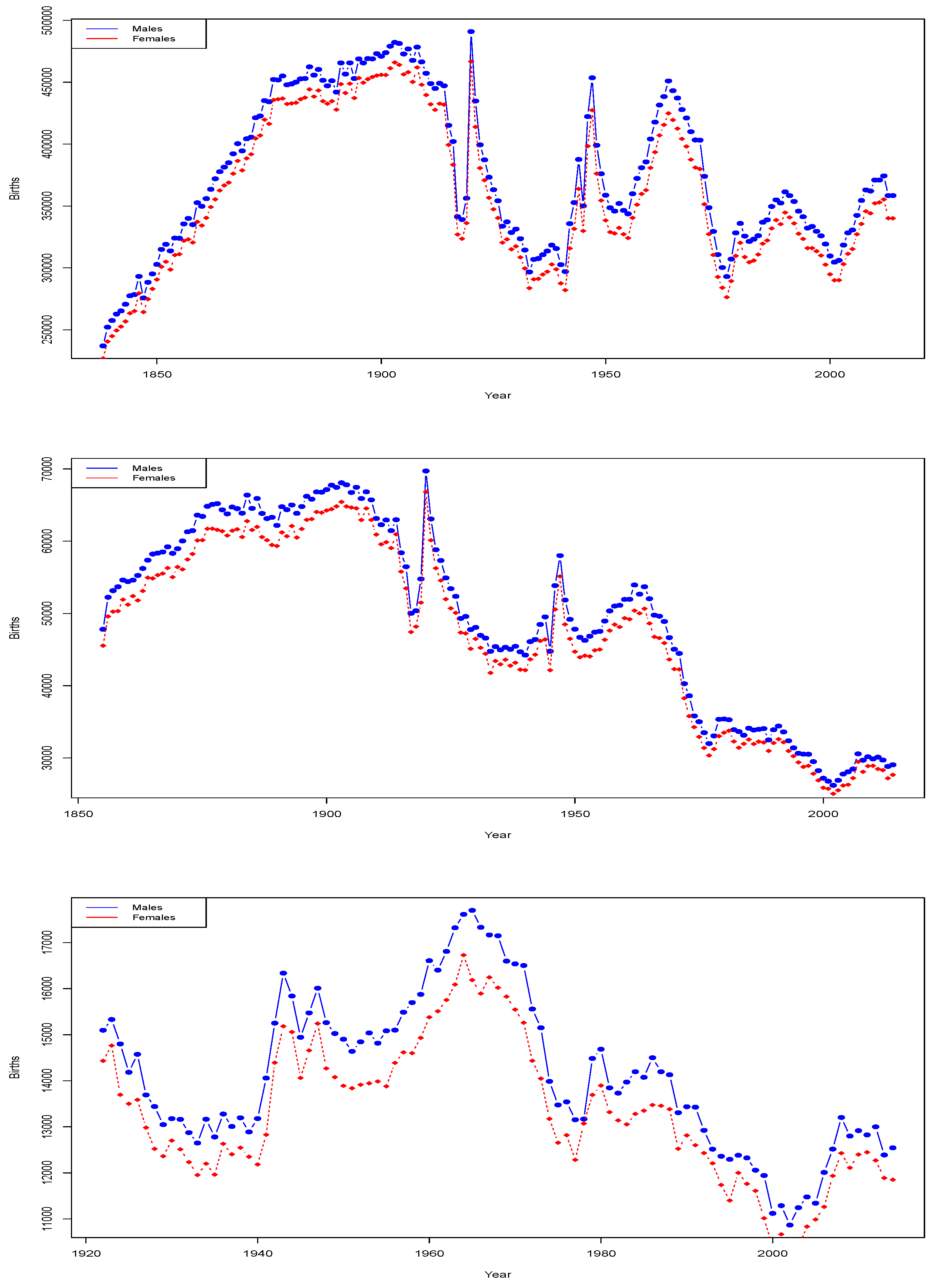
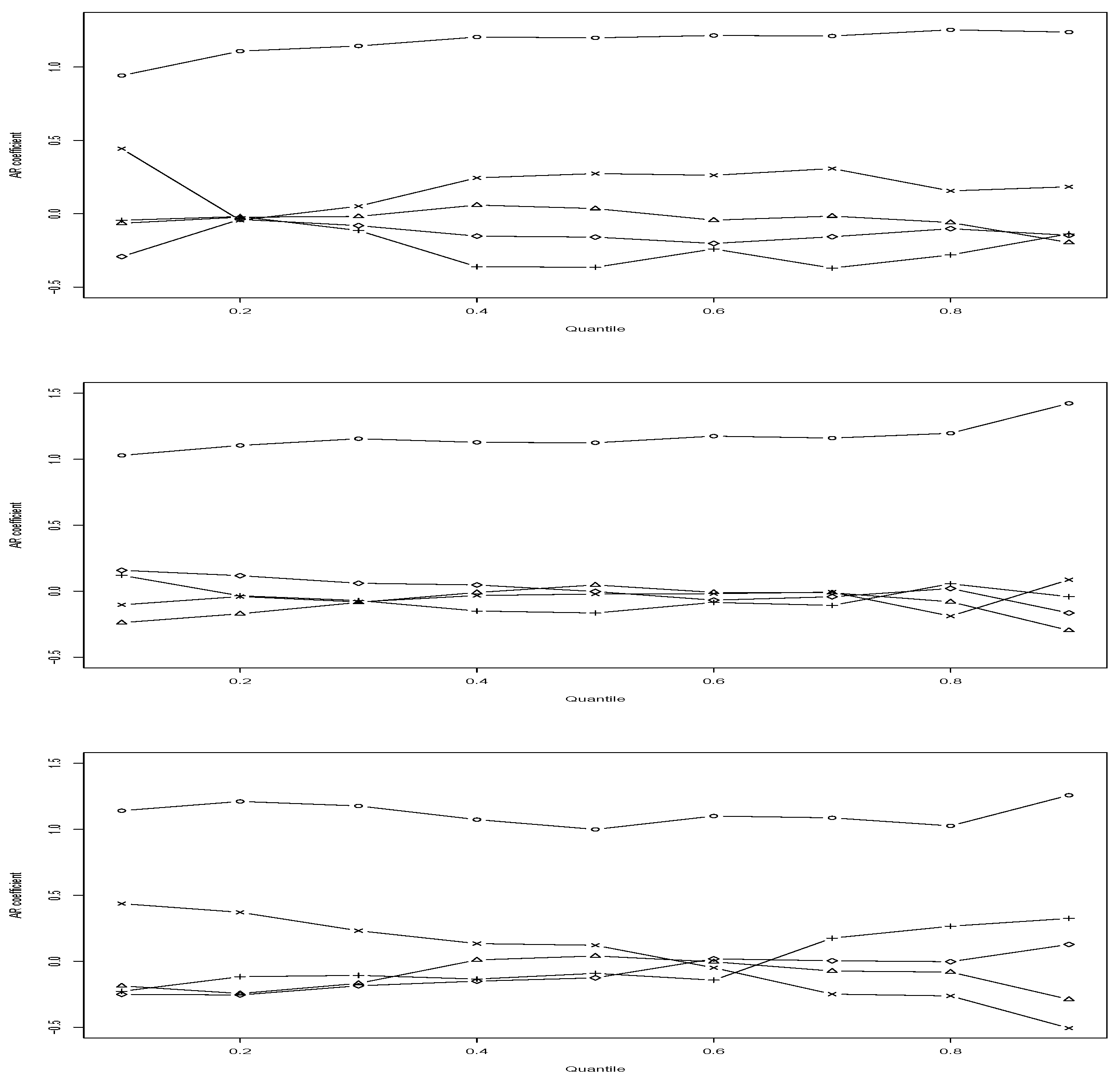
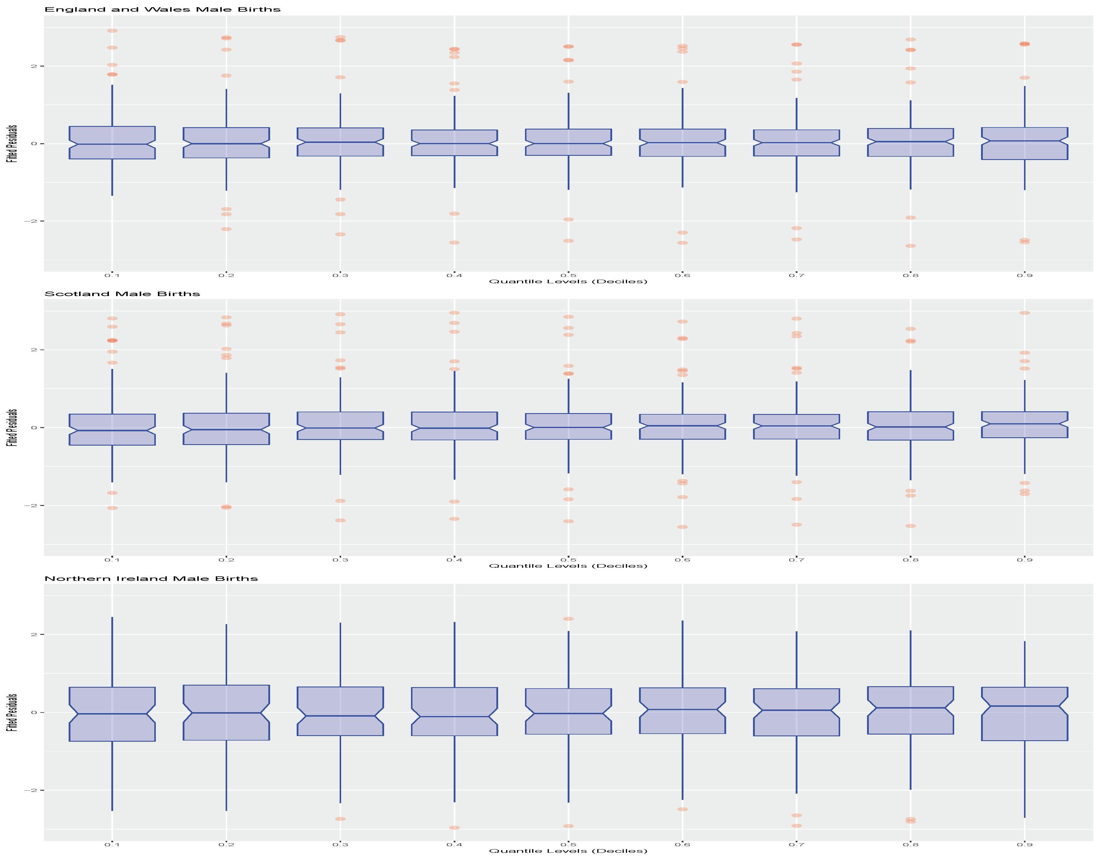
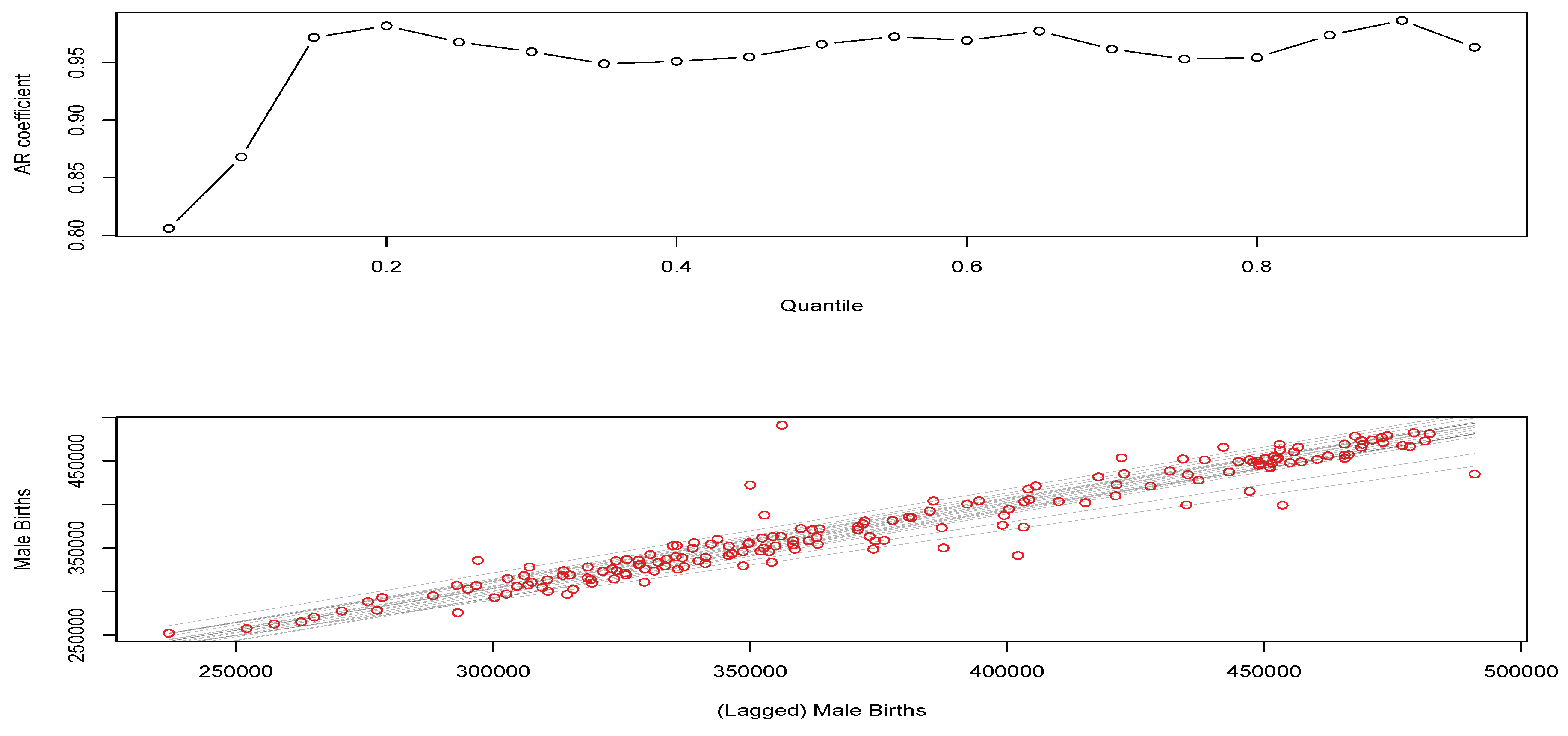
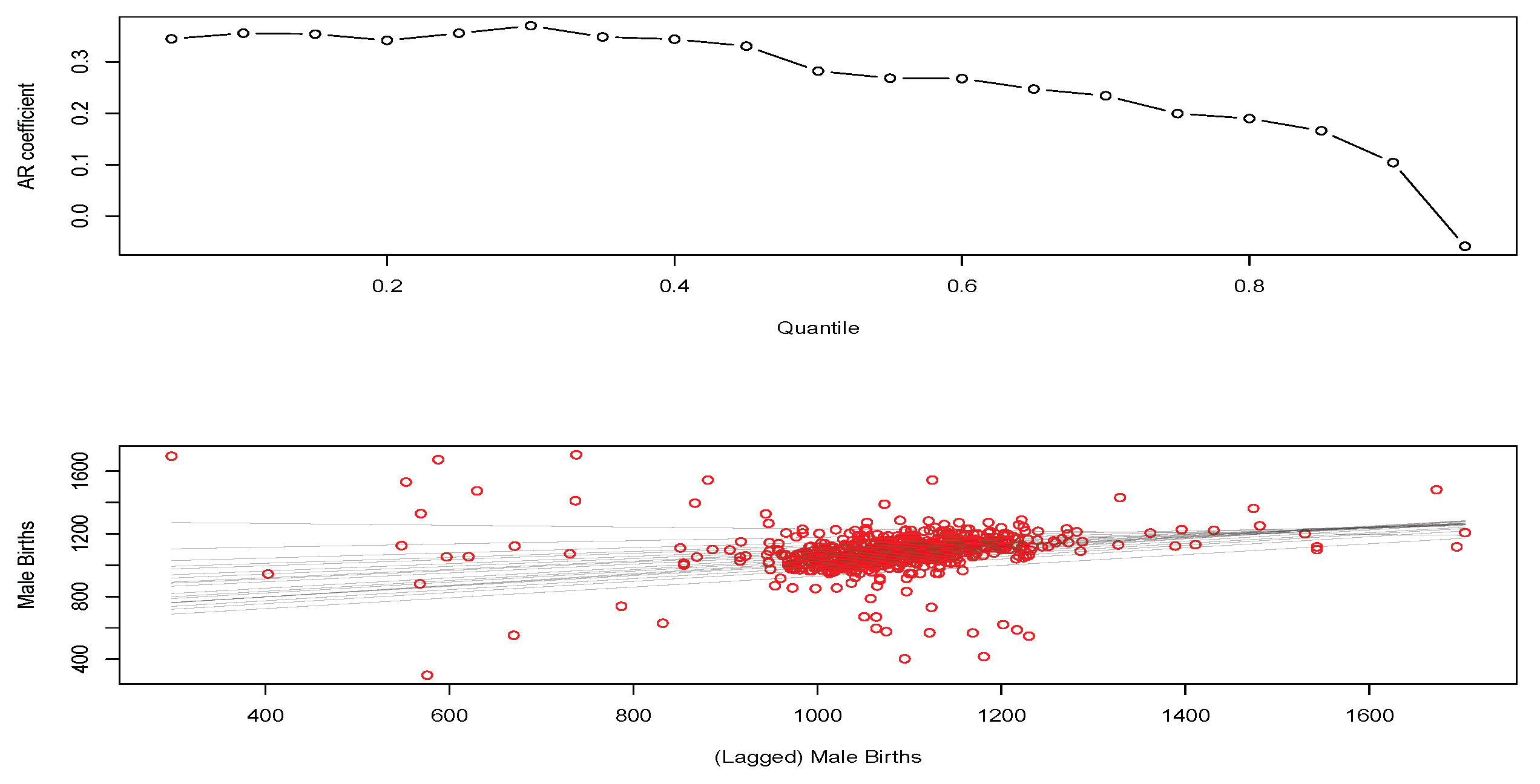
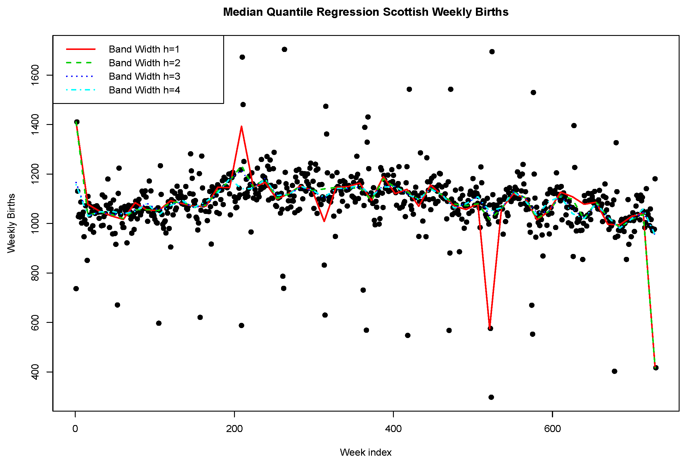
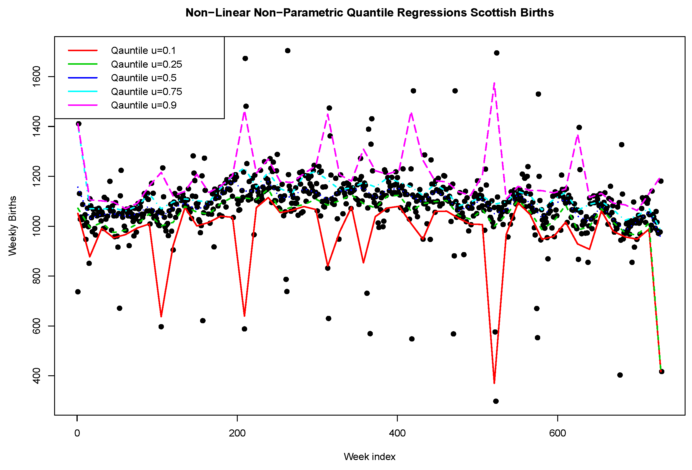
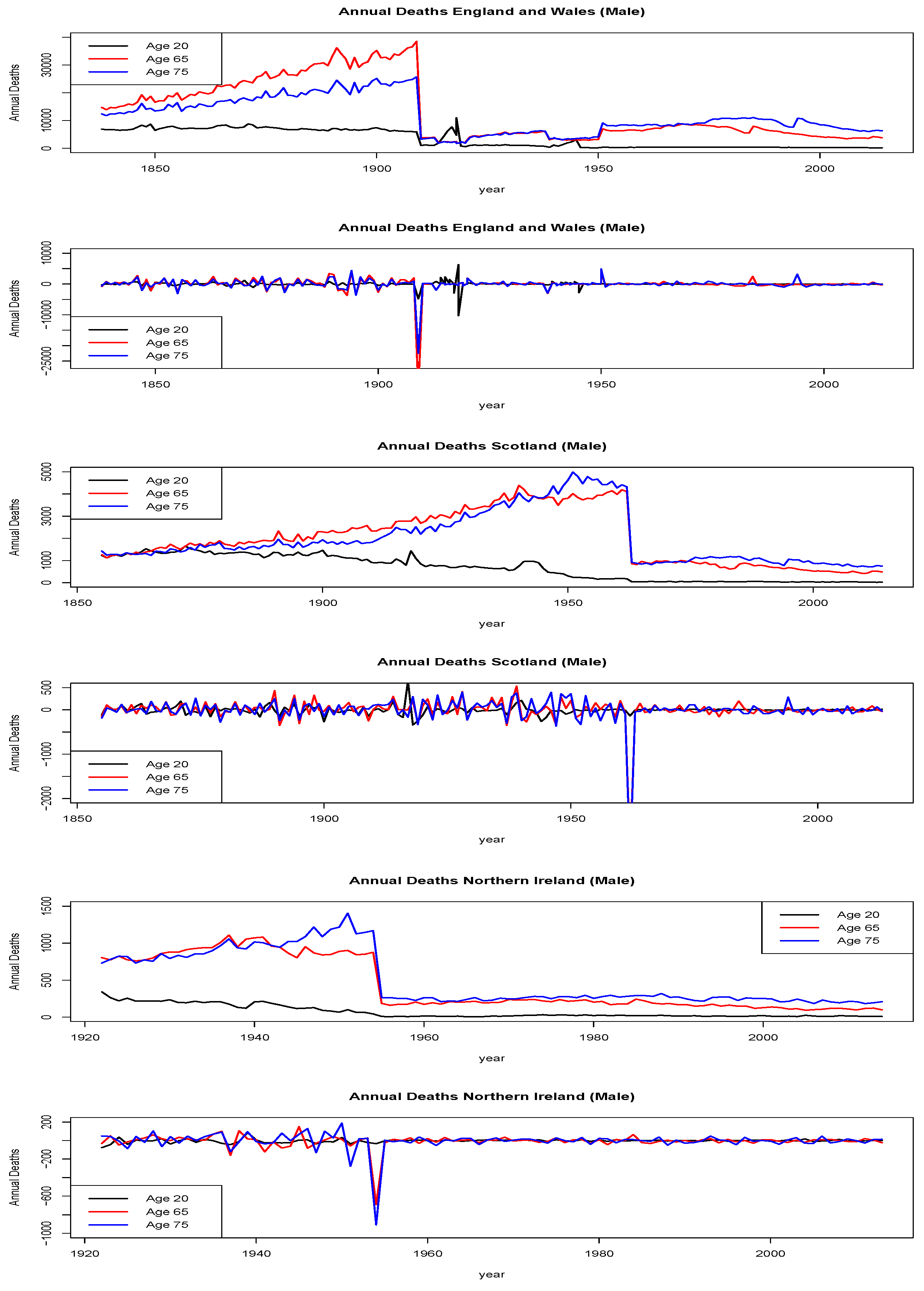
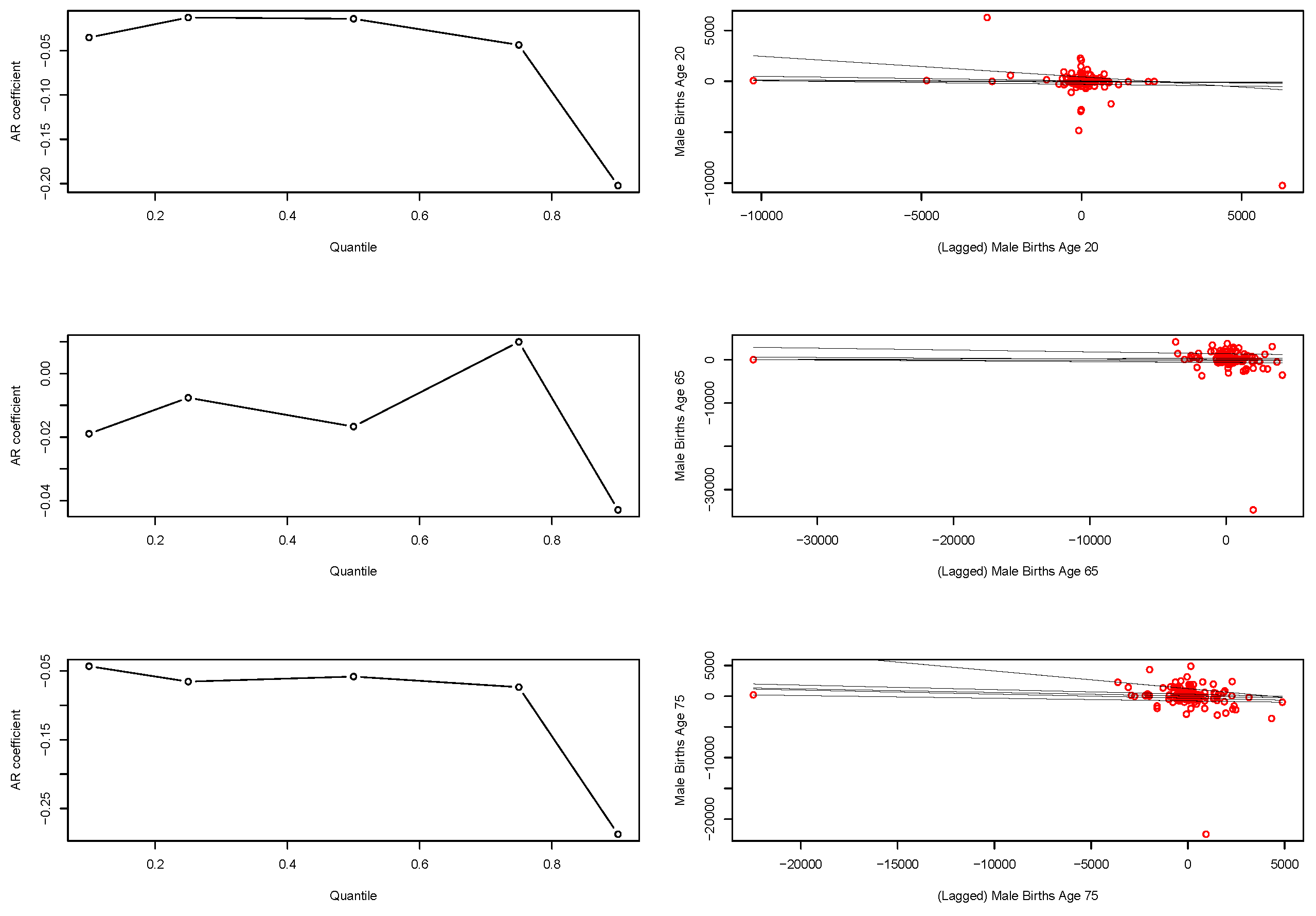
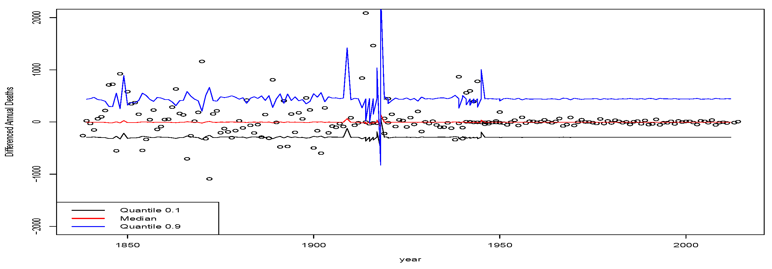
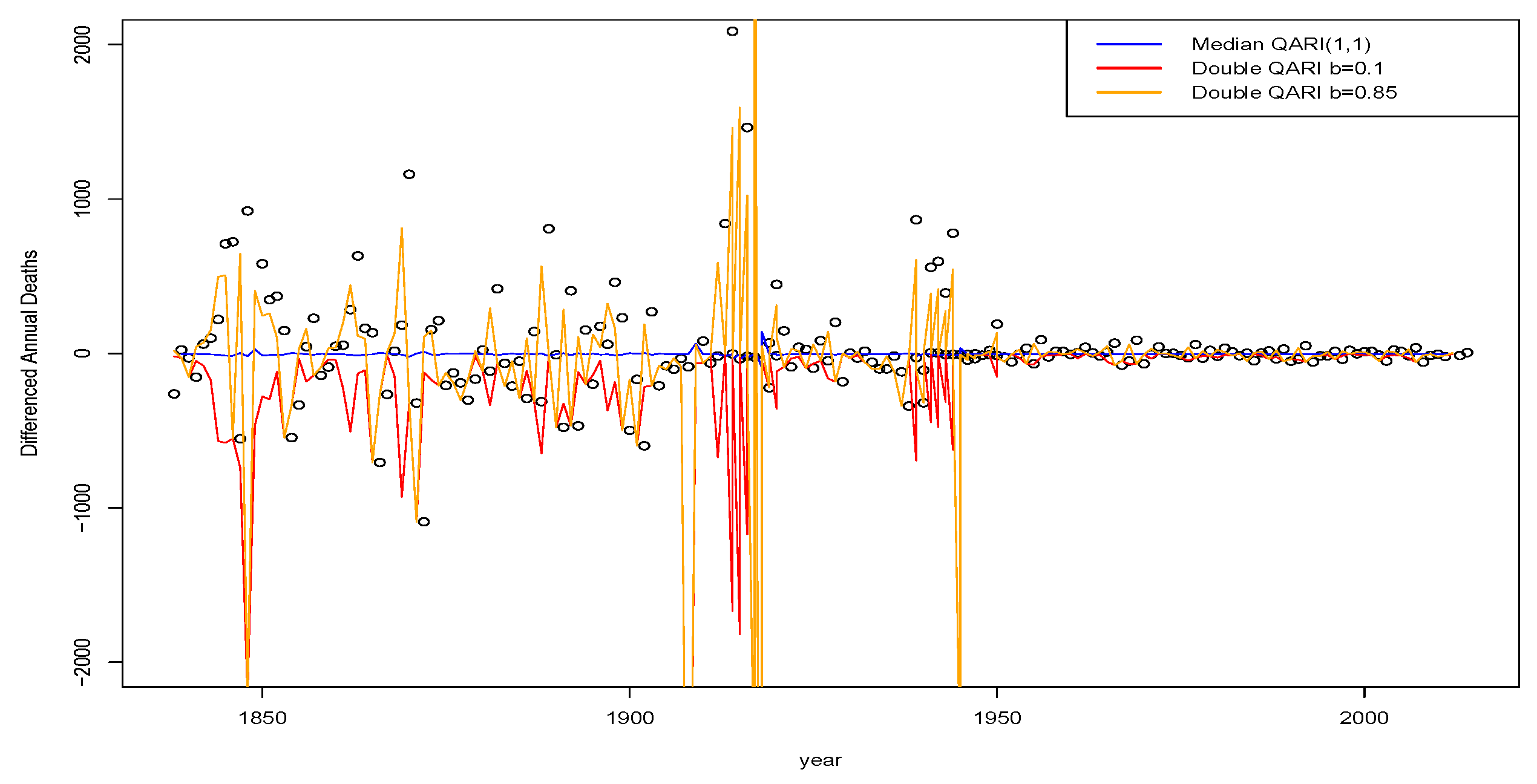
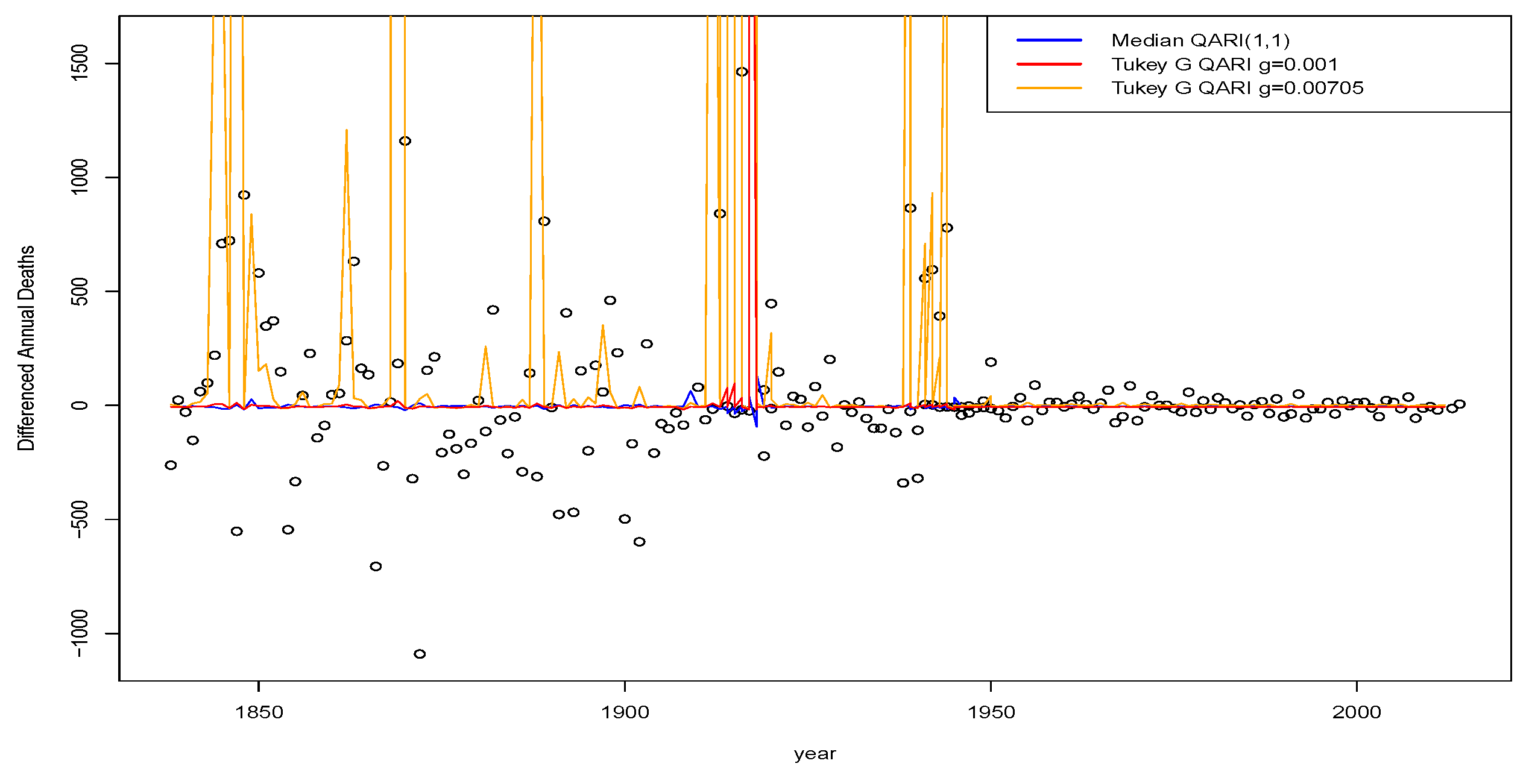
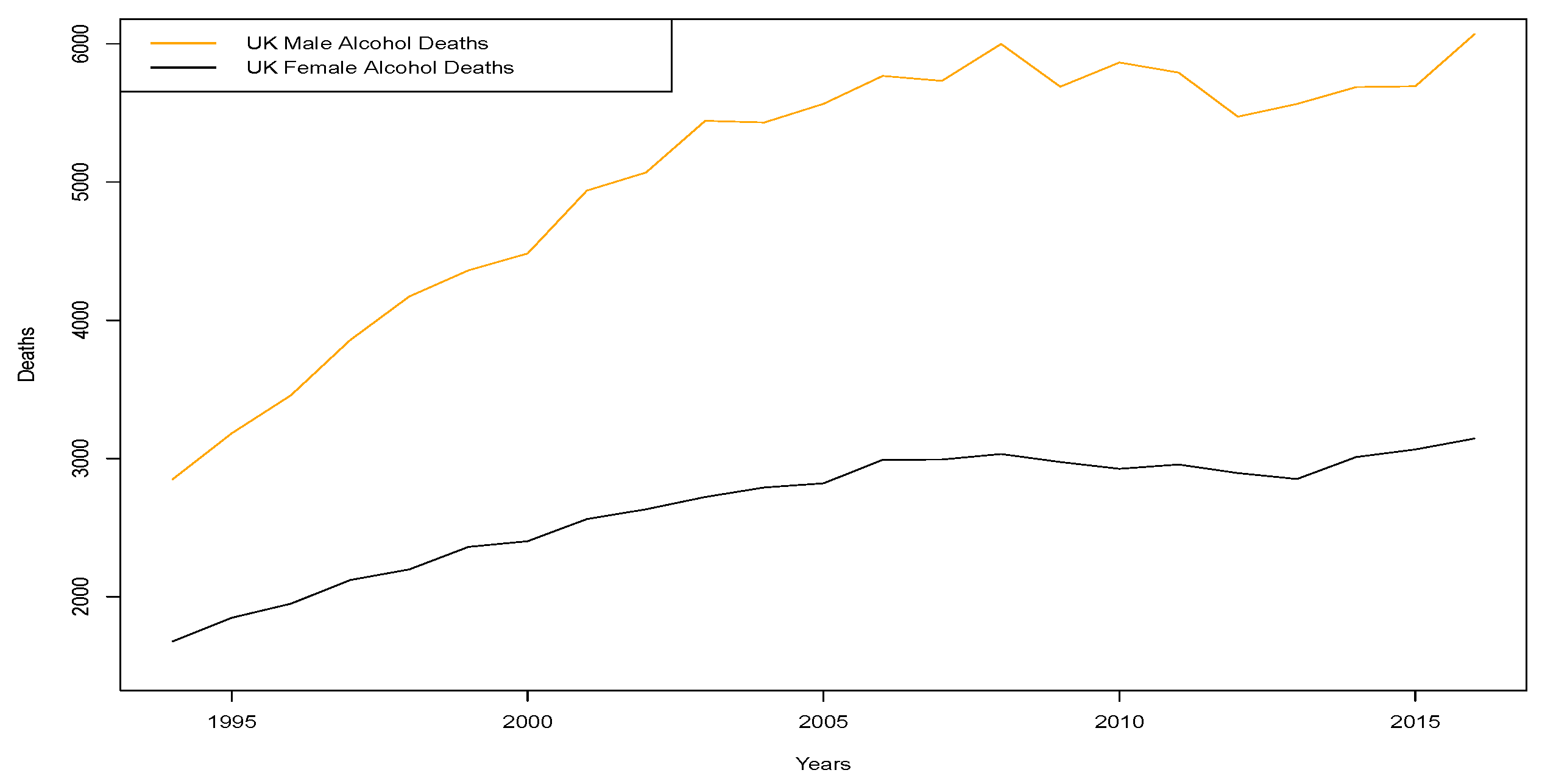
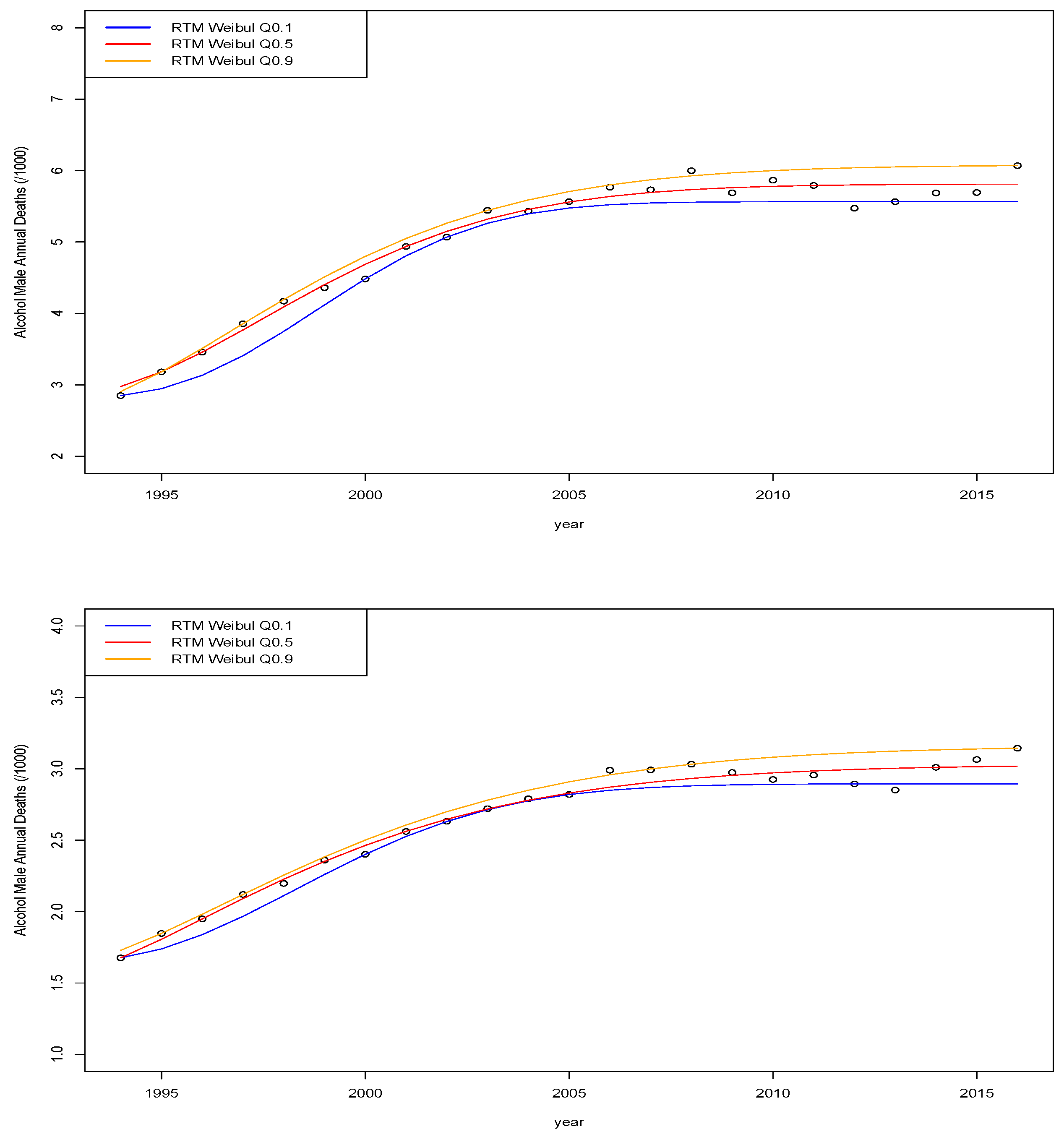
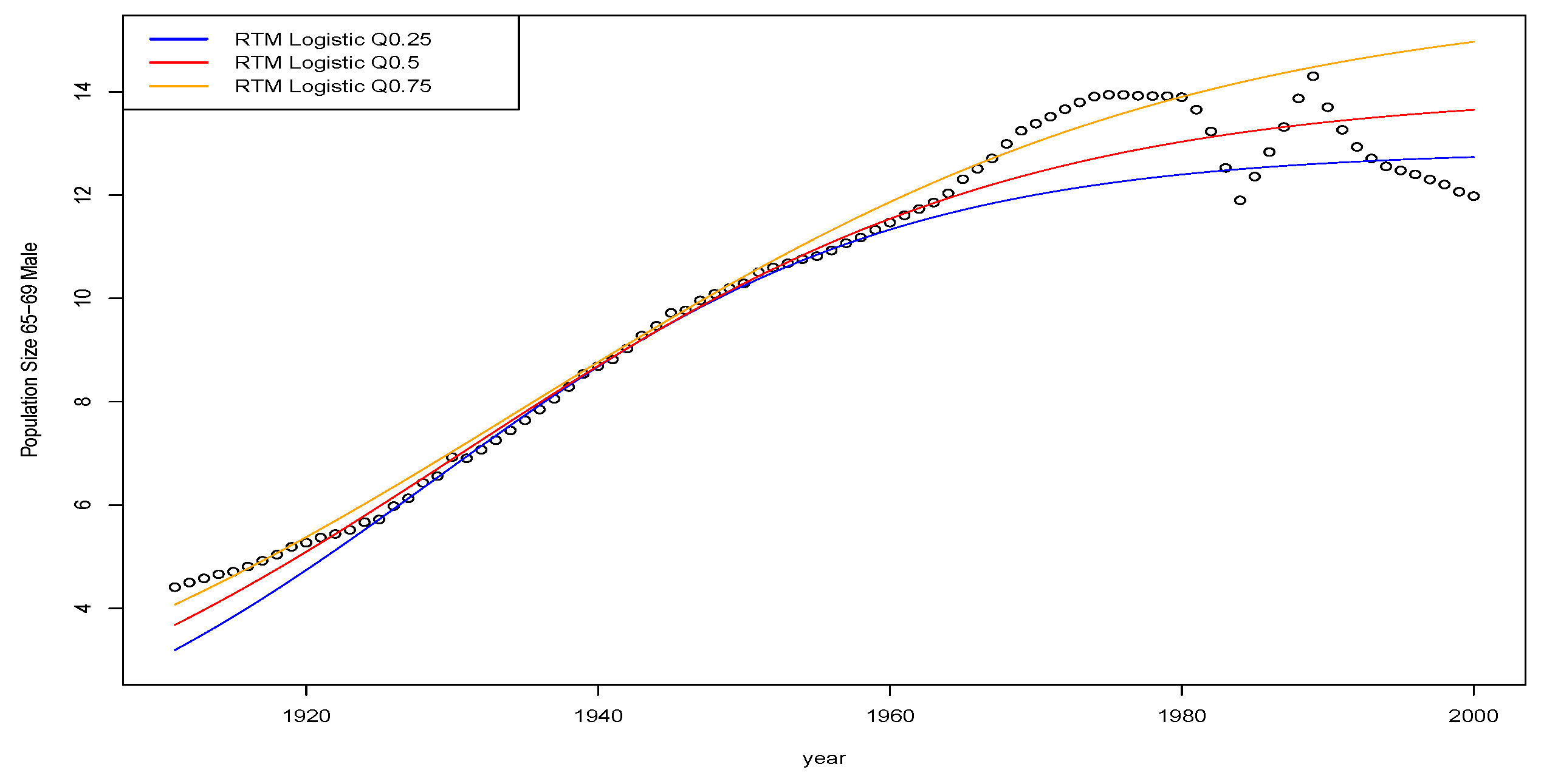10. Conclusions

This manuscript has provided a detailed overview of the different strands of quantile time series regression modelling. Unifying the different approaches in a general modelling framework allows one to treat each key component of a quantile time series model individually. In addition, several properties of special classes of quantile time series model are described and constructed in detail. The paper then concludes with detailed descriptions of different classes of quantile error family and quantile transformation maps that allow for construction of a vast array of flexible quantile time series models. The treatment of estimation is generally not addressed, as the main focus of this overview paper is to address considerations of model construction and the properties of the resulting models.

The illustration of each of the main classes of quantile time series and regression structures explained in the tutorial is then performed in important mortality and demographic data sets for actuarial applications.