A Threshold Type Policy for Trading a Mean-Reverting Asset with Fixed Transaction Costs

Abstract

A mean-reverting model is often used to capture asset price movements fluctuating around its equilibrium. A common strategy trading such mean-reverting asset is to buy low and sell high. However, determining these key levels in practice is extremely challenging. In this paper, we study the optimal trading of such mean-reverting asset with a fixed transaction (commission and slippage) cost. In particular, we focus on a threshold type policy and develop a method that is easy to implement in practice. We formulate the optimal trading problem in terms of a sequence of optimal stopping times. We follow a dynamic programming approach and obtain the value functions by solving the associated HJB equations. The optimal threshold levels can be found by solving a set of quasi-algebraic equations. In addition, a verification theorem is provided together with sufficient conditions. Finally, a numerical example is given to illustrate our results. We note that a complete treatment of this problem was done recently by Leung and associates. Nevertheless, our work was done independently and focuses more on developing necessary optimality conditions.

1. Introduction

This paper is about trading a mean-reverting asset. A common strategy in mean reversion trading is to buy low and sell high. In practice, searching for these key levels is difficult and challenging. In this paper, we focus on mathematical analysis of characterizing these threshold levels.

It is common in financial markets to use a mean-reversion model to capture price movements having the tendency to move towards an “equilibrium”. For example, empirical studies on mean reversion stock returns can be found in (Cowles and Jones 1937), (Fama and French 1988), and (Gallagher and Taylor 2002) among others. Besides stock markets, mean-reversion models are also used for stochastic interest rates (Vasicek 1977; Hull 2003); energy markets (Blanco and Soronow 2001), and stochastic volatility (Hafner and Herwartz 2001).

Mathematical analysis has been used to study trading rules for many years. For instance, (Zhang 2001) studied an optimal selling rule determined by a target price and a stop-loss limit. In (Zhang 2001), these threshold levels are determined by a set of two-point boundary value problems. (Guo and Zhang 2005) considered an optimal selling rule under a regime switching model. They used a smooth-fit technique and obtained the optimal threshold levels. Recent studies combining both the buying and selling decision making can be found in (Dai et al. 2010). In particular, they have established a trend following policy in terms of a conditional probability indicator. They demonstrated that the optimal trading rule can be determined by threshold curves. These curves can be found by solving a set of Hamilton-Jacobi-Bellman (HJB) equations. Similar idea was developed in terms of confidence intervals in (Iwarere and Barmish 2010). Furthermore, (Merhi and Zervos 2007) considered an investment capacity expansion/reduction problem under a geometric Brownian motion market model and followed a dynamic programming approach. A similar problem was treated by (Løkka and Zervos 2013) under a more general market model.

Trading in connection with portfolio management with transaction costs is a class of challenging problems. Research on related optimal consumption and portfolio control can be found in (Øksendal and Sulem 2002) in which they formulated the problem as a combined stochastic control and impulse control problem. They showed that the value function is the unique viscosity solution of the associate QVHJBI. A related problem was considered by (Baccarin and Marazzina 2014) focusing purely on portfolio control. They demonstrated how to best adjust the portfolio so as to maximize an terminal utility function. Further studies along this line can be found in (Baccarin and Marazzina 2016) in which they considered a related problem with solvency constraints. They were able to establish the existence of an impulse policy and provided a numerical method.

Trading under mean reversion models was considered by (Zhang and Zhang 2008). They obtained a threshold type strategy and were able to characterize these two key (low and high) levels in terms of the mean reversion parameters. One key assumption in (Zhang and Zhang 2008) is that the transaction cost associated with each trade is proportional to the current share price. Such proportional cost structure clearly does not work when trading penny stocks. In practice, often a fixed transaction fee is required for trading. This is especially the case when managing not-so-large positions. This issue was successfully addressed in a recent work (Leung et al. 2015). In particular, they studied an optimal multiple trading under a mean reversion model with fixed transaction costs. First, they solved a double stopping problem following a probabilistic approach. They were able to construct the value function directly. Using these results, they infer a similar solution structure for an optimal switching problem in combination with a variational inequality approach. In addition, they have identified the conditions under which the double stopping and switching problem admits the same optimal buying and selling strategies.

In this paper, we study the same problem treated in (Leung et al. 2015). Our main focus was on the variational inequality approach. The main advantage of the variational inequality approach is it mainly involves necessary conditions which is more desirable in applications. In this paper, the objective is to buy and sell the underlying asset sequentially to maximize a discounted reward function. A fixed transaction cost (commission/slippage) is associated with each transaction. We formulate the trading problem in terms of a sequence of stopping times. We follow a dynamic programming approach and obtain the associated HJB equations (quasi-variational inequalities) for the value functions. Using a smooth-fit method, we derive a closed-form solution. The sequence of optimal stopping times can be determined by three threshold levels $x_0$, $x_1$, and $x_2$. Only algebraic equations are needed for these threshold levels. The optimal trading rule can be given in terms of $x_0$, $x_1$, and $x_2$: One should buy when the stock price enters the interval $[e^{x_0},e^{x_1}]$ and sell whenever the price exceeds $e^{x_2}$. In addition, we provide a verification theorem under suitable conditions. We also present a numerical example and demonstrate the dependence of these key levels on various parameters.

This paper is organized as follows. In Section 2, we develop the related mathematical analysis. In particular, in this section, the problem is formulated based on a mean reversion model, relevant properties of the value functions are established, the associated HJB equations and their solutions are obtained, and a verification theorem is provided that guarantees the optimality of our trading policy. In Section 3, we consider a numerical example and study how the threshold levels depend on system parameters. Finally, in Section 4, we conclude the paper by making some remarks.

2. Problem Description and Method

2.1. Formulation of the Optimal Trading Problem

Let $X_t\in \mathrm{I}\mathrm{R}$, $t\ge 0$, denote a mean-reversion process governed by

$$d{X}_t=a(b-X_t)dt+\sigma d{W}_t,X_0=x,$$

(1)

where $W_t$ is a standard Brownian motion, $a>0$ is the rate of reversion, b the equilibrium level, and $\sigma >0$ the volatility. The asset price at time t is given by $S_t=exp\left(X_t\right)$.

Let

$$0\le {\tau }_1\le {\nu }_1\le {\tau }_2\le {\nu }_2\le \cdots$$

(2)

denote a sequence of stopping times where buying is at ${\tau }_n$ and selling is at ${\nu }_n$, $n=1,2,\dots$

We restrict to the case where the net position at any time is either flat (with no share of stock holding) or long (with one share of stock holding). If initially, the net position is long ($i=1$) then one must sell the stock before buying any shares. In this case, the sequence of stopping times is denoted by ${\Lambda }_1=({\nu }_1,{\tau }_2,{\nu }_2,{\tau }_3,\dots )$. Similarly, if the initial net position is flat ($i=0$) then one must first buy a stock before selling any shares. Let ${\Lambda }_0=({\tau }_1,{\nu }_1,{\tau }_2,{\nu }_2,\dots )$ denote the corresponding sequence of stopping times.

Given the initial state $X_0=x$ and initial net position $i=0,1$, let $J_i$ be the reward functions of the decision sequences, ${\Lambda }_0$ and ${\Lambda }_1$:

$$J_i(x,{\Lambda }_i)=\left\{\begin{array}{cc}{\displaystyle E\left\{\sum _{n=1}^{\infty }\left[e^{-\rho {\nu }_n}(S_{{\nu }_n}-K)-e^{-\rho {\tau }_n}(S_{{\tau }_n}+K)\right]\right\},}\hfill & \mathrm{if}i=0,\hfill \\ {\displaystyle E\left\{e^{-\rho {\nu }_1}(S_{{\nu }_1}-K)+\sum _{n=2}^{\infty }\left[e^{-\rho {\nu }_n}(S_{{\nu }_n}-K)-e^{-\rho {\tau }_n}(S_{{\tau }_n}+K)\right]\right\},}\hfill & \mathrm{if}i=1,\hfill \end{array}\right.$$

(3)

where $K>0$ denote the transaction cost per trade, and $\rho >0$ the discount factor.

For simplicity, the term $E{\sum }_{n=1}^{\infty }{\xi }_n$ for random variables ${\xi }_n$ is interpreted as ${lim\; sup}_{N\to \infty }E{\sum }_{n=1}^N{\xi }_n$.

Given the initial net positions $i=0,1$ and initial state $X_0=x$, the corresponding value function

$$V_i\left(x\right)=\underset{{\Lambda }_i}{sup}{J}_i(x,{\Lambda }_i).$$

(4)

Remark 1.

The equalities in (2) allow buying and selling simultaneously. However, due to the existence of positive transaction cost K, these actions cause negative returns and therefore are automatically eliminated by optimality conditions.

Remark 2.

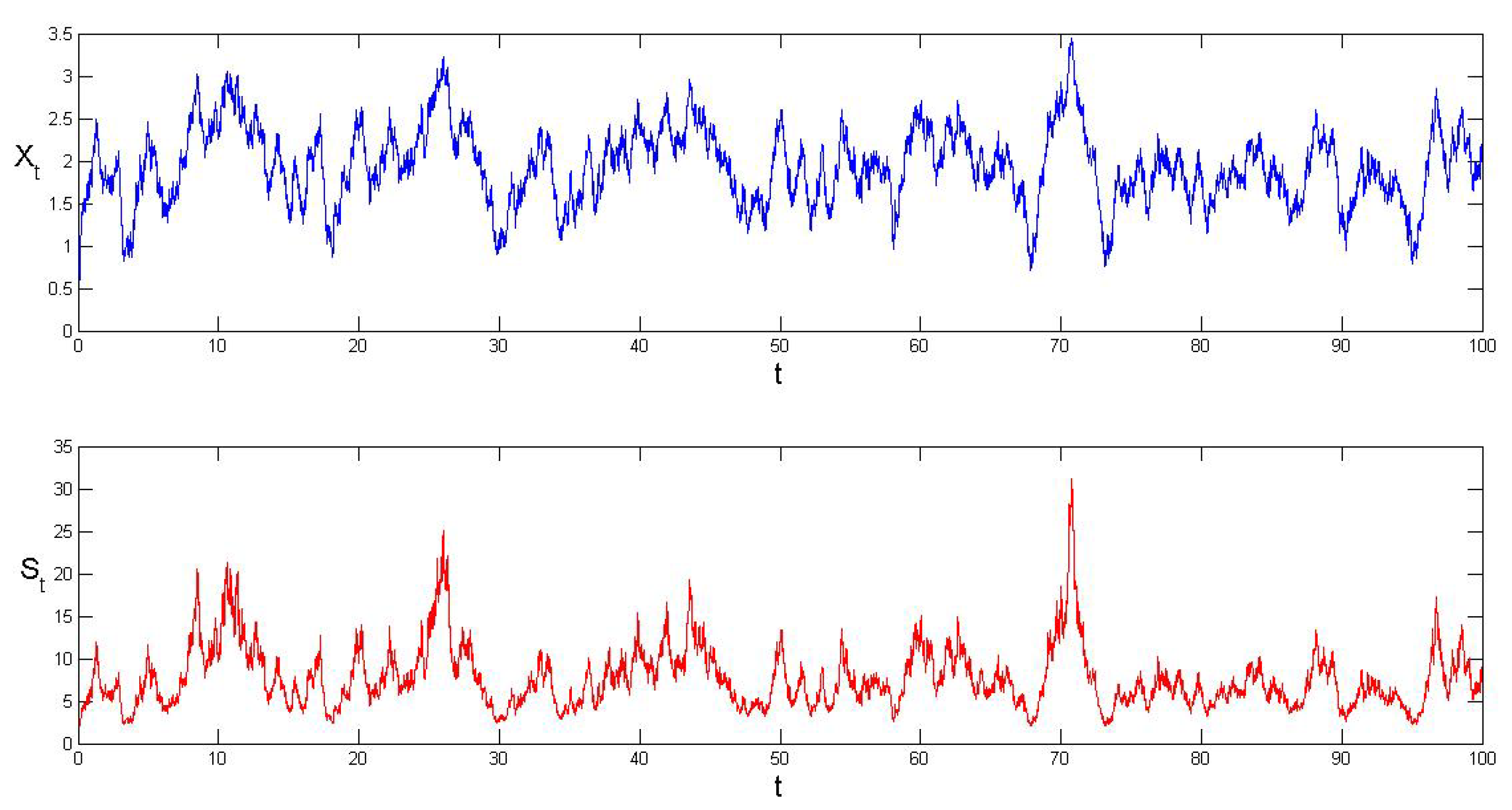
Using the Monte-Carlo, we generate sample paths for $X_t$ and $S_t$ using $a=0.8,b=2,\sigma =0.5$, and $X_0=0.5$. It can be seen in Figure 1 that $X_t$, and $S_t$ fluctuate around the equilibrium level $b=2$, and $e^b=7.388$ respectively.

2.2. Bounds of the Value Functions

Next we establish basic properties of the value functions. We observe that the sequence ${\Lambda }_0=({\tau }_1,{\nu }_1,{\tau }_2,{\nu }_2,\dots )$ can be regarded as a combination of a buy at ${\tau }_1$ and then followed by the sequence of stopping times ${\Lambda }_1=({\nu }_1,{\tau }_2,{\nu }_2,{\tau }_3,\dots )$. Therefore,

$$\begin{array}{cc}\hfill V_0\left(x\right)\ge & {\displaystyle J_0(x,{\Lambda }_0)}\hfill \\ \hfill =& {\displaystyle J_1(X_{{\tau }_1},{\Lambda }_1)-E{e}^{-\rho {\tau }_1}(S_{{\tau }_1}+K).}\hfill \end{array}$$

Setting ${\tau }_1=0$ (recall that $S_t=exp\left(X_t\right)$), and taking supremum over all ${\Lambda }_1$, we get

$$V_0\left(x\right)\ge V_1\left(x\right)-e^x-K.$$

(5)

Similarly,

$$\begin{array}{cc}\hfill V_1\left(x\right)\ge & {\displaystyle J_1(x,{\Lambda }_1)}\hfill \\ \hfill =& {\displaystyle J_0(X_{{\nu }_1},{\Lambda }_0)+E{e}^{-\rho {\nu }_1}(S_{{\nu }_1}-K).}\hfill \end{array}$$

By setting ${\nu }_1=0$, and taking supremum over all ${\Lambda }_0$, we get

$$V_1\left(x\right)\ge V_0\left(x\right)+e^x-K.$$

(6)

In addition, we can establish upper and lower bounds for $V_i\left(x\right)$.

Lemma 1.

There exist constants $K_0$ and $K_1$ such that

$$\begin{array}{c}0\le V_0\left(x\right)\le K_{0}and\hfill \\ V_1\left(x\right)\le e^x+K_1.\hfill \end{array}$$

Proof of Lemma 1.

The lower bound of $V_0$ is clear from the definition. For the upper bound,

$$\begin{array}{cc}\hfill d\left(e^{-\rho t}{S}_t\right)=& {\displaystyle -\rho e^{-\rho t}{S}_{t}dt+e^{-\rho t}(e^{X_t}d{X}_t+\frac{1}{2}{e}^{X_t}{\sigma }^{2}dt)}\hfill \\ \hfill =& {\displaystyle e^{-\rho t}{S}_t(A-a{X}_t)dt+\rho e^{-\rho t}{S}_{t}d{W}_t,}\hfill \end{array}$$

(7)

where $A=\frac{{\sigma }^2}{2}+ab-\rho$. Integrate both sides of the equality in (7) from ${\nu }_n$ to ${\tau }_n$, and then take expectation to get

$$E{e}^{-\rho {\nu }_n}{S}_{{\nu }_n}-E{e}^{-\rho {\tau }_n}{S}_{{\tau }_n}=E{\int }_{{\tau }_n}^{{\nu }_n}{e}^{-\rho t}{e}^{X_t}(A-a{X}_t)dt.$$

Note that the function $e^x(A-ax)$ is bounded above on $\mathrm{I}\mathrm{R}$. Let C be an upper bound. It follows that

$$E{e}^{-\rho {\nu }_n}{S}_{{\nu }_n}-E{e}^{-\rho {\tau }_n}{S}_{{\tau }_n}\le CE{\int }_{{\tau }_n}^{{\nu }_n}{e}^{-\rho t}dt.$$

(8)

Using the definition of $J_0(x,{\Lambda }_0)$, we have

$$\begin{array}{cc}\hfill J_0(x,{\Lambda }_0)\le & {\displaystyle \sum _{n=1}^{\infty }\left(E{e}^{-\rho {\nu }_n}{S}_{{\nu }_n}-E{e}^{-\rho {\tau }_n}{S}_{{\tau }_n}\right)}\hfill \\ \hfill \le & {\displaystyle \sum _{n=1}^{\infty }CE{\int }_{{\tau }_n}^{{\nu }_n}{e}^{-\rho t}dt}\hfill \\ \hfill \le & {\displaystyle CE{\int }_0^{\infty }{e}^{-\rho t}dt=\frac{C}{\rho }:=K_0.}\hfill \end{array}$$

Taking supremum of the inequality over all ${\Lambda }_0$, we obtain $V_0\left(x\right)\le K_0$.

For the bound of $V_1\left(x\right)$, using the definition of $J_1(x,{\Lambda }_1)$, we have

$$J_1(x,{\Lambda }_1)\le J_0(x,{\Lambda }_0)+E{e}^{-\sigma {\rho }_1}(S_{{\nu }_1}-K)\le K_0+E{e}^{-\sigma {\rho }_1}{S}_{{\nu }_1}.$$

Similarly, integrate both sides of the equality in (7) from 0 to ${\nu }_1$, and then take expectation to get

$$E{e}^{-\rho {\nu }_1}{S}_{{\nu }_1}-e^x\le \frac{C}{\rho }.$$

It follows that $J_1(x,{\Lambda }_1)\le 2K_0+e^x$. Taking supremum of the inequality over all ${\Lambda }_1$, we obtain $V_1\left(x\right)\le e^x+K_1,\mathrm{where}{K}_1:=2K_0.$ ☐

2.3. The HJB Equations

In this section, we derive the HJB equations. Formally, the associated HJB equations have the form:

$$\begin{array}{c}min\left\{\rho v_0\left(x\right)-\mathcal{A}{v}_0\left(x\right),v_0\left(x\right)-v_1\left(x\right)+e^x+K\right\}=0,\hfill \\ min\left\{\rho v_1\left(x\right)-\mathcal{A}{v}_1\left(x\right),v_1\left(x\right)-v_0\left(x\right)-e^x+K\right\}=0,\hfill \end{array}$$

(9)

where $\mathcal{A}$ is the generator of $X_t$ given by $\mathcal{A}=a(b-x)\frac{d}{dx}+\frac{{\sigma }^2}{2}\frac{d^2}{d{x}^2}$.

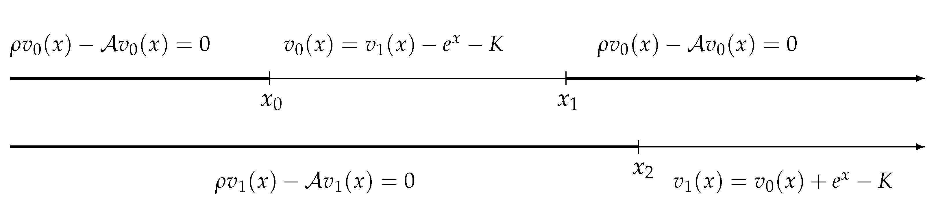
In this paper, we focus on threshold type control policies. Intuitively, if the net position is flat ($i=0$) then one should only buy when the price is low but not much smaller than K (say $X_t$ between $x_0$ and $x_1$). Note that when starting at x in $[x_0,x_1]$, one should buy immediately ($t=0$). In this case, $V_0\left(x\right)=V_1\left(x\right)-e^x-K$. The corresponding continuation region should include $(-\infty ,x_0)\cup (x_1,\infty )$.

On the other hand, if the net position is long ($i=1$) then one should only sell when the price is high (greater than or equal to $x_2$). In this case, $V_1\left(x\right)=V_0\left(x\right)+e^x-K$ and the continuation region should include $(-\infty ,x_2)$. These continuation regions are darkened in Figure 2.

Moreover, one should not establish any new position in continuation regions ($(\rho -\mathcal{A})V_i\left(X_t\right)=0$, $i=0,1$).

In view of these, we can write the HJB equations in terms of these levels:

$$\left\{\begin{array}{cc}{v}_0\left(x\right)\ge v_1\left(x\right)-e^x-K\hfill & \mathrm{on}(-\infty ,x_0)\cup (x_1,\infty ),\hfill \\ v_1\left(x\right)\ge v_0\left(x\right)+e^x-K\hfill & \mathrm{on}(-\infty ,x_2),\hfill \\ (\rho -\mathcal{A})(v_1\left(x\right)-e^x-K)\ge 0\hfill & \mathrm{on}(x_0,x_1),\hfill \\ (\rho -\mathcal{A})(v_0\left(x\right)+e^x-K)\ge 0\hfill & \mathrm{on}(x_2,\infty ),\hfill \end{array}\right.$$

(10)

and

$$\left\{\begin{array}{cc}{v}_0\left(x\right)=v_1\left(x\right)-e^x-K\hfill & \mathrm{on}[x_0,x_1],\hfill \\ v_1\left(x\right)=v_0\left(x\right)+e^x-K\hfill & \mathrm{on}[x_2,\infty ),\hfill \\ (\rho -\mathcal{A})v_0\left(x\right)=0\hfill & \mathrm{on}(-\infty ,x_0]\cup [x_1,\infty ),\hfill \\ (\rho -\mathcal{A})v_1\left(x\right)=0\hfill & \mathrm{on}(-\infty ,x_2].\hfill \end{array}\right.$$

(11)

We next examine the conditions in (10) and (11) on intervals $(-\infty ,x_0)$, $(x_0,x_1)$, $(x_1,x_2)$, and $(x_2,\infty )$.

On $(-\infty ,x_0)$ and $(x_1,x_2)$, it requires the first two inequalities of (10), i.e., $|v_1\left(x\right)-v_0\left(x\right)-e^x|\le K.$

On $(x_0,x_1)$, it requires the second and third inequalities of (10). Note that on this interval, the second inequality is automatically satisfied. Using $(\rho -\mathcal{A})v_1\left(x\right)=0$, the third inequality can be simplified to $f\left(x\right):=e^x(-ax+ab-\rho +{\sigma }^2/2)-\rho K\ge 0.$ Then $f^{\prime }\left(x\right)=e^x(-ax+ab-a+{\sigma }^2/2-\rho )$. This implies $f\left(x\right)$ has the only local and absolute maximum at $x_{max}=(ab-a+{\sigma }^2/2-\rho )/a$. Therefore, it is necessary $f\left(x_0\right)\ge 0$ and $f\left(x_1\right)\ge 0$.

On $(x_2,\infty )$, it requires the first and last inequality of (10). Note that on this interval, the first inequality is automatically satisfied. Using $(\rho -\mathcal{A})v_0\left(x\right)=0$, the last inequality can be simplified to $e^x(ax-ab+\rho -{\sigma }^2/2)-\rho K\ge 0.$ Equivalently, $g\left(x\right):=ax-ab+\rho -{\sigma }^2/2-\rho K{e}^{-x}\ge 0.$ Then $g^{\prime }\left(x\right)=a+\rho K{e}^{-x}\ge 0$. Therefore, it is necessary $g\left(x_2\right)\ge 0$.

2.4. Solutions of the HJB Equations

We will obtain the threshold levels $(x_0,x_1,x_2)$ by solving the HJB equations in (9). We first solve the equations $\rho v_i\left(x\right)-\mathcal{A}{v}_i\left(x\right)=0$ with $i=0,1$.

Let

$$\left\{\begin{array}{c}{\displaystyle {\varphi }_1\left(x\right)={\int }_0^{\infty }\eta \left(t\right)e^{-\kappa (b-x)t}dt,}\hfill \\ {\displaystyle {\varphi }_2\left(x\right)={\int }_0^{\infty }\eta \left(t\right)e^{\kappa (b-x)t}dt,}\hfill \end{array}\right.$$

where $\kappa =\sqrt{2a}/\sigma$, $\lambda =\rho /a$, and $\eta \left(t\right)=t^{\lambda -1}exp\left(-t^2/2\right)$. Then the general solution of $\rho v_i\left(x\right)-\mathcal{A}{v}_i\left(x\right)=0$ is given by a linear combination of these functions (details can be found in (Eloe et al. 2008)).

Note that ${\varphi }_1\left(\infty \right)=\infty$ and ${\varphi }_2(-\infty )=\infty$. We will derive $v_i\left(x\right),i=1,2$, on each continuation region.

First, consider the interval $(x_1,\infty )$. Suppose $v_0\left(x\right)=A_1{\varphi }_1\left(x\right)+A_2{\varphi }_2\left(x\right)$, for some $A_1$ and $A_2$. By Lemma 1, $v_0\left(\infty \right)$ should be bounded above. This implies $A_1=0$ and so $v_0\left(x\right)=A_2{\varphi }_2\left(x\right)$.

On the interval $(-\infty ,x_0)$, suppose $v_0\left(x\right)=B_1{\varphi }_1\left(x\right)+B_2{\varphi }_2\left(x\right)$, for some $B_1$ and $B_2$. By Lemma 1, $v_0(-\infty )$ should be bounded above. This implies $B_2=0$ and hence $v_0\left(x\right)=B_1{\varphi }_1\left(x\right)$.

On the interval $(-\infty ,x_2)$, suppose $v_1\left(x\right)=C_1{\varphi }_1\left(x\right)+C_2{\varphi }_2\left(x\right)$, for some $C_1$ and $C_2$. By Lemma 1, $v_0(-\infty )$ should be bounded above. This implies $C_2=0$ and therefore $v_1\left(x\right)=C_1{\varphi }_1\left(x\right)$.

Since $v_i\left(x\right),i=1,2,$ are twice continuously differentiable on their continuation region, we can follow the smooth-fit method. In particular, it requires $v_0\left(x\right)$ to be continuously differentiable at $x_0$ and $x_1$, and $v_1\left(x\right)$ to be continuously differentiable at $x_2$. Therefore,

$$\left\{\begin{array}{c}{B}_1{\varphi }_1\left(x_0\right)=C_1{\varphi }_1\left(x_0\right)-e^{x_0}-K,\hfill \\ B_1{\varphi }_1^{\prime }\left(x_0\right)=C_1{\varphi }_1^{\prime }\left(x_0\right)-e^{x_0},\hfill \end{array}\right.$$

$$\left\{\begin{array}{c}{A}_2{\varphi }_2\left(x_1\right)=C_1{\varphi }_1\left(x_1\right)-e^{x_1}-K,\hfill \\ A_2{\varphi }_2^{\prime }\left(x_1\right)=C_1{\varphi }_1^{\prime }\left(x_1\right)-e^{x_1},\hfill \end{array}\right.$$

and

$$\left\{\begin{array}{c}{C}_1{\varphi }_1\left(x_2\right)=A_2{\varphi }_2\left(x_2\right)+e^{x_2}-K,\hfill \\ C_1{\varphi }_1^{\prime }\left(x_2\right)=A_2{\varphi }_2^{\prime }\left(x_2\right)+e^{x_2}.\hfill \end{array}\right.$$

Let

$$\Phi \left(x\right)=\left(\begin{array}{cc}{\displaystyle {\varphi }_1\left(x\right)}& {\displaystyle {\varphi }_2\left(x\right)}\\ {\displaystyle {\varphi }_1^{\prime }\left(x\right)}& {\displaystyle {\varphi }_2^{\prime }\left(x\right)}\end{array}\right).$$

Note that the matrix $\Phi \left(x\right)$ is invertible for all x because its determinant is less than zero by direct computation.

The systems above are equivalent to

$$\left\{\begin{array}{c}(B_1-C_1){\varphi }_1\left(x_0\right)=-e^{x_0}-K\hfill \\ (B_1-C1){\varphi }_1^{\prime }\left(x_0\right)=-e^{x_0},\hfill \end{array}\right.$$

(12)

$$\Phi \left(x_1\right)\left(\begin{array}{c}{C}_1\\ -A_2\end{array}\right)=\left(\begin{array}{c}{e}^{x_1}+K\\ e^{x_1}\end{array}\right),$$

(13)

$$\Phi \left(x_2\right)\left(\begin{array}{c}{C}_1\\ -A_2\end{array}\right)=\left(\begin{array}{c}{e}^{x_2}-K\\ e^{x_2}\end{array}\right).$$

(14)

It follows from (13) and (14) that

$$\left(\begin{array}{c}{C}_1\\ -A_2\end{array}\right)={\Phi }^{-1}\left(x_1\right)\left(\begin{array}{c}{e}^{x_1}+K\\ e^{x_1}\end{array}\right)={\Phi }^{-1}\left(x_2\right)\left(\begin{array}{c}{e}^{x_2}-K\\ e^{x_2}\end{array}\right).$$

(15)

In (12), divide the first equation by the second to get ${\displaystyle \frac{{\varphi }_1\left(x_0\right)}{{\varphi }_1^{\prime }\left(x_0\right)}=\frac{e^{x_0}+K}{e^{x_0}}}$. This implies

$${\varphi }_1\left(x_0\right)e^{x_0}={\varphi }_1^{\prime }\left(x_0\right)(e^{x_0}+K).$$

(16)

Solve (15) to get $x_1$ and $x_2$, and then obtain $A_2$ and $C_1$. Also, solve (16) to get $x_0$, and then obtain $B_1$ from (12). Hence, the values function are determined by

$$v_0\left(x\right)=\left\{\begin{array}{cc}{B}_1{\varphi }_1\left(x\right)\hfill & \mathrm{on}(-\infty ,x_0),\hfill \\ C_1{\varphi }_1\left(x\right)-e^x-K\hfill & \mathrm{on}[x_0,x_1),\hfill \\ A_2{\varphi }_2\left(x\right)\hfill & \mathrm{on}[x_1,\infty ).\hfill \end{array}\right.$$

(17)

$$v_1\left(x\right)=\left\{\begin{array}{cc}{C}_1{\varphi }_1\left(x\right)\hfill & \mathrm{on}(-\infty ,x_2),\hfill \\ A_2{\varphi }_2\left(x\right)+e^x-K\hfill & \mathrm{on}[x_2,\infty ).\hfill \end{array}\right.$$

(18)

Additionally, due to the existence of the transaction cost, if the stock was bought at $S_1=e^{x_1}$ and sold at $S_2=e^{x_2}$ then it requires that $e^{x_2}-K>e^{x_1}+K$. Equivalently,

$$e^{x_2}-e^{x_1}>2K.$$

(19)

2.5. A Verification Theorem

We will summarize the analysis in Section 2.3 in a Verification Theorem, and show that the solution $v_i\left(x\right)$, $i=0,1$, of Equation (9) is equal to the value functions $V_i\left(x\right)$, $i=0,1$, respectively, and sequences of optimal stopping times can be characterized by the triple $(x_0,x_1,x_2)$.

Theorem 1.

Recall $f\left(x\right)=e^x(-ax+ab-\rho +{\sigma }^2/2)-\rho K$ and $g\left(x\right)=ax-ab+\rho -{\sigma }^2/2-\rho K{e}^{-x}$. Let $(x_0,x_1,x_2)$ be a solution to (15) and(16)satisfying $e^{x_2}-e^{x_1}>2K$, and $f\left(x_0\right)$, $f\left(x_1\right)$, and $g\left(x_2\right)$ are all non-negative. Let $A_2,B_1,C_1$ be constants given by (15) and (12). Let

$$\left\{\begin{array}{c}{v}_0\left(x\right)=\left\{\begin{array}{cc}{\displaystyle B_1{\varphi }_1\left(x\right)}\hfill & on(-\infty ,x_0),\hfill \\ {\displaystyle C_1{\varphi }_1\left(x\right)-e^x-K}\hfill & on[x_0,x_1),\hfill \\ {\displaystyle A_2{\varphi }_2\left(x\right)}\hfill & on[x_1,\infty ).\hfill \end{array}\right.\hfill \\ v_1\left(x\right)=\left\{\begin{array}{cc}{\displaystyle C_1{\varphi }_1\left(x\right)}\hfill & on(-\infty ,x_2),\hfill \\ {\displaystyle A_2{\varphi }_2\left(x\right)+e^x-K}\hfill & on[x_2,\infty ).\hfill \end{array}\right.\hfill \end{array}\right.$$

Assume $v_0\left(x_2\right)\ge 0$, and $|v_1\left(x\right)-v_0\left(x\right)-e^x|\le K$ on $(-\infty ,x_0)\cup (x_1,x_2)$. Then

$$v_i\left(x\right)=V_i\left(x\right),i=0,1.$$

Moreover, if initially $i=0$, let ${\Lambda }_0^{*}=({\tau }_1^{*},{\nu }_1^{*},{\tau }_2^{*},{\nu }_2^{*},\dots ),$ where the stopping times ${\tau }_1^{*}=inf\{t\ge 0:X_t\in [x_0,x_1]\}$, ${\nu }_n^{*}=inf\{t\ge {\tau }_n^{*}:X_t=x_2\}$, and ${\tau }_{n+1}^{*}=inf\{t>{\nu }_n^{*}:X_t\in [x_0,x_1]\}$ for $n\ge 1$. Similarly, if initially $i=1$, let ${\Lambda }_1^{*}=({\nu }_1^{*},{\tau }_2^{*},{\nu }_2^{*},{\tau }_3^{*},\dots ),$ where the stopping times ${\nu }_1^{*}=inf\{t\ge 0:X_t\ge x_2\}$, ${\tau }_n^{*}=inf\{t>{\nu }_{n-1}^{*}:X_t\in [x_0,x_1]\}$, and ${\nu }_n^{*}=inf\{t\ge {\tau }_n^{*}:X_t=x_2\}$ for $n\ge 2$.

Then ${\Lambda }_0^{*}$ and ${\Lambda }_1^{*}$ are optimal.

The following lemmas will be used in the proof of Theorem 1.

Lemma 2.

For any stopping times ${\theta }_1$ and ${\theta }_2$, if $0\le {\theta }_1\le {\theta }_2$, a.s., and $\rho v_i\left(X_t\right)-\mathcal{A}{v}_i\left(X_t\right)\ge 0$, for all $t\in [{\theta }_1,{\theta }_2]$, for $i=0,1$, then

$$E{e}^{-\rho {\theta }_1}{v}_i\left(X_{{\theta }_1}\right)\ge E{e}^{-\rho {\theta }_2}{v}_i\left(X_{{\theta }_2}\right).$$

In particular, if ${\theta }_1=0$, ${\theta }_2=\tau \ge 0$, and $X_0=x$ then $v_i\left(x\right)\ge E{e}^{-\rho \tau }{v}_i\left(X_{\tau }\right).$

The equalities happen when $\rho v_i\left(X_t\right)-\mathcal{A}{v}_i\left(X_t\right)=0$ for all $t\in [{\theta }_1,{\theta }_2]$.

Proof of Lemma 2.

For $i=0,1$,

$$\begin{array}{ccc}\hfill d\left(e^{-\rho t}{v}_i\left(X_t\right)\right)& =& {\displaystyle -\rho e^{-\rho t}{v}_i\left(X_t\right)dt+e^{-\rho t}\left\{\left[a(b-X_t)v_i^{\prime }\left(X_t\right)+\frac{1}{2}{\sigma }^2{v}_i^{″}\left(X_t\right)\right]dt+\sigma v^{\prime }\left(X_t\right)d{W}_t\right\}}\hfill \\ & =\hfill & {\displaystyle e^{-\rho t}(-\rho +\mathcal{A})v_i\left(X_t\right)dt+\sigma e^{-\rho t}{v}_i^{\prime }\left(X_t\right)d{W}_t.}\hfill \end{array}$$

Integrate both sides of this equation from ${\theta }_1$ to ${\theta }_2$, and then take expectation to obtain

$$E{e}^{-\rho {\theta }_2}{v}_i\left(X_{{\theta }_2}\right)-E{e}^{-\rho {\theta }_1}{v}_i\left(X_{{\theta }_1}\right)=E\left[{\int }_{{\theta }_1}^{{\theta }_2}-e^{-\rho t}(\rho -\mathcal{A})v_i\left(X_t\right)dt\right].$$

(20)

(20) and the hypothesis $\rho v_i\left(X_t\right)-\mathcal{A}{v}_i\left(X_t\right)\ge 0$ for all $t\in [{\theta }_1,{\theta }_2]$ give

$$E{e}^{-\rho {\theta }_1}{v}_i\left(X_{{\theta }_1}\right)\ge E{e}^{-\rho {\theta }_2}{v}_i\left(X_{{\theta }_2}\right).$$

Set ${\theta }_1=0,{\theta }_2=\tau$ to obtain

$$v_i\left(x\right)\ge E{e}^{-\rho \tau }{v}_i\left(X_{\tau }\right).$$

Moreover, if $\rho v_i\left(X_t\right)-\mathcal{A}{v}_i\left(X_t\right)=0$ for all $t\in [{\theta }_1,{\theta }_2]$ then (20) gives the equalities. ☐

Lemma 3.

If the position is $i=0$ and ${\Lambda }_0=({\tau }_1,{\nu }_1,{\tau }_2,{\nu }_2,\dots )$ then for all $N\ge 1$,

$$E{e}^{-\rho {\tau }_1}{v}_0\left(X_{{\tau }_1}\right)\ge E{e}^{-\rho {\nu }_N}{v}_0\left(X_{{\nu }_N}\right)+E\sum _{n=1}^N\left[e^{-\rho {\nu }_n}(S_{{\nu }_n}-K)-e^{-\rho {\tau }_n}(S_{{\tau }_n}+K)\right].$$

Similarly, if the position is $i=1$ and ${\Lambda }_1=({\nu }_1,{\tau }_2,{\nu }_2,{\tau }_3,\dots )$ then for all $N\ge 2$,

$$E{e}^{-\rho {\nu }_1}{v}_1\left(X_{{\nu }_1}\right)\ge E{e}^{-\rho {\nu }_N}{v}_0\left(X_{{\nu }_N}\right)+E{e}^{-\rho {\nu }_1}(S_{{\nu }_1}-K)+E\sum _{n=2}^N\left[e^{-\rho {\nu }_n}(S_{{\nu }_n}-K)-e^{-\rho {\tau }_n}(S_{{\tau }_n}+K)\right].$$

Proof of Lemma 3.

Since $v_i,i=1,2$ are solutions of the HJB equations in (9), we have for all $t\ge 0$,

$$\begin{array}{c}\hfill v_0\left(X_t\right)\ge v_1\left(X_t\right)-e^{X_t}-K,\\ \hfill v_1\left(X_t\right)\ge v_0\left(X_t\right)+e^{X_t}-K.\end{array}$$

(21)

It follows, for the position $i=0$, that

$$\begin{array}{cc}\hfill E{e}^{-\rho {\tau }_1}{v}_0\left(X_{{\tau }_1}\right)\ge & {\displaystyle E{e}^{-\rho {\tau }_1}\left(v_1\left(X_{{\tau }_1}\right)-S_{{\tau }_1}-K\right)}\hfill \\ \hfill \ge & {\displaystyle E{e}^{-\rho {\nu }_1}{v}_1\left(X_{{\nu }_1}\right)-E{e}^{-\rho {\tau }_1}(S_{{\tau }_1}+K)}\hfill \\ \hfill \ge & {\displaystyle E{e}^{-\rho {\nu }_1}(v_0\left(X_{{\nu }_1}\right)+S_{{\nu }_1}-K)-E{e}^{-\rho {\tau }_1}(S_{{\tau }_1}+K)}\hfill \\ \hfill \ge & {\displaystyle E{e}^{-\rho {\tau }_2}{v}_0\left(X_{{\tau }_2}\right)+E\left[e^{-\rho {\nu }_1}(S_{{\nu }_1}-K)-e^{-\rho {\tau }_1}(S_{{\tau }_1}+K)\right].}\hfill \end{array}$$

In the expressions above, the second line uses Lemma 2 for ${\tau }_1\le {\nu }_1$. The third line uses (21). The last line uses Lemma 2 for ${\nu }_1\le {\tau }_2$.

Similarly,

$$E{e}^{-\rho {\tau }_2}{v}_0\left(X_{{\tau }_2}\right)\ge E{e}^{-\rho {\nu }_2}{v}_0\left(X_{{\nu }_2}\right)+E\left[e^{-\rho {\nu }_2}(S_{{\nu }_2}-K)-e^{-\rho {\tau }_2}(S_{{\tau }_2}+K)\right].$$

(22)

Continue this way to obtain the first inequality of Lemma 3:

$${\displaystyle E{e}^{-\rho {\tau }_1}{v}_0\left(X_{{\tau }_1}\right)\ge E{e}^{-\rho {\nu }_N}{v}_0\left(X_{{\nu }_N}\right)+E\sum _{n=1}^N\left[e^{-\rho {\nu }_n}(S_{{\nu }_n}-K)-e^{-\rho {\tau }_n}(S_{{\tau }_n}+K)\right]\mathrm{for}\mathrm{all}N\ge 1.}$$

For the second inequality, we use similar computations for the position $i=1$.

$$\begin{array}{cc}\hfill E{e}^{-\rho {\nu }_1}{v}_1\left(X_{{\nu }_1}\right)\ge & {\displaystyle E{e}^{-\rho {\nu }_1}\left(v_0\left(X_{{\nu }_1}\right)+S_{{\nu }_1}-K\right)}\hfill \\ \hfill \ge & {\displaystyle E{e}^{-\rho {\tau }_2}(v_0\left(X_{{\tau }_2}\right)+E{e}^{-\rho {\nu }_1}(S_{{\nu }_1}-K)}\hfill \\ \hfill \ge & {\displaystyle E{e}^{-\rho {\nu }_2}{v}_0\left(X_{{\nu }_2}\right)+E\left[e^{-\rho {\nu }_2}(S_{{\nu }_2}-K)-e^{-\rho {\tau }_2}(S_{{\tau }_2}+K)\right]+E{e}^{-\rho {\nu }_1}(S_{{\nu }_1}-K).}\hfill \end{array}$$

Continue this way to obtain the second inequality of Lemma 3. ☐

Lemma 4.

If the position is $i=0$ and ${\Lambda }_0^{*}=({\tau }_1^{*},{\nu }_1^{*},{\tau }_2^{*},{\nu }_2^{*},\dots )$ is defined as in Theorem 1, then for all $N\ge 1$,

$$E{e}^{-\rho {\tau }_1^{*}}{v}_0\left(X_{{\tau }_1^{*}}\right)=E{e}^{-\rho {\nu }_N^{*}}{v}_0\left(X_{{\nu }_N^{*}}\right)+E\sum _{n=1}^N\left[e^{-\rho {\nu }_n^{*}}(S_{{\nu }_n^{*}}-K)-e^{-\rho {\tau }_n^{*}}(S_{{\tau }_n^{*}}+K)\right].$$

Similarly, if the position is $i=1$ and ${\Lambda }_1^{*}=({\nu }_1^{*},{\tau }_2^{*},{\nu }_2^{*},{\tau }_3^{*},\dots )$ is defined as in Theorem 1, then for all $N\ge 2$,

$$E{e}^{-\rho {\nu }_1^{*}}{v}_1\left(X_{{\nu }_1^{*}}\right)=E{e}^{-\rho {\nu }_N^{*}}{v}_0\left(X_{{\nu }_N^{*}}\right)+E{e}^{-\rho {\nu }_1^{*}}(S_{{\nu }_1^{*}}-K)+E\sum _{n=2}^N\left[e^{-\rho {\nu }_n^{*}}(S_{{\nu }_n^{*}}-K)-e^{-\rho {\tau }_n^{*}}(S_{{\tau }_n^{*}}+K)\right].$$

Proof of Lemma 4.

Since $v_i$, $i=1,2$ are solutions of the HJB equations in (9), they have to satisfy (11), i.e.,

$$\left\{\begin{array}{cc}{v}_0\left(x\right)=v_1\left(x\right)-e^x-K\hfill & \mathrm{on}[x_0,x_1],\hfill \\ v_1\left(x\right)=v_0\left(x\right)+e^x-K\hfill & \mathrm{on}[x_2,\infty ),\hfill \\ (\rho -\mathcal{A})v_0\left(x\right)=0\hfill & \mathrm{on}(-\infty ,x_0]\cup [x_1,\infty ),\hfill \\ (\rho -\mathcal{A})v_1\left(x\right)=0\hfill & \mathrm{on}(-\infty ,x_2].\hfill \end{array}\right.$$

It has been shown by (Zhang and Zhang 2008) that ${\tau }_n^{*}<\infty$, and ${\nu }_n^{*}<\infty$ a.s. for $n\ge 1$.

Now consider the position $i=0$. Note that $X_{{\tau }_1^{*}}\in [x_0,x_1]$. Hence,

$$E{e}^{-\rho {\tau }_1^{*}}{v}_0\left(X_{{\tau }_1^{*}}\right)=E{e}^{-\rho {\tau }_1^{*}}{v}_1\left(X_{{\tau }_1^{*}}\right)-E{e}^{-\rho {\tau }_1^{*}}(S_{{\tau }_1^{*}}+K).$$

Note that $X_t\in (-\infty ,x_2]$ for all $t\in [{\tau }_1^{*},{\nu }_1^{*}]$ and $X_{{\nu }_1^{*}}=x_2$. This implies $(\rho -\mathcal{A})v_1\left(X_t\right)=0$ for all $t\in [{\tau }_1^{*},{\nu }_1^{*}]$ and $v_1\left(X_{{\nu }_1^{*}}\right)=v_0\left(X_{{\nu }_1^{*}}\right)+e^{X_{{\nu }_1^{*}}}-K$. Lemma 2 implies

$$\begin{array}{cc}\hfill E{e}^{-\rho {\tau }_1^{*}}{v}_1\left(X_{{\tau }_1^{*}}\right)=& {\displaystyle E{e}^{-\rho {\nu }_1^{*}}{v}_1\left(X_{{\nu }_1^{*}}\right)}\hfill \\ \hfill =& {\displaystyle E{e}^{-\rho {\nu }_1^{*}}{v}_0\left(X_{{\nu }_1^{*}}\right)+E{e}^{-\rho {\nu }_1^{*}}(S_{{\nu }_1^{*}}-K).}\hfill \end{array}$$

Therefore,

$$E{e}^{-\rho {\tau }_1^{*}}{v}_1\left(X_{{\tau }_1^{*}}\right)=E{e}^{-\rho {\nu }_1^{*}}{v}_0\left(X_{{\nu }_1^{*}}\right)+E\left[e^{-\rho {\nu }_1^{*}}(S_{{\nu }_1^{*}}-K)-e^{-\rho {\tau }_1^{*}}(S_{{\tau }_1^{*}}+K)\right].$$

Note that $X_t\in [x_1,\infty )$ for all $t\in [{\nu }_1^{*},{\tau }_2^{*}]$. This implies $(\rho -\mathcal{A})v_0\left(X_t\right)=0$ for all $t\in [{\nu }_1^{*},{\tau }_2^{*}]$. Lemma 2 implies $E{e}^{-\rho {\nu }_1^{*}}{v}_0\left(X_{{\nu }_1^{*}}\right)=E{e}^{-\rho {\tau }_2^{*}}{v}_0\left(X_{{\tau }_2^{*}}\right)$.

Similarly,

$$E{e}^{-\rho {\tau }_2^{*}}{v}_0\left(X_{{\tau }_2^{*}}\right)=E{e}^{-\rho {\nu }_2^{*}}{v}_0\left(X_{{\nu }_2^{*}}\right)+E\left[e^{-\rho {\nu }_2^{*}}(S_{{\nu }_2^{*}}-K)-e^{-\rho {\tau }_2^{*}}(S_{{\tau }_2^{*}}+K)\right].$$

(23)

Continue the procedure to obtain

$$E{e}^{-\rho {\tau }_1^{*}}{v}_1\left(X_{{\tau }_1^{*}}\right)=E{e}^{-\rho {\nu }_N^{*}}{v}_0\left(X_{{\nu }_N^{*}}\right)+E\sum _{n=1}^N\left[e^{-\rho {\nu }_n^{*}}(S_{{\nu }_n^{*}}-K)-e^{-\rho {\tau }_n^{*}}(S_{{\tau }_n^{*}}+K)\right]\mathrm{for}\mathrm{all}N\ge 1.$$

For the second equality, we use similar computations for the position $i=1$ as follows.

Note that $X_{{\nu }_1^{*}}\in [x_2,\infty )$. Hence,

$$E{e}^{-\rho {\nu }_1^{*}}{v}_1\left(X_{{\nu }_1^{*}}\right)=E{e}^{-\rho {\nu }_1^{*}}{v}_0\left(X_{{\nu }_1^{*}}\right)+E{e}^{-\rho {\nu }_1^{*}}(S_{{\nu }_1^{*}}-K).$$

Note also that $X_t\in [x_1,\infty )$ for all $t\in [{\nu }_1^{*},{\tau }_2^{*}]$. This implies $(\rho -\mathcal{A})v_0\left(X_t\right)=0$ for all $t\in [{\nu }_1^{*},{\tau }_2^{*}]$. Lemma 2 implies $E{e}^{-\rho {\nu }_1^{*}}{v}_0\left(X_{{\nu }_1^{*}}\right)=E{e}^{-\rho {\tau }_2^{*}}{v}_0\left(X_{{\tau }_2^{*}}\right)$. Use (23) to obtain

$$E{e}^{-\rho {\nu }_1^{*}}{v}_0\left(X_{{\nu }_1^{*}}\right)=E{e}^{-\rho {\nu }_2^{*}}{v}_0\left(X_{{\nu }_2^{*}}\right)+E\left[e^{-\rho {\nu }_2^{*}}(S_{{\nu }_2^{*}}-K)-e^{-\rho {\tau }_2^{*}}(S_{{\tau }_2^{*}}+K)\right].$$

Similarly, $E{e}^{-\rho {\nu }_2^{*}}{v}_0\left(X_{{\nu }_2^{*}}\right)=E{e}^{-\rho {\nu }_3^{*}}{v}_0\left(X_{{\nu }_3^{*}}\right)+E\left[e^{-\rho {\nu }_3^{*}}(S_{{\nu }_3^{*}}-K)-e^{-\rho {\tau }_3^{*}}(S_{{\tau }_3^{*}}+K)\right].$

Continue the procedure to obtain the second equality. ☐

Proof of Theorem 1.

The proof consists of two steps. In the first step, we show that $v_i\left(x\right)\ge J_i(x,{\Lambda }_i)$ for all ${\Lambda }_i$. Then in the second step, we show that $v_i\left(x\right)=J_i(x,{\Lambda }_i^{*})$. Therefore, $v_i\left(x\right)=V_i\left(x\right)$, and ${\Lambda }_i^{*}$ is optimal.

For the first step, first note that

$$v_0\left(X_{{\nu }_N}\right)=v_0\left(x_2\right)\mathrm{for}{\nu }_N\in {\Lambda }_0,N\ge 1,$$

and

$$v_0\left(X_{{\nu }_N}\right)=v_0\left(x_2\right)\mathrm{for}{\nu }_N\in {\Lambda }_1,N\ge 2.$$

In view of Lemma 3 and the assumption $v_0\left(x_2\right)\ge 0$, we have

$$\begin{array}{cc}\hfill E{e}^{-\rho {\tau }_1}{v}_0\left(X_{{\tau }_1}\right)\ge & {\displaystyle E\sum _{n=1}^N\left[e^{-\rho {\nu }_n}(S_{{\nu }_n}-K)-e^{-\rho {\tau }_n}(S_{{\tau }_n}+K)\right]\mathrm{for}N\ge 1,\mathrm{and}}\hfill \\ \hfill E{e}^{-\rho {\nu }_1}{v}_1\left(X_{{\nu }_1}\right)\ge & {\displaystyle E{e}^{-\rho {\nu }_1}(S_{{\nu }_1}-K)+E\sum _{n=2}^N\left[e^{-\rho {\nu }_n}(S_{{\nu }_n}-K)-e^{-\rho {\tau }_n}(S_{{\tau }_n}+K)\right]\mathrm{for}N\ge 2.}\hfill \end{array}$$

Moreover, since $v_i,i=0,1$, satisfy the quasi-variational inequalities in (9), $\rho v_i\left(X_t\right)-\mathcal{A}{v}_i\left(X_t\right)\ge 0$ for all $t\ge 0$. Let $X_0=x$. Use Lemma 2 to obtain

$$v_0\left(x\right)\ge E{e}^{-\rho {\tau }_1}{v}_0\left(X_{{\tau }_1}\right)\mathrm{and}{v}_1\left(x\right)\ge E{e}^{-\rho {\nu }_1}{v}_1\left(X_{{\nu }_1}\right).$$

Sending $N\to \infty$, we obtain $v_0\left(x\right)\ge J_0(x,{\Lambda }_0)$ for all ${\Lambda }_0$, and $v_1\left(x\right)\ge J_1(x,{\Lambda }_1)$ for all ${\Lambda }_1$. This implies that $v_0\left(x\right)\ge V_0\left(x\right)$ and $v_1\left(x\right)\ge V_1\left(x\right)$.

For the second step, we establish the equalities. Note that $v_0\in C^2(\mathrm{I}\mathrm{R}\backslash \{x_0,x_1\})$, $v_1\in C^2(\mathrm{I}\mathrm{R}\backslash \left\{x_2\right\})$, and both $v_0$ and $v_1$ are in $C^1\left(\mathrm{I}\mathrm{R}\right)$.

Note also that if the position is $i=0$ then $X_t\in (-\infty ,x_0]\cup [x_1,\infty )$ for all $t\in [0,{\tau }_1^{*}]$, which implies $(\rho -\mathcal{A})v_0\left(X_t\right)=0$ for all $t\in [0,{\tau }_1^{*}]$.

Similarly, if the position is $i=1$ then $X_t\in (-\infty ,x_2]$ for all $t\in [0,{\nu }_1^{*}]$, which implies $(\rho -\mathcal{A})v_1\left(X_t\right)=0$ for all $t\in [0,{\nu }_1^{*}]$.

Using Lemma 2, we get $v_0\left(x\right)=E{e}^{-\rho {\tau }_1^{*}}{v}_0\left(X_{{\tau }_1^{*}}\right)\mathrm{and}{v}_1\left(x\right)=E{e}^{-\rho {\nu }_1^{*}}{v}_0\left(X_{{\nu }_1^{*}}\right).$

In view of Lemma 4, it remains to show $E{e}^{-\rho {\nu }_N^{*}}{v}_0\left(X_{{\nu }_N^{*}}\right)\to 0$.

Note that $X_{{\nu }_N^{*}}=x_2$ for all $N\ge 0$, therefore, $v_0\left(X_{{\nu }_N^{*}}\right)=v_0\left(x_2\right)$.

Thus, it suffices to show $E{e}^{-\rho {\nu }_N^{*}}\to 0$ as $N\to \infty$. To this end, note that $v_0\left(x_2\right)\ge 0$ by assumption, so let $N\to \infty$ in the first equation of Lemma 4 to obtain

$$\begin{array}{cc}\hfill v_0\left(x\right)\ge & {\displaystyle \sum _{n=1}^{\infty }E\left[e^{-\rho {\nu }_n^{*}}(S_{{\nu }_n^{*}}-K)-e^{-\rho {\tau }_n^{*}}(S_{{\tau }_n^{*}}+K)\right]}\hfill \\ \hfill =& {\displaystyle -E{e}^{-\rho {\tau }_1^{*}}(S_{{\tau }_1^{*}}+K)+\sum _{n=1}^{\infty }E\left[e^{-\rho {\nu }_n^{*}}(S_{{\nu }_n^{*}}-K)-e^{-\rho {\tau }_{n+1}^{*}}(S_{{\tau }_{n+1}^{*}}+K)\right]}\hfill \\ \hfill \ge & {\displaystyle -E{e}^{-\rho {\tau }_1^{*}}(S_{{\tau }_1^{*}}+K)+\sum _{n=1}^{\infty }E\left[S_{{\nu }_n^{*}}-S_{{\tau }_{n+1}^{*}}-2K\right]e^{-\rho {\nu }_n^{*}}}\hfill \\ \hfill =& {\displaystyle -E{e}^{-\rho {\tau }_1^{*}}(S_{{\tau }_1^{*}}+K)+(e^{x_2}-e^{x_1}-2K)\sum _{n=1}^{\infty }E{e}^{-\rho {\nu }_n^{*}}.}\hfill \end{array}$$

Furthermore, $e^{x_2}-e^{x_1}-2K>0$ by assumption and ${\tau }_1^{*}<\infty$ a.s. (Zhang and Zhang 2008). Also, it can be seen from the definition of $v_0\left(x\right)$ in Theorem 1 that $v_0\left(x\right)$ is bounded. These imply the convergence of ${\displaystyle \sum _{n=1}^{\infty }E{e}^{-\rho {\nu }_n^{*}}}$. Therefore, ${\displaystyle E{e}^{-\rho {\nu }_n^{*}}\to 0}$ as $n\to \infty .$ ☐

Remark 3.

There are two main approaches for an optimal stopping problem: the probabilistic approach and variational inequality methods. The probabilistic approach focuses on sufficient conditions and often leads to full characterization of optimal stopping strategies. The VI approach, on the other hand, involves mostly necessary conditions. For a quick comparison between these two methods, we refer the reader to the book (Øksendal 2003). Full characterization of value functions often requires substantial analytical efforts which limit the applicability to vast majority problems arising in applications. The VI approach has demonstrated clear advantages when treating optimal stopping problems with regime switching along this line. For example, in an optimal stopping problem in connection with stock loans, a probabilistic approach was used in (Xia and Zhou 2007). When it comes to the model with regime switching, the probabilistic method fails. Only the VI approach allows full treatment of the problem in (Zhang and Zhou 2009).

Remark 4.

The main results of this paper are based on the Ph.D. dissertation (Luu 2016). Our work was done independently. It was brought to our attention during the review process that the problem considered in this paper has been treated thoroughly in (Leung et al. 2015).

3. Numerical Results and Discussion

In this section, we consider a numerical example with the following specifications:

$$a=0.8,b=2,\sigma =0.5,\rho =0.5,K=0.1.$$

Solving the quasi-algebraic Equations (15) and (16) gives $(x_0,x_1,x_2)=(-4.58,1.22,1.7)$.

Note that all the threshold levels $x_0$, $x_1$, and $x_2$ are below the equilibrium $b=2$. This equilibrium serves as a pulling force that lifts the trajectory $X_t$ from anywhere below $b=2$. The price levels $S_0=exp\left(x_0\right)=0.01$ and $S_1=exp\left(x_1\right)=3.39$ are considered to be the low and the price $S_2=exp\left(x_2\right)=5.47$ is the high. Here two main factors affect the overall return: (i) the frequency for the price to go from $S_1$ to $S_2$; (ii) the frequency of the price to travel from $S_1$ to $S_2$. It can be seen in Figure 1 that both the price levels $S_1=3.78$ and $S_2=5.12$ were crossed over several times indicating good profit opportunities.

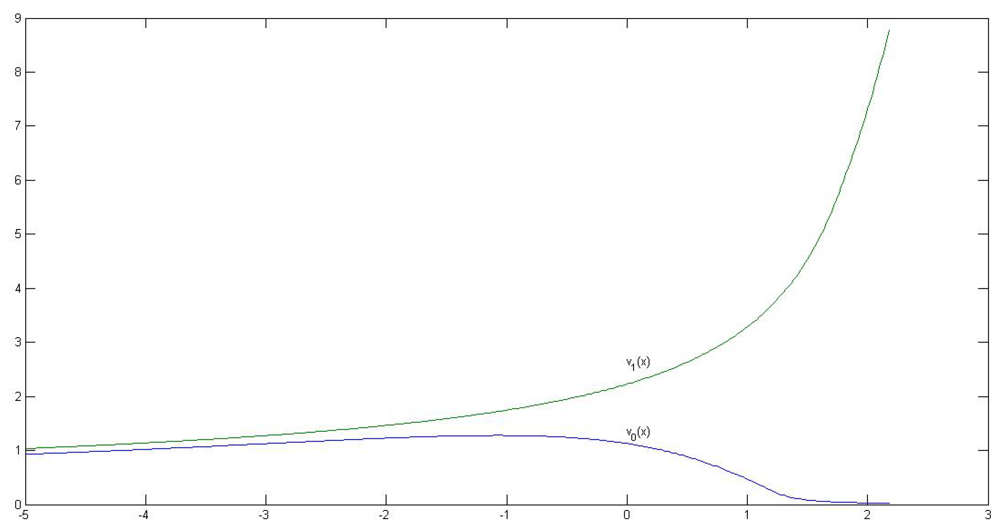
The corresponding value functions $V_0\left(x\right)$ and $V_1\left(x\right)$ are given in Figure 3. Clearly, $V_0\left(x\right)$ is uniformly bounded and $V_1\left(x\right)$ has an exponential growth rate which is consistent to Lemma 1.

We next examine the dependence of $(x_0,x_1,x_2)$. by varying one of the parameters at a time.

In

Table 1. $(x_0,x_1,x_2)$ with varying b.

b	1	1.5	2	2.5	3
$x_0$	−4.36	−4.46	−4.58	−4.66	−4.74
$x_1$	0	0.64	1.22	1.78	2.34
$x_2$	0.74	1.22	1.7	2.18	2.66

, we compute the triple $(x_0,x_1,x_2)$ associated with varying b. Intuitively, a larger b would result larger threshold levels $x_1$ and $x_2$. It can be seen from Table 1 that $x_1$ and $x_2$ are both monotonically increasing as b increases.

In

Table 2. $(x_0,x_1,x_2)$ with varying a.

a	0.6	0.7	0.8	0.9	1
$x_0$	−4.2	−4.4	−4.58	−4.72	−4.86
$x_1$	0.98	1.14	1.22	1.3	1.36
$x_2$	1.58	1.62	1.7	1.74	1.78

, we vary a. Intuitively, a larger a implies larger pulling rate back to the equilibrium level $b=2$, which would encourage more transactions. It can be seen in Table 2 that the lower buying level $x_0$ decreases and the higher buying level $x_1$ increases. This leads to a wider buying interval $[x_0,x_1]$, resulting in greater buying opportunities. The selling level $x_2$ increases but the the interval $[x_1,x_2]$ gets narrower, which suggests one should take profit sooner as a gets bigger.

In

Table 3. $(x_0,x_1,x_2)$ with varying $\sigma$.

$\mathit{\sigma }$	0.3	0.4	0.5	0.6	0.7
$x_0$	−4.56	−4.56	−4.58	−4.58	−4.6
$x_1$	1.12	1.16	1.22	1.28	1.36
$x_2$	1.54	1.62	1.7	1.8	1.9

, we vary the volatility $\sigma$. Intuitively, larger $\sigma$ implies greater range for the stock price $S_t=exp\left(X_t\right)$, which results in higher profit associated with each buying and selling transaction. Table 3 shows that $x_0$ stays flat, and the intervals $[x_0,x_2]$ and $[x_1,x_2]$ both get wider as $\sigma$ increases, which indicates higher profit.

In

Table 4. $(x_0,x_1,x_2)$ with varying $\rho$.

$\mathit{\rho }$	0.3	0.4	0.5	0.6	0.7
$x_0$	−5	−4.86	−4.58	−4.32	−4.12
$x_1$	1.56	1.36	1.22	1.06	0.9
$x_2$	1.94	1.84	1.7	1.56	1.42

, we vary the discount rate $\rho$. Intuitively, larger $\rho$ implies smaller in the value or reward functions, which would discourage transactions. Table 4 shows that $x_0$ increases and the interval $[x_1,x_2]$ gets wider as $\rho$ increases. This indicates one would wait longer to buy or hold the stock longer.

In

Table 5. $(x_0,x_1,x_2)$ with varying K.

K	0.01	0.05	0.1	0.5	1
$x_0$	−5	−5	−4.58	−2.56	−1.6
$x_1$	1.46	1.3	1.22	0.7	−0.46
$x_2$	1.56	1.68	1.7	1.78	1.86

, we vary the transaction cost K. Intuitively, larger K would discourage transactions. Table 5 suggests a similar phenomenon to the case of $\rho$.

Remark 5.

The result in this paper can be used as a guide when implementing a mean-reversion trading. One idea is to start with the trading strategy determined by a parameter triple $(x_0,x_1,x_2)$ and then develop a computational process to estimate these parameters. For example, in (Song et al. 2009), a stochastic approximation method was used to estimate these key levels. The SA algorithm is simple and direct and can be carried out without even assuming the mean reversing dynamics nor worrying about the trouble of model calibration.

4. Conclusions

In this paper, a mean-reverting trading was considered and an optimal rule was given in terms of the triple $(x_0,x_1,x_2)$ corresponding to lows (two buying points) and a high (one selling point). These key levels can be determined by solving a set of quasi-algebraic equations. Moreover, the dependence of the threshold levels $(x_0,x_1,x_2)$ on the parameters is demonstrated in a numerical example.

It would be interesting to consider more realistic models in which the equilibrium levels are subject to jumps. In this case, one may introduce a finite state Markov chain to capture possible jumps. Additional features can be considered include multiple asset trading. Naturally, this will increase the dimension of the problem because one needs to introduce additional decision variables to capture not only when to buy but also which asset to buy over time. It would be interesting to extend the results of this paper to incorporate these practical considerations.

References

- Baccarin, Stefano, and Daniele Marazzina. 2014. Optimal impulse control of a portfolio with a fixed transaction cost. Central European Journal of Operations Research 22: 355–72. [Google Scholar] [CrossRef]
- Baccarin, Stefano, and Daniele Marazzina. 2016. Passive portfolio management over a finite horizon with a target liquidation value under transaction costs and solvency constraints. IMA Journal of Management Mathematics 27: 471–504. [Google Scholar] [CrossRef]
- Blanco, Carlos, and David Soronow. 2001. Mean reverting process—Energy price processes used for derivatives pricing and risk management. Commodities Now, 68–72. [Google Scholar]
- Cowles, Alfred, and Herbert E. Jones. 1937. Some a posteriori probabilities in stock market action. Econometrica 5: 280–94. [Google Scholar] [CrossRef]
- Dai, Min, Qing Zhang, and Qiji Zhu. 2010. Trend following trading under a regime switching model. SIAM Journal on Financial Mathematics 1: 780–810. [Google Scholar] [CrossRef]
- Eloe, Paul, Ruihua Liu, M. Yatsuki, George Yin, and Qing Zhang. 2008. Optimal selling rules in a regime-switching exponential gaussian diffusion model. SIAM Journal on Applied Mathematics 69: 810–29. [Google Scholar] [CrossRef]
- Fama, Eugene F., and Kenneth R. French. 1988. Permanent and temporary components of stock prices. Journal of Political Economy 96: 246–73. [Google Scholar] [CrossRef]
- Gallagher, Liam A., and Mark P. Taylor. 2002. Permanent and temporary components of stock prices: Evidence from assessing macroeconomic shocks. Southern Economic Journal 69: 345–62. [Google Scholar] [CrossRef]
- Guo, Xin, and Qing Zhang. 2005. Optimal selling rules in a regime switching model. IEEE Transactions on Automatic Control 50: 1450–55. [Google Scholar] [CrossRef]
- Hafner, Christian M., and Helmut Herwartz. 2001. Option pricing under linear autoregressive dynamics, heteroskedasticity, and conditional leptokurtosis. Journal of Empirical Finance 8: 1–34. [Google Scholar] [CrossRef] [Green Version]
- Hull, John. 2003. Options, Futures & Other Derivatives. Prentice Hall Finance Series: Options, Futures. Derivatives; Upper Saddle River: Prentice Hall. [Google Scholar]
- Iwarere, Sesan, and B. Ross Barmish. 2010. A confidence interval triggering method for stock trading via feedback control. Paper presented at 2010 American Control Conference, Baltimore, MD, USA, June 30–July 2; pp. 6910–16. [Google Scholar] [CrossRef]
- Leung, Tim, Xin Li, and Zheng Wang. 2015. Optimal multiple trading times under the exponential ou model with transaction costs. Stochastic Models 31: 554–87. [Google Scholar] [CrossRef]
- Løkka, Arne, and Mihail Zervos. 2013. Long-term optimal real investment strategies in the presence of adjustment costs. SIAM Journal Control and Optimization 51: 996–1034. [Google Scholar] [CrossRef]
- Luu, Phong. 2016. Optimal Pairs Trading Rules and Numerical Methods. Ph.D. dissertation, University of Georgia, Athens, GA, USA. [Google Scholar]
- Merhi, Amal, and Zervos Zervos. 2007. A model for reversible investment capacity expansion. SIAM Journal on Control and Optimization 46: 839–76. [Google Scholar] [CrossRef]
- Øksendal, Bernt. 2003. Stochastic Differential Equations: An Introduction with Applications. New York: Springer. [Google Scholar]
- Øksendal, Bernt, and Agnès Sulem. 2002. Optimal consumption and portfolio with both fixed and proportional transaction costs. SIAM Journal on Control and Optimization 40: 1765–90. [Google Scholar] [CrossRef]
- Song, Qingshuo, George Yin, and Qing Zhang. 2009. Stochastic optimization methods for buying-low-and-selling-high strategies. Stochastic Analysis and Applications 27: 523–42. [Google Scholar] [CrossRef]
- Vasicek, Oldrich. 1977. An equilibrium characterization of the term structure. Journal of Financial Economics 5: 177–88. [Google Scholar] [CrossRef]
- Xia, Jianmin, and Xunyu Zhou. 2007. Stock loans. Mathematical Finance 17: 307–17. [Google Scholar] [CrossRef]
- Zhang, Hanqin, and Qing Zhang. 2008. Trading a mean-reverting asset: Buy low and sell high. Automatica 44: 1511–18. [Google Scholar] [CrossRef]
- Zhang, Qing. 2001. Stock trading: An optimal selling rule. SIAM Journal on Control and Optimization 40: 64–87. [Google Scholar] [CrossRef]
- Zhang, Qing, and Xunyu Zhou. 2009. Valuation of stock loans with regime switching. SIAM Journal on Control and Optimization 48: 1229–50. [Google Scholar] [CrossRef]
Figure 1.
Sample paths of and .
Figure 2.
Continuation regions (darkened intervals).
Figure 3.
The value functions and .