Abstract
The chain ladder method is a popular technique to estimate the future reserves needed to handle claims that are not fully settled. Since the predictions of the aggregate portfolio (consisting of different subportfolios) do not need to be equal to the sum of the predictions of the subportfolios, a general multivariate chain ladder (GMCL) method has already been proposed. However, the GMCL method is based on the seemingly unrelated regression (SUR) technique which makes it very sensitive to outliers. To address this issue, we propose a robust alternative that estimates the SUR parameters in a more outlier resistant way. With the robust methodology it is possible to automatically flag the claims with a significantly large influence on the reserve estimates. We introduce a simulation design to generate artificial multivariate run-off triangles based on the GMCL model and illustrate the importance of taking into account contemporaneous correlations and structural connections between the run-off triangles. By adding contamination to these artificial datasets, the sensitivity of the traditional GMCL method and the good performance of the robust GMCL method is shown. From the analysis of a portfolio from practice it is clear that the robust GMCL method can provide better insight in the structure of the data.
1. Introduction
Stochastic claims reserving in non-life insurance, also known as general insurance in the UK or property and casualty insurance in the US, is an important and challenging discipline for actuaries. Since the claims settlement in non-life insurance may last several years, insurers have to set aside money that enables them to handle the liabilities related to current insurance contracts. These outstanding claims reserves are often the largest position on the liability side of the balance sheet of a non-life insurance company.
A well-known and widely used technique to forecast future claims is the chain ladder method, a deterministic algorithm which estimates the future claims recursively using a set of development factors. To include a stochastic component, this simple technique can be embedded into the statistical framework of generalized linear models (GLM), introduced by Nelder and Wedderburn (1972). The relationship between the deterministic chain ladder method and various stochastic models based on GLMs is discussed in England and Verrall (2002) and Wüthrich and Merz (2008) for instance.
A non-life insurance company typically divides portfolios into correlated subportfolios, so that certain homogeneity properties on each subportfolio are satisfied. The chain ladder method is then typically applied to the different subpfortfolios, presented in the form of a single run-off triangle. By doing so, the contemporaneous correlations between these various subportfolios are however ignored. It is well known that the chain ladder predictions for the aggregate portfolio, which consists of the sum of the different subportfolios, is in general different from the sum of the chain ladder predictions for each of the separate subportfolios (Ajne 1994). To address this issue the claims reserving problem is also studied in a multivariate context to cope with the problem of dependence between different subportfolios. Braun (2004) studied the bivariate model which takes into account the correlation between two subportfolios of an aggregate portfolio. Merz and Wüthrich (2007) consider claims reserving for a portfolio consisting of N correlated run-off triangles. Pröhl and Schmidt (2005) and Schmidt (2006) proposed a multivariate chain ladder (MCL) model where they deduced multivariate chain ladder predictors that take into account the dependency between the different subportfolios. These predictors are shown to satisfy a classical optimality criterion. Moreover, it is explained how multivariate methods solve the lack of additivity of the chain ladder predictions. Multivariate methods also have the advantage that we can learn something about the behavior of several subportfolios by observing another subportfolio. Merz and Wüthrich (2008) further discussed the conditional mean squared error of prediction (MSEP) for the MCL model.
Recently, Zhang (2010) proposed a general multivariate chain ladder (GMCL) model that further extends the MCL model by including intercepts to improve model adequacy. The parameters of this flexible model are estimated using the seemingly unrelated regression (SUR) framework. The SUR model (Zellner 1962) is a generalization of a linear regression model which consists of more than one equation and where the error terms of these equations are contemporaneously correlated. The SUR model is very popular and has found many applications in finance and insurance. Taking into account the contemporaneous correlations among different portfolios may lead to more accurate uncertainty assessments. Another advantage is that also structural relationships between triangles where the development of one triangle depends on past losses from other triangles can be included in the GMCL model. The GMCL model also allows joint development of the paid and incurred losses from multiple business lines. The similarity and difference between the GMCL model on bivariate data and the Munich chain ladder model (Quarg and Mack 2004) are discussed by Zhang (2010), who also shows that several existing multivariate claims reserving estimators can find their equivalent in the SUR estimator family.
To estimate the parameters in a SUR model, one typically uses the feasible generalized least squares (FGLS) estimator (Zellner 1962), which takes into account the covariance structure of the errors. Since FGLS is based on the classical covariance matrix and ordinary least squares estimation, using FGLS makes the SUR estimates and thus in particular the GMCL estimates very sensitive to outliers, which are data points that deviate from the pattern suggested by the majority of the data. Such atypical observations may have a large impact on traditional statistical techniques. On the other hand, robust statistics aim to obtain estimates for the claim provisions that is close to the classical estimates applied on the data without the outliers (without modeling the outlier generating process). As a consequence of fitting the majority of the data well, the outliers can be reliably detected by their large deviations from this fit. The flagged outliers may then be inspected by experts. In Koenker and Portnoy (1990) a robust SUR estimator is proposed based on M-estimators. Since this procedure is not affine equivariant and does not take full account of the multivariate nature of the problem, a method based on S-estimators was introduced in Bilodeau and Duchesne (2000). This robust SUR estimator is regression and affine equivariant, but is computationally expensive. Therefore, Hubert et al. (2017) proposed the FastSUR algorithm, which implements the ideas of the FastS algorithm (Salibian-Barrera and Yohai 2006) for the SUR S-estimator. Recently, Peremans and Van Aelst (2018) developed robust inference for the SUR model based on MM-estimators.
This paper is structured as follows. A review of the GMCL model of Zhang (2010) is given in Section 2. In Section 3 the GMCL model is formulated in the SUR framework and the FGLS estimator is introduced. Section 4 describes robust MM-estimators for estimating the parameters in GMCL models and its numerical algorithm for computation. We then show the good performance of these estimators in an extensive simulation study in Section 5. In Section 6 the robust procedure is illustrated on a real dataset from a non-life business line. Some concluding remarks and potential directions for further research are given in Section 7. The Appendix contains the parameter estimates obtained from the GMCL models for the real dataset.
2. General Multivariate Chain Ladder Model
We assume that the non-life insurance company needs to handle subportfolios. Let I and K denote the final accident and development period respectively. For , and denote the random variable as the cumulative claims amount of accident period i and development period k of subportfolio m. Depending on the size of K, one refers to long or short tail business and for simplicity we take .
At time I the claims with are observed, while the claims with are not observed. Typically, the observed claims of subportfolio m are then presented in the structure of a run-off triangle as illustrated in Table 1.

Table 1.
Typical representation of subportfolio m as a run-off triangle.
This triangle structure shows the development of claims for each accident period. Usually yearly, quarterly or monthly periods are used. The columns represent the development periods whereas the diagonals present payments in the same calendar period. The overall outstanding reserve R that will need to be paid in future, is defined as
and depends on the ultimate claim values . The aim of claims reserving is then to complete the run-off triangles into squares, i.e., forecasting the future claims in the bottom right corner of the run-off triangles in order to estimate the overall outstanding reserves.
Let denote the vector of cumulative claims of accident period i and development period k. Consider the following model structure from development period k to :
where is the M vector containing intercepts , is the matrix that contains the development parameters for run-off triangle m in row m, and are independent (over i) and symmetrically distributed random vectors representing the error terms. For a non-diagonal development matrix , the model allows the development of one run-off triangle in development period k to depend linearly on the claims in the other run-off triangles at development period k. Moreover, it is assumed that the errors satisfy
where is the set of cumulative claims for accident period i up to and including development period k, is a symmetric positive definite matrix, and is the operator that turns its argument(s) into a diagonal matrix. Consequently, for a non-diagonal matrix the components of the error terms are allowed to be correlated. Equations (1)–(3) for development periods constitute the general multivariate chain ladder (GMCL) model as proposed in Zhang (2010). Hence, the GMCL model is a collection of linear models. A separate chain ladder (SCL) model can be obtained as a special case by taking the zero vector, and by imposing that and are diagonal matrices. The advantages of the GMCL model over already existing models like SCL are evident (Zhang 2010). The parameters , and are unknown model parameters and need to be estimated from historic claims in order to predict future losses.
4. Robust GMCL Method
In the univariate setting () Verdonck and Debruyne (2011) have demonstrated that outliers can affect the chain ladder method so strongly that there is huge over- or underestimation of the overall reserve estimate. Several robust alternatives have already been developed in the univariate claims reserving framework (see e.g., Brazauskas et al. (2009); Brazauskas (2009); Verdonck et al. (2009); Verdonck and Van Wouwe (2011); Pitselis et al. (2015); Peremans et al. (2017)). Hubert et al. (2017) have shown that FGLS estimators in the GMCL model are also very sensitive to outliers. Please note that the multivariate aspect makes the task of outlier detection more challenging because outliers can be univariate or multivariate. Multivariate outliers are observations that deviate from the multivariate pattern indicated by the majority of the observations, i.e., inconsistent with the covariance structure of the dataset, but in contrast to univariate outliers are not necessarily extreme along a single coordinate (a single run-off triangle). Therefore, univariate outlier detection methods may fail to find these outliers and it is important to rely on robust multivariate alternatives. We propose a robust methodology for reserve estimates and outlier detection by combining robust SUR estimators with the GMCL model.
We now introduce MM-estimators for the SUR model in (5) as studied by Peremans and Van Aelst (2018). The system of equations in (5) can be rewritten as another linear regression model by reordering the equations. Let , and be the subvector or submatrix of , and respectively by extracting rows . Then the system of equations in (5) is equivalent to
In this case we easily obtain that . Decompose the covariance matrix into a shape component and a scale parameter such that with . Here denotes the determinant of the matrix . Since we assume that is positive definite, such a decomposition always exists. Let be equal to for any vector according to the SUR representation in (8). Then, given an initial estimator of the scale , the MM-estimators minimize
over all vectors and positive definite symmetric matrices with . The MM-estimator for covariance is defined as . Evidently, taking yields the iterated FGLS estimator. To be robust against outliers, it is necessary to consider bounded functions. More specifically, we assume that the function satisfies the following conditions:
- is symmetric, twice continuously differentiable and satisfies ;
- is strictly increasing on and constant on for some .
The most favored family of functions for MM-estimators is the class of Tukey bisquare functions given by . The tuning parameter is usually chosen to obtain a certain level of asymptotic efficiency under the SUR model with normally distributed errors. From now on, we will always consider Tukey bisquare function with tuning parameter (to obtain MM-estimators with efficiency under the normal model).
MM-estimators require an initial estimator of scale . In order for MM-estimators to be robust, also this scale estimator should be robust. Therefore, highly robust S-estimators are computed to obtain a highly robust scale estimator. S-estimators have been introduced for SUR models in Bilodeau and Duchesne (2000), and a computational efficient algorithm has been proposed in Hubert et al. (2017). Robustness can be measured by the breakdown point of an estimator, which is roughly equal to the maximal fraction of contaminated observations that an estimator can tolerate before its bias becomes unbounded. For MM-estimators the breakdown point can be up to . In this paper we have tuned the MM-estimators to have a 25% breakdown point and 95% normal efficiency, which is commonly considered to be a good compromise between robustness and precision of the estimator.
MM-estimators do not have explicit solutions, although they satisfy a similar set of equations as the FGLS estimators given in (7). Indeed, the MM-estimators satisfy the following set of equations
with where , , and are the residuals derived from the representation in (8). Starting from the initial S-estimates, MM-estimates are computed simply by iterating these estimating equations until convergence. If w is bounded and non-increasing, the convergence of this iterative procedure to a local minimum is guaranteed (Maronna et al. 2006). The function w can be interpreted as a weight function that can be used to identify outliers. Indeed, a small value of corresponds with a large residual distance and indicates that the observation corresponding to accident period i is an outlier. For more details on the properties of S and MM-estimators, we refer to Peremans and Van Aelst (2018). We now explore the use of these robust estimators in the GMCL model to obtain robust reserve estimates and identify outliers in the run-off triangles.
5. Simulation Study
First, we introduce a simulation design according to the GMCL model to generate multivariate run-off triangles. Then, we investigate the prediction performance of the classical and robust estimators for GMCL models by simulation.
We consider the case where two run-off triangles are available (), but the results can easily be generalized to more triangles (). To generate two run-off triangles under the GMCL model in (1), we first generate for and independently from a uniform distribution on the interval . These numbers represent the losses observed in the first development period. Then, let
for with . The entries of the first (second) rows determine the increase of the cumulative claims of the first (second) triangle. Please note that the structural connections among triangles, i.e., the non-diagonal entries of , decrease towards zero for to ensure that the cumulative claims stabilize at a certain point in time. Furthermore, assume that the error terms from the representation in (8) are independently and normally distributed with mean zero and covariance . The covariance matrices are defined by multiplying the equicorrelation matrix with correlation 0.5 by the scalar for . This choice of leads to error terms that become smaller for . If no shrinkage would be applied on the covariance matrices, then the error terms would grow on average because they are linearly related to the cumulative claims of the previous period which increase over time. Finally, the cumulative claims for , and can be computed according to the GMCL model in (1) by generating independent error terms from the aforementioned error distribution. We have chosen the parameters , and such that the resulting run-off triangles resemble real data. The cumulative and incremental claims of two run-off triangles simulated according to this data generating process are shown in Figure 1.
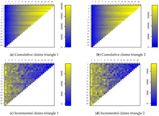
Figure 1.
Cumulative and incremental claims for a pair of dependent run-off triangles. Development periods are on the horizontal axis, accident periods are on the vertical axis. The bar plot represents a color code indicating the magnitude of the numbers.
Please note that the patterns in these run-off triangles behave similar for every accident period.
Consider the prediction of a single cell of subportfolio m for , i.e., the prediction of a future loss. Given historic claims of M subportfolios, the development parameters and of the GMCL model can be estimated for . Following the GMCL model these parameter estimators yield a corresponding prediction estimator for . To measure the prediction accuracy of the estimator , we consider its mean squared error of prediction (MSEP), given by
Since in general it is not possible to derive a simple expression for the MSEP, we adopt a Monte-Carlo simulation strategy to estimate this quantity. By repeatedly generating M run-off triangles as described before, fitting the GMCL model and predicting through the computation of the estimator , we obtain J prediction estimators denoted by . Then, an estimator of the MSEP of is given by
Smaller values of MSEP indicate a better prediction performance. In our simulation results we will report the square root of the MSEP denoted by RMSEP.
For data simulated as described before we consider three procedures: the SCL model in combination with LS (in short SCL-LS) and the GMCL model in combination with FGLS and robust MM-estimators (in short GMCL-FGLS and GMCL-MM respectively). As noted by Zhang (2010, pp. 595–96) it is difficult to fit the SUR models for the upper right part of the triangles because the data is scarce. To avoid numerical instabilities, it is recommended to use SCL for the development in the tail. Naturally, we advice to combine the robust procedure based on MM-estimators with a robust SCL method such as proposed in Verdonck and Debruyne (2011) for the tail development. Since the focus of this paper is on the multivariate model, we present all results without the tail development part, i.e., the final 10 development periods using traditional or robust SCL.
Consider the prediction of the expected claim size for . The top right panel of Figure 2 shows the estimated RMSEP of for SCL-LS, GMCL-FGLS and GMCL-MM as a function of the total number of accident periods I ranging from 25 to 50 for simulations.
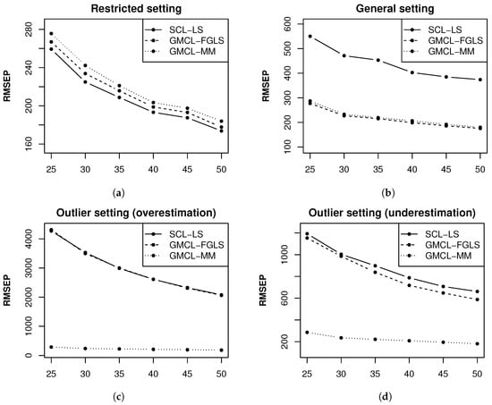
Figure 2.
RMSEP estimates of obtained from SCL-LS, GMCL-FGLS and GMCL-MM as a function of I for the restricted, general and outlier settings.
We can see that the RMSEP estimates are larger for SCL-LS. This is expected because SCL does not take structural connections among run-off triangles into account and contemporaneous correlations between the error terms of the run-off triangles are ignored. Please note that GMCL-FGLS and GMCL-MM perform similarly in this setting where the triangles contain only regular measurements. Moreover, similar performance was obtained for and hence, these results are omitted.
We now change the parameters , and in the simulation design in such a way that it matches the SCL structure. For take
and let be the identity matrix multiplied with the scalar . In this setting SCL is optimal, whereas the GMCL model uses too many parameters. Intercepts, slopes measuring the effects of the other triangles and correlation parameters are unnecessary in this case. When we compare the results of both estimation procedures, presented in the top left window of Figure 2, we observe that the RMSEP is only slightly larger for GMCL models.
To illustrate the sensitivity of the classical procedures and the robustness of MM-estimators, we now consider the following outlier setting: for each pair of run-off triangles we replace the simulated error term to generate with . Based on generated pairs of triangles of this kind, we obtained the results in the bottom left panel of Figure 2. Clearly, both classical estimates break down because they largely overestimate , while the robust estimates are not influenced by the outliers. The robust results are similar to the classical results that were obtained when no outliers were present in the data. We also show the effect of small losses in run-off triangles. Therefore, we consider a second outlier setting: for each pair of run-off triangles we replace with . The bottom right plot of Figure 2 shows the RMSEP estimates for this outlier setting. Now, both classical estimators underestimate due to a small loss observed in accident period two, leading to large RMSEP values. On the other hand, the robust method resists the effect of the outlier and still performs well. In both outlier settings the robust method can also detect the outlier because the weight of the corresponding accident period is zero as can be seen in Figure 3 for the first outlier setting.
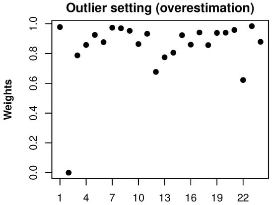
Figure 3.
Weights obtained from GMCL-MM for a pair of dependent run-off triangles with one outlier.
For the second outlier setting the plot of weights is nearly identical.
To illustrate the impact of the outlier’s distance to the regular data, we also consider a third outlier setting: for each pair of run-off triangles we replace the simulated error term to generate with where d ranges from −1 to 1. Non-contaminated error terms take values between −3000 and 3000 for the first development period. Therefore, the situations when are cases with outliers. Again bivariate run-off triangles are generated and the prediction accuracy of the expected claim is measured by MSEP. As opposed to the previous simulations we now fix the number of accident periods I to 25. Figure 4 contains the RMSEP results for different outlier distances d.
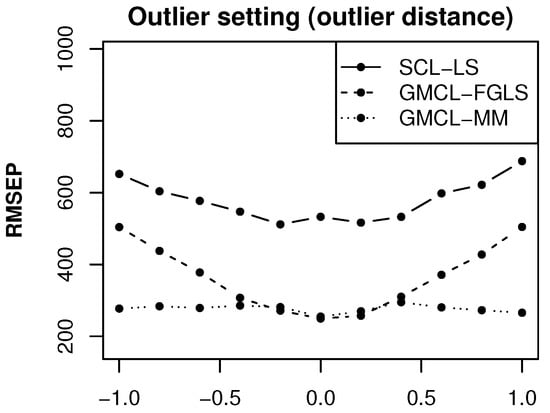
Figure 4.
RMSEP estimates of obtained from SCL-LS, GMCL-FGLS and GMCL-MM as a function of the outlier distance d.
When no outliers are generated and the prediction performance of the procedures GMCL-FGLS and GMCL-MM are identical, as we have seen before. For situations with outliers the classical methods yield large RMSEP values because their predictions under- or overestimate the target claim due to the presence of the outliers. The larger the outlier distance d, the worse the prediction accuracy is for non-robust methods. On the other hand, the prediction estimates obtained from the robust method remain stable for all situations.
A more general case is to consider the prediction of for with . In particular, we consider . We repeat the same procedure of squaring pairs of dependent triangles and measure the prediction accuracy of by means of RMSEP. The results for the general setting are shown in Figure 5. The performance of the different methods is comparable to their performance in the previous setting when predicting . However, since the prediction of depends on 14 model fits, and consequently, the MSEP estimates of become much larger. The prediction performance in the restricted setting and outlier settings (not shown) are also similar as before.
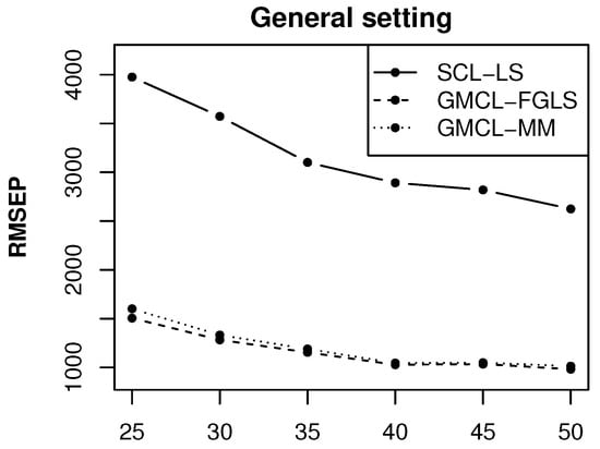
Figure 5.
RMSEP estimates of obtained from SCL-LS, GMCL-FGLS and GMCL-MM as a function of I for the general setting.
We have also investigated how the position of the outlier influences the prediction performance. Here the outlier’s position refers to the development period in which it has occurred because the effect is similar for all accident years. If the outlier occurs after the target claim, then both the classical and robust methods yield reliable prediction results for the target claim. However, when the outlier occurs before the target claim, then the classical methods yield prediction estimates that are affected by the outlier, while the robust method remains reliable. Only when the outlier appears in the upper right tail of a run-off triangle, it will affect any method, whether it is robust or not, because there is not enough data available in this tail to be able to identify an outlier. Since the position of outliers is unknown in practice, this illustrates the importance of robust procedures which offer protection against outliers in almost any position of the run-off triangles.
6. Real Data
To illustrate the new methodology, we consider an example with paid and incurred data from a motor third party liability (MTPL) and a general third party liability (GTPL) insurance portfolio from a non-life insurance company operating in Belgium. The data have been recorded between March 2008 and December 2015. Quarterly data are available leading to run-off triangles of dimension shown in Figure 6.
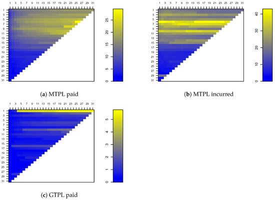
Figure 6.
Cumulative run-off triangles (divided by 100,000) of a real insurance portfolio. Development periods are on the horizontal axis, accident periods are on the vertical axis. The bar plot represents a color code indicating the magnitude of the numbers.
Observe that from accident trimester 15 onwards the cumulative claim amounts for MTPL become much smaller. This effect is due to a decrease in total premium volume, and hence, also in total number of claims. For the GTPL data, accident trimester 1 seems suspicious. The claim amounts are much larger in comparison to any other period. Finally, notice that for the first 15 accident trimesters the losses in the subportfolios are almost fully developed, i.e., the changes in consecutive cumulative claims are minuscule in the last development years.
We model these run-off triangles separately with SCL and jointly with GMCL. The joint model is given by Equation (1) with . The separate model simplifies the joint model by excluding intercepts, structural connections and contemporaneous correlations. We have applied SCL-LS, GMCL-FGLS and GMCL-MM to square the run-off triangles up until period 21. As explained before, we exclude the tail development part in order to focus on the multivariate models.
Table A1 in Appendix A contains the estimates of the development parameters and the sample correlations between the resulting residuals obtained by SCL-LS for all development periods. While the run-off triangles have been modeled separately, for some development periods there are substantial correlations between the residuals which indicates that the independence assumption might be violated for these data.
The parameter estimates obtained from GMCL-FGLS are summarized in Table A2 in Appendix A. The slope estimates and measure the contribution of the other two triangles when predicting future losses in a triangle. From Table A2 it can be seen that for some development periods these estimates are substantially different from zero. They improve the model fit and the prediction performance. The last three columns of Table A2 contain the sample correlations between the residuals of the three run-off triangles, which have been obtained as
for , where are the entries of the covariance matrix . Several moderate to large correlations have been obtained which again supports the joint GMCL model for these data.
We now apply the robust method GMCL-MM which yields the development parameter estimates shown in Table A3 in Appendix A. Based on this robust procedure we can now detect possible outliers. The weights assigned to each observation in the SUR models are shown in Figure 7.
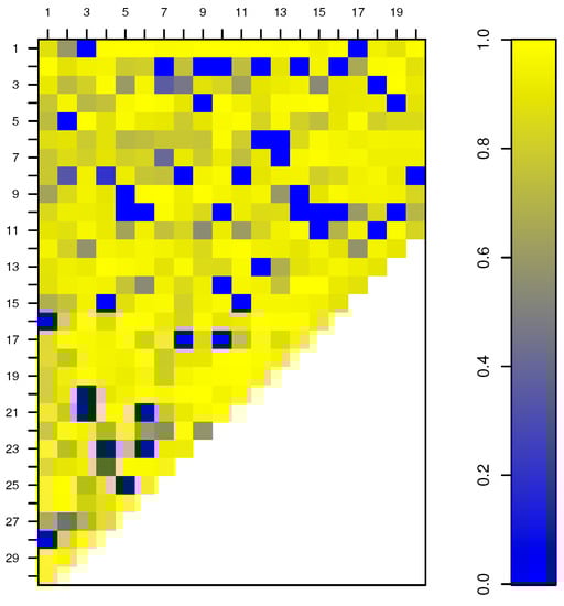
Figure 7.
Weights obtained from GMCL-MM for a real insurance portfolio. Each row corresponds to an accident trimester used in the fitting procedure. Each columns represents a SUR model.
The smaller the weight, the more outlying is an observation with respect to the bulk of the data. For example, from Figure 7 we can observe that in the first development period there are two major outliers corresponding to accident trimesters 16 and 28 respectively.
The outliers identified by the GMCL-MM method may have affected the classical estimators, and hence, also the prediction of future losses. Hence, in Table 2 we compare the total reserve estimates for all methods.
Table 2.
Total reserve estimates for all run-off triangles of a real insurance portfolio obtained from SCL-LS, GMCL-FGLS and GMCL-MM.
Let us first focus on the paid losses of the MTPL portfolio. The non-robust SCL-LS and GMCL-FGLS methods both yield a total reserve estimate that is larger than for the robust GMCL-MM. A close inspection of the predicted run-off triangles revealed that the transition from development trimester 20 to 21 is highly responsible for these large differences. For development trimester 21 one can observe in Figure 6 a large incremental increase of the losses that occurred in accident trimester 8. The SCL-LS and GMCL-FGLS fits for this transition period are both largely influenced by this particular observation. Consequently, the predicted future losses from this development trimester onward are much larger. On the other hand, the robust GMCL-MM method is much less influenced by this observation and is able to flag this observation as an outlier.
Let us now consider the reserve estimates of the incurred losses. The two non-robust approaches agree quite well. The difference is mainly caused by accident trimester 29 for which unexpectedly small paid losses have been observed but at the same time large incurred losses were recorded. In the joint GMCL model the development factor for the model from development period 7 to 8 differs from zero and thus influences the incurred losses obtained by GMCL-FGLS which is not the case for SCL-LS. Moreover, remark that these reserve estimates are negative. Negative reserve estimates are often observed for incurred run-off triangles due to overestimation of the losses. The robust total reserve estimate obtained by GMCL-MM is much larger than for the non-robust methods. This indicates that the presence of outliers has again affected the classical results. More specifically, in this case the classical procedures yield smaller prediction estimates as compared to the robust procedure. For example, one can verify that for the transition from development trimester 18 to 19 the prediction estimates obtained by GMCL-MM are much larger than those obtained by GMCL-FGLS.
Finally, we also consider the estimated reserve for the GTPL portfolio. The unusual data in the first accident trimester affect the total reserve estimates of both non-robust methods. On the other hand, the robust GMCL-MM detected the deviating pattern in the first accident trimester as well as other moderate outliers and yields a robust total reserve estimate that is not driven by atypical behavior in the available data. Please note that the GMCL-based methods yield negative reserve estimates for these data. While negative reserve estimates are not uncommon for incurred losses, they are rather unusual for run-off triangles with paid losses. However, the real data have been obtained from a small company and the company informed us that for some claims there has been substantial recovery of initially paid losses. These recoveries have an impact on the cumulative claims data which may explain the negative reserve estimates in this case.
To further investigate the performance of the estimation methods, we now focus on the prediction of the values on the last diagonal of all run-off triangles. To measure the accuracy of the predictions, we consider their MSEP. More specifically, we leave out the last diagonal of all three run-off triangles, apply the different methods on the remaining data and calculate the mean squared relative prediction error for each method. The results are given in Table 3 for each subportfolio separately as well as all portfolios jointly.
Table 3.
MSEP for the last diagonal of all run-off triangles (and totals) of a real insurance portfolio obtained from SCL-LS, GMCL-FGLS and GMCL-MM.
While the three methods perform quite similar on the first two run-off triangles, this is not the case for the GTPL paid data as can be seen from Table 3. The MSEP of GMCL-FGLS is large for this run-off triangle. SCL-LS performs better, but not as good as GMCL-MM which is the only method that yields reasonable performance for these data. As a result, GMCL-MM also shows the best overall performance which illustrates that the outliers in these run-off triangles affect the predictions of the non-robust methods.
7. Conclusions
In this paper, we have presented a robust estimation method for the general multivariate chain ladder model proposed by Zhang (2010). Hence, our proposed methodology takes into account contemporaneous correlations and structural connections between different run-off triangles and still yields reliable results when the data are contaminated. Moreover, it allows us to automatically identify the most influential and atypical claims in the run-off triangles.
We believe that experts should then further examine these flagged outliers to find out why these observations are atypical. If the outlier(s) are simply errors or are very unlikely to happen again in future, then the robust results can be used as reserve estimates. However, if it is likely that similar outliers will re-occur in future, then we advice to model their process so that one can predict how much money will be needed for these deviations in future years. The final total reserve estimate may then be equal to the robust total reserve estimate and a safe margin based on this prediction. Note that it can also happen that outliers lead to an underestimation of the total reserve estimate even if the atypical claims are larger than the expected claims.
The robust GMCL method was applied to simulated run-off triangles illustrating its excellent performance. From a portfolio analysis of real run-off triangles from a small non-life insurance company in Belgium it was clear that the proposed robust methodology is helpful to gain insight in the data and to build up a more realistic reserve, certainly when it is used in addition to the classical multivariate chain ladder method.
Author Contributions
The authors contributed equally to this work.
Funding
This research was funded by International Funds KU Leuven grant numbers C16/15/068 and C24/15/001, the CRoNoS COST Action grant number IC1408 and the Flemish Science Foundation (FWO) grant number 1523915N.
Conflicts of Interest
The authors declare no conflict of interest.
Appendix A
Table A1.
Development parameter estimates and empirical correlation estimates obtained from SCL-LS for a real insurance portfolio.
Table A1.
Development parameter estimates and empirical correlation estimates obtained from SCL-LS for a real insurance portfolio.
| k | ||||||
|---|---|---|---|---|---|---|
| 1 | 1.29 | 1.04 | 1.88 | 0.13 | 0.51 | 0.04 |
| 2 | 1.14 | 1.01 | 1.18 | −0.22 | −0.08 | 0.13 |
| 3 | 1.08 | 0.99 | 1.35 | 0.20 | −0.08 | −0.08 |
| 4 | 1.05 | 1.01 | 1.06 | 0.26 | −0.02 | −0.09 |
| 5 | 1.04 | 1.00 | 1.12 | 0.11 | −0.02 | 0.18 |
| 6 | 1.03 | 1.00 | 1.05 | −0.22 | −0.01 | 0.08 |
| 7 | 1.03 | 1.00 | 1.01 | −0.14 | −0.11 | 0.53 |
| 8 | 1.02 | 0.99 | 1.03 | 0.38 | 0.14 | 0.26 |
| 9 | 1.02 | 0.99 | 1.02 | 0.39 | 0.14 | 0.01 |
| 10 | 1.01 | 1.01 | 1.01 | 0.36 | −0.11 | 0.17 |
| 11 | 1.02 | 1.00 | 1.01 | −0.35 | −0.01 | −0.03 |
| 12 | 1.01 | 0.99 | 1.03 | 0.26 | 0.16 | 0.08 |
| 13 | 1.01 | 1.01 | 1.02 | −0.29 | −0.13 | −0.28 |
| 14 | 1.01 | 0.99 | 1.03 | 0.17 | 0.05 | −0.28 |
| 15 | 1.02 | 0.99 | 1.02 | 0.11 | −0.23 | −0.01 |
| 16 | 1.01 | 0.99 | 1.01 | 0.09 | 0.43 | 0.49 |
| 17 | 1.01 | 1.00 | 1.03 | −0.23 | −0.17 | 0.24 |
| 18 | 1.01 | 0.99 | 1.03 | −0.54 | −0.18 | −0.08 |
| 19 | 1.01 | 0.99 | 1.03 | 0.08 | −0.28 | 0.32 |
| 20 | 1.04 | 0.99 | 1.01 | −0.37 | −0.07 | −0.04 |
Table A2.
Development parameter estimates and correlation estimates obtained from GMCL-FGLS for a real insurance portfolio.
Table A2.
Development parameter estimates and correlation estimates obtained from GMCL-FGLS for a real insurance portfolio.
| k | |||||||||||||||
|---|---|---|---|---|---|---|---|---|---|---|---|---|---|---|---|
| 1 | 23,397.72 | 1.14 | 0.02 | 0.93 | −11.47 | 0.08 | 1.00 | 0.83 | 21,694.08 | −0.02 | 0.00 | 1.22 | 0.20 | 0.50 | 0.03 |
| 2 | 15,223.35 | 1.09 | 0.01 | −0.15 | 20,020.27 | 0.12 | 0.95 | −0.23 | 1727.03 | 0.01 | 0.00 | 1.07 | −0.22 | −0.10 | 0.04 |
| 3 | 16,228.14 | 0.99 | 0.04 | −0.14 | 15,116.47 | −0.01 | 0.99 | −0.03 | −12,277.95 | 0.05 | −0.02 | 1.57 | 0.23 | 0.02 | −0.07 |
| 4 | 10,350.14 | 1.00 | 0.03 | −0.06 | 50,876.00 | −0.07 | 1.03 | −0.11 | 4182.92 | 0.00 | 0.00 | 1.00 | 0.23 | −0.19 | −0.23 |
| 5 | 1028.93 | 0.94 | 0.05 | −0.01 | −6957.99 | −0.05 | 1.04 | 0.01 | −1377.61 | 0.02 | −0.01 | 1.01 | −0.01 | 0.04 | 0.19 |
| 6 | 12,243.16 | 0.97 | 0.03 | −0.03 | 8286.35 | 0.06 | 0.98 | −0.36 | 10,968.80 | 0.00 | 0.00 | 0.97 | −0.29 | −0.01 | −0.01 |
| 7 | −3719.21 | 1.02 | 0.00 | 0.04 | −6260.32 | −0.13 | 1.07 | 0.00 | −379.22 | 0.00 | 0.00 | 1.00 | −0.22 | −0.05 | 0.62 |
| 8 | −755.07 | 1.03 | 0.00 | −0.01 | 5287.58 | −0.04 | 1.00 | 0.17 | −1120.14 | 0.00 | 0.00 | 1.01 | 0.41 | 0.19 | 0.45 |
| 9 | −11,302.41 | 1.05 | −0.01 | −0.07 | −4825.36 | 0.00 | 1.00 | −0.08 | 904.91 | 0.00 | 0.00 | 1.00 | 0.36 | 0.08 | −0.05 |
| 10 | 6920.22 | 0.97 | 0.03 | 0.01 | 37,848.84 | −0.15 | 1.09 | −0.06 | 502.78 | 0.00 | 0.00 | 1.00 | 0.17 | −0.02 | 0.24 |
| 11 | 9660.89 | 0.95 | 0.04 | 0.00 | −27,830.17 | 0.09 | 0.96 | −0.05 | −438.20 | 0.00 | 0.00 | 1.02 | −0.26 | 0.20 | −0.04 |
| 12 | −16,214.89 | 1.01 | 0.01 | 0.00 | 8784.70 | −0.07 | 1.03 | 0.10 | −1370.21 | 0.01 | 0.00 | 1.00 | 0.20 | 0.14 | 0.16 |
| 13 | −18,821.47 | 1.00 | 0.02 | 0.01 | −30,184.25 | −0.08 | 1.07 | 0.08 | −1385.69 | 0.01 | 0.00 | 1.00 | −0.44 | 0.02 | −0.16 |
| 14 | −17,224.86 | 1.00 | 0.02 | 0.00 | 40,874.99 | −0.06 | 1.02 | −0.19 | −11,617.13 | 0.01 | 0.00 | 1.02 | 0.08 | 0.08 | −0.32 |
| 15 | −20,373.50 | 1.02 | 0.00 | 0.12 | −24,051.79 | 0.06 | 0.97 | −0.11 | −7141.82 | 0.00 | 0.00 | 1.01 | 0.20 | −0.21 | −0.12 |
| 16 | −2082.74 | 1.02 | 0.00 | −0.02 | 17,582.20 | 0.02 | 0.98 | −0.05 | 1397.56 | 0.00 | 0.00 | 1.00 | 0.05 | 0.36 | 0.43 |
| 17 | −44,523.11 | 1.04 | 0.00 | −0.02 | 61,268.64 | −0.04 | 1.00 | 0.03 | 2554.84 | 0.00 | 0.00 | 1.05 | −0.07 | −0.04 | −0.11 |
| 18 | −13,650.45 | 1.02 | 0.00 | −0.03 | −51,338.15 | 0.02 | 0.99 | 0.05 | −6862.07 | 0.01 | 0.00 | 1.04 | −0.56 | −0.13 | −0.10 |
| 19 | −37,910.90 | 1.01 | 0.01 | 0.06 | 4693.44 | 0.00 | 0.99 | 0.02 | −55,064.83 | 0.04 | 0.00 | 0.97 | 0.06 | −0.45 | 0.56 |
| 20 | 874,470.74 | 0.53 | 0.07 | −0.48 | −76,063.75 | 0.04 | 0.99 | 0.01 | −1304.77 | 0.00 | 0.00 | 1.00 | −0.31 | −0.18 | −0.03 |
Table A3.
Development parameter estimates and correlation estimates obtained from GMCL-MM for a real insurance portfolio.
Table A3.
Development parameter estimates and correlation estimates obtained from GMCL-MM for a real insurance portfolio.
| k | |||||||||||||||
|---|---|---|---|---|---|---|---|---|---|---|---|---|---|---|---|
| 1 | 7820.38 | 1.15 | 0.02 | 1.16 | −3680.41 | 0.08 | 1.00 | 1.03 | 1717.07 | 0.01 | 0.00 | 1.11 | 0.24 | −0.31 | 0.06 |
| 2 | 12,144.56 | 1.09 | 0.01 | −0.11 | 16,619.03 | 0.13 | 0.95 | −0.19 | 873.94 | 0.01 | 0.00 | 1.06 | 0.20 | 0.11 | −0.10 |
| 3 | 23,528.36 | 1.00 | 0.03 | −0.20 | 22,422.99 | 0.00 | 0.98 | −0.10 | 1918.65 | 0.01 | 0.00 | 0.99 | 0.08 | 0.30 | 0.10 |
| 4 | 8438.94 | 1.01 | 0.02 | −0.04 | 891.69 | 0.06 | 0.97 | −0.11 | 4896.14 | 0.00 | 0.00 | 1.00 | 0.03 | 0.00 | 0.21 |
| 5 | −2355.67 | 0.98 | 0.03 | −0.02 | −30,886.96 | −0.06 | 1.05 | 0.04 | 1715.40 | −0.01 | 0.00 | 1.03 | −0.03 | −0.21 | −0.04 |
| 6 | 8351.98 | 0.97 | 0.04 | −0.04 | 9538.34 | 0.07 | 0.97 | −0.33 | −209.96 | 0.00 | 0.00 | 1.00 | −0.29 | −0.20 | −0.08 |
| 7 | −2873.28 | 1.02 | 0.00 | 0.03 | −4771.62 | −0.12 | 1.07 | 0.02 | −243.36 | 0.00 | 0.00 | 1.00 | −0.23 | −0.17 | 0.64 |
| 8 | −806.41 | 1.00 | 0.01 | 0.01 | 821.12 | −0.06 | 1.02 | 0.13 | −1135.19 | 0.00 | 0.00 | 1.01 | 0.06 | 0.09 | 0.32 |
| 9 | −6931.74 | 1.03 | 0.00 | −0.03 | 1925.54 | −0.03 | 1.01 | −0.02 | 1272.45 | 0.00 | 0.00 | 1.00 | −0.19 | 0.21 | 0.02 |
| 10 | 8446.18 | 0.97 | 0.02 | 0.00 | 13,573.18 | 0.00 | 0.99 | −0.06 | 44.18 | 0.00 | 0.00 | 1.00 | −0.46 | −0.05 | −0.17 |
| 11 | −1481.68 | 0.98 | 0.03 | 0.00 | −3558.47 | 0.04 | 0.97 | 0.04 | −588.16 | 0.00 | 0.00 | 1.02 | −0.02 | 0.15 | −0.03 |
| 12 | −19,036.01 | 1.01 | 0.01 | 0.00 | 10,657.18 | −0.07 | 1.03 | 0.08 | −1020.05 | 0.00 | 0.00 | 1.00 | 0.13 | 0.77 | 0.10 |
| 13 | −17,979.52 | 1.03 | 0.00 | −0.02 | 21,175.00 | −0.07 | 1.03 | 0.08 | −1469.87 | 0.01 | 0.00 | 1.00 | 0.23 | −0.25 | −0.18 |
| 14 | −6110.32 | 1.01 | 0.00 | 0.00 | −21,779.08 | 0.02 | 1.00 | −0.08 | −4066.28 | 0.00 | 0.00 | 1.00 | −0.34 | 0.66 | 0.16 |
| 15 | −2628.61 | 0.99 | 0.00 | 0.15 | −20,629.80 | 0.05 | 0.97 | −0.10 | 219.13 | 0.00 | 0.00 | 1.01 | −0.07 | −0.50 | −0.11 |
| 16 | 621.54 | 1.02 | 0.00 | −0.03 | −42,626.20 | 0.03 | 1.00 | −0.05 | −2510.24 | 0.00 | 0.00 | 0.99 | −0.59 | 0.79 | −0.22 |
| 17 | −39,374.59 | 1.04 | 0.00 | −0.10 | 70,972.58 | −0.07 | 1.00 | 0.25 | 2017.96 | 0.00 | 0.00 | 1.00 | 0.15 | −0.12 | 0.60 |
| 18 | 25,424.10 | 0.98 | 0.01 | −0.02 | 101,648.10 | −0.11 | 1.03 | 0.09 | −25,270.86 | 0.02 | −0.01 | 1.02 | 0.12 | 0.09 | −0.97 |
| 19 | −42,462.66 | 1.02 | 0.02 | −0.11 | 74,563.74 | −0.04 | 1.01 | −0.13 | 4055.82 | 0.00 | 0.00 | 1.02 | 0.83 | −0.89 | −0.99 |
| 20 | −23,405.29 | 1.01 | 0.00 | 0.03 | −61,530.32 | 0.04 | 0.99 | 0.00 | 2593.46 | 0.00 | 0.00 | 1.00 | 0.21 | 0.52 | −0.08 |
References
- Ajne, Björn. 1994. Additivity of chain-ladder projections. Astin Bulletin 24: 311–18. [Google Scholar] [CrossRef]
- Bilodeau, Martin, and Pierre Duchesne. 2000. Robust estimation of the SUR model. The Canadian Journal of Statistics 28: 277–88. [Google Scholar] [CrossRef]
- Braun, Christian. 2004. The prediction error of the chain ladder method applied to correlated run-off triangles. Astin Bulletin 34: 399–423. [Google Scholar] [CrossRef]
- Brazauskas, Vytaras. 2009. Robust and efficient fitting of loss models: Diagnostic tools and insights. North American Actuarial Journal 13: 356–69. [Google Scholar] [CrossRef]
- Brazauskas, Vytaras, Bruce L. Jones, and Ričardas Zitikis. 2009. Robust fitting of claim severity distributions and the method of trimmed moments. Journal of Statistical Planning and Inference 139: 2028–43. [Google Scholar] [CrossRef]
- England, Peter D., and Richard J. Verrall. 2002. Stochastic Claims Reserving in General Insurance. British Actuarial Journal 8: 443–518. [Google Scholar] [CrossRef]
- Hubert, Mia, Tim Verdonck, and özlem Yorulmaz. 2017. Fast robust SUR with economical and actuarial applications. Statistical Analysis and Data Mining 10: 77–88. [Google Scholar] [CrossRef]
- Koenker, Roger, and Stephen Portnoy. 1990. M-estimation of multivariate regressions. Journal of the American Statistical Association 85: 1060–68. [Google Scholar] [CrossRef]
- Maronna, Ricardo A., Douglas R. Martin, and Victor J. Yohai. 2006. Robust Statistics: Theory and Methods. New York: John Wiley and Sons. [Google Scholar]
- Merz, Michael, and Mario V. Wüthrich. 2007. Prediction error of the chain ladder reserving method applied to correlated run-off triangles. Annals of Actuarial Science 2: 25–50. [Google Scholar] [CrossRef]
- Merz, Michael, and Mario V. Wüthrich. 2008. Prediction error of the multivariate chain ladder reserving method. North American Actuarial Journal 12: 175–97. [Google Scholar] [CrossRef]
- Nelder, John A., and Robert William Maclagan Wedderburn. 1972. Generalized Linear Models. Journal of the Royal Statistical Society Series A (General) 135: 370–84. [Google Scholar] [CrossRef]
- Peremans, Kris, Pieter Segaert, Stefan Van Aelst, and Tim Verdonck. 2017. Robust bootstrap procedures for the chain-ladder method. Scandinavian Actuarial Journal 2017: 870–97. [Google Scholar] [CrossRef]
- Peremans, Kris, and Stefan Van Aelst. 2018. Robust Inference for Seemingly Unrelated Regression Models. Journal of Multivariate Analysis 167: 212–24. [Google Scholar] [CrossRef]
- Pitselis, Georgios, Vasiliki Grigoriadou, and Ioannis Badounas. 2015. Robust loss reserving in a log-linear model. Insurance: Mathematics and Economics 64: 14–27. [Google Scholar] [CrossRef]
- Pröhl, Carsten, and Klaus D. Schmidt. 2005. Multivariate Chain-Ladder. Available online: https://www.math.tu-dresden.de/sto/schmidt/dsvm/dsvm2005-3.pdf (accessed on 17 July 2018).
- Quarg, Gerhard, and Thomas Mack. 2004. Munich chain ladder. Blätter der DGVFM 26: 597–630. [Google Scholar] [CrossRef]
- Salibian-Barrera, Matías, and Víctor J. Yohai. 2006. A fast algorithm for S-regression estimates. Journal of Computational and Graphical Statistics 15: 414–27. [Google Scholar] [CrossRef]
- Schmidt, Klaus D. 2006. Optimal and Additive Loss Reserving for Dependent Lines of Business. Available online: https://www.casact.org/pubs/forum/06fforum/323.pdf (accessed on 17 July 2018).
- Verdonck, Tim, and Michiel Debruyne. 2011. The influence of individual claims on the chain-ladder estimates: Analysis and diagnostic tool. Insurance: Mathematics and Economics 48: 85–98. [Google Scholar] [CrossRef]
- Verdonck, Tim, and Martine Van Wouwe. 2011. Detection and correction of outliers in the bivariate chain–ladder method. Insurance: Mathematics and Economics 49: 188–93. [Google Scholar] [CrossRef]
- Verdonck, Tim, Marion Debruyne, Martine Van Wouwe, and Jan Dhaene. 2009. A robustification of the chain-ladder method. North American Actuarial Journal 13: 280–98. [Google Scholar] [CrossRef]
- Wüthrich, Mario V., and Michael Merz. 2008. Stochastic Claims Reserving Methods in Insurance. Hoboken: John Wiley & Sons. [Google Scholar]
- Zellner, Arnold. 1962. An Efficient Method of Estimating Seemingly Unrelated Regressions and Tests for Aggregation Bias. Journal of the American Statistical Association 57: 348–68. [Google Scholar] [CrossRef]
- Zhang, Yanwei. 2010. A general multivariate chain ladder model. Insurance: Mathematics and Economics 46: 588–99. [Google Scholar] [CrossRef]
© 2018 by the authors. Licensee MDPI, Basel, Switzerland. This article is an open access article distributed under the terms and conditions of the Creative Commons Attribution (CC BY) license (http://creativecommons.org/licenses/by/4.0/).