Firm’s Credit Risk in the Presence of Market Structural Breaks

Abstract

The financial crises which occurred in the last several decades have demonstrated the significant impact of market structural breaks on firms’ credit behavior. To incorporate the impact of market structural break into the analysis of firms’ credit rating transitions and firms’ asset structure, we develop a continuous-time modulated Markov model for firms’ credit rating transitions with unobserved market structural breaks. The model takes a semi-parametric multiplicative regression form, in which the effects of firms’ observable covariates and macroeconomic variables are represented parametrically and nonparametrically, respectively, and the frailty effects of unobserved firm-specific and market-wide variables are incorporated via the integration form of the model assumption. We further develop a mixtured-estimating-equation approach to make inference on the effect of market variations, baseline intensities of all firms’ credit rating transitions, and rating transition intensities for each individual firm. We then use the developed model and inference procedure to analyze the monthly credit rating of U.S. firms from January 1986 to December 2012, and study the effect of market structural breaks on firms’ credit rating transitions.

1. Introduction

Several structural breaks in financial market have occurred during the last several decades so that market structural breaks seem to be common instead of exceptional. The most prominent examples of structural breaks in financial market includes the stock market crash of 1987, the credit market turmoil of 1998, the dot-com bubble burst and corporate scandals of 2001–2002, the global financial crisis of 2007–2008 sparked by the U.S. subprime mortgage crisis, and the European debt crisis since the end of 2009. It has been noticed that firms may face different levels of credit risk during the periods of market structural breaks, even when firms’ capital structures do not change significantly; hence, it is interesting to study the impact of market structural breaks on the relationship of firms’ credit risk and firms’ asset structures.

This article develops an econometric model that embeds the impact of financial market structural breaks into firms’ credit risk and provides a statistical assessment of U.S. firms’ credit risk in the presence of unknown market structural breaks. In particular, since there are no simple ways to summarize market structural breaks as a risk factor or an economic time series, we treat the market environment as a mechanism of firms’ risk factors affecting firms’ credit risk and characterize the impact of market structural breaks on firms’ credit risk as changes of mechanisms, through which a firm’s covariates affect its credit rating transitions. We then propose a multiplicative intensity model to extract and aggregate the information of market structural breaks from firms’ credit rating and accounting records. We conduct an empirical analysis based on the credit rating and accounting records of U.S. firms during 1986 and 2012, and show the following results. As a source of credit risk that is different from commonly-used risk factors in corporates’ credit models, market structural breaks cannot be econometrically represented as a macroeconomic covariate in firms’ credit analysis. However, since market structural breaks affect a firm’s capital structure and then its credit behavior, the information of market structural breaks is hidden in firms’ rating and accounting records. Such information can be extracted and aggregated from all firms in credit market, although it is very weak and hidden in each individual firm’s rating and accounting records.

Conventionally, credit risk models for firms assume that a firm’s conditional rating transition (or default) probabilities (or intensities) depend on certain risk factors that can explain the movement and co-movement of credit risk of the obligors (or more generally, the borrowers). As missing or misspecifying an important risk factor to which the obligors are exposed will result in biased estimates of credit risk, the literature has been very careful to identify and measure those risk factors. Depending on whether the risk factors are observable, they can be included in credit risk models as explicit covariates or frailty variables. Structural breaks or sudden shifts of financial markets change the environment, within which firms need to fulfill their financial obligation in the future, and hence influence firms’ credit risk. However, we notice that it is difficult to characterize the instability of financial markets econometrically. One reason is that, although some economic theory has been proposed to discuss financial market instability (Minsky 1982, 1986), no structural approach has been proposed to characterize or measure such instability. Another reason is that, although various macroeconomic variables or market indices are proposed to characterize the movement of some market fundamentals, none of them are concerned with the effect of market structural changes on firms’ credit risk. From this perspective, although instability in financial market is a source of the movement or co-movement of firms’ credit risk, it cannot be represented as observed or unobserved risk factors, as in commonly-used credit risk models.

This motivates us to consider a model that incorporates market structural breaks for corporates’ credit risk analysis. Since channels through which market structural breaks affect firms’ credit behavior are too complex, we only consider in this article a statistical approach to model the effect of market structural breaks on firms’ credit risk. The basic idea of our approach is to use a functional form of credit rating transition models to represent the market environment so that the time-variation of the functional form depicts the market instability. Specifically, we assume that the intensities of firms’ credit rating transitions follow a semi-parametric multiplicative regression with time-varying coefficients, in which the frailty effects are integrated out by the expectation assumption, the nonparametric (or the baseline intensity) and parametric parts represent the effect of macroeconomic variables and observed firm-specific covariates, respectively, and the time-varying parameters represents the market instability. We then develop a mixed-estimating-equations approach to make inference on the effect of market structural changes on firms’ credit behavior (i.e., time-varying coefficients) and the baseline macroeconomic effect for firms’ credit rating transitions.

We use the proposed model and inference procedure to study the monthly credit ratings of U.S. corporates from January 1985 to December 2012. We show that the market environment, characterized via model parameters, is indeed unstable over time, and the estimated market structural breaks are not only statistically significant but economically meaningful as well. The estimated time of structural breaks match the times of several structural changes in the U.S. credit market. We also compute firms’ rating transition intensities and probability matrices in the presence of market structural breaks and compare our result with the one without structural breaks assumption. Our comparison indicates that some rating transition types are more sensitive to market structural breaks than others.

The remainder of the article is organized as follows. Section 2 explains the idea of our modeling approach, and connects our work with the existing literature. Section 3 presents the details of our model for firms’ rating transition intensities and develops an estimation procedure. In Section 4, we apply the proposed model and inference procedure to analyze U.S. firms’ rating transitions and their covariates in the presence of unknown market structural breaks. Section 5 concludes the paper.

2. Our Modeling Approach and Related Literature

To further motivate our approach, we now briefly outline our specification and discuss the connection between our model and the existing literature.

A corporate’s credit risk is usually modeled via structural or reduced-form approach. Structural models provide an explicit relationship between a firm’s asset structure and its credit risk. Specifically, a standard structural credit risk model assumes that a firm defaults when the market value of its assets drops to a sufficiently low level relative to the firm’s liabilities. For instance, Black and Scholes (1973), Merton (1974), Black and Cox (1976), Fisher et al. (1989) and Leland (1994) assumed that the market value of a firm’s asset follows a geometric Brownian motion, so that a firm’s default probability depends on the firm’s distance to default. Extensions of this approach to incorporate other complexities such as assuming jump-diffusion process for asset values or stochastic interest rates are considered by Briys and De Varenne (1997), Buonocore et al. (1987), Collin-Dufresne and Goldstein (2001), and Hilberink and Rogers (2002).

Comparing to the structural approach that directly models the incentives or ability of a corporate to pay its debt, a reduced form approach models the dependence of default probabilities on explanatory variables through an econometric specification. Altman (1968) and Beaver (1968) first used firms’ financial accounting data to estimate the likelihoods of firms’ default. Lee and Urrutia (1996) introduced a duration model of default based on Weibull distributed default times, and McDonald and Van de Gucht (1999) extended it to include time-varying covariates. Chava and Jarrow (2004), Hillegeist et al. (2004), and Shumway (2001) further used duration models to predict firm’s bankruptcy. However, due to the interpretability issue, the explanatory variables in reduced form models need to be carefully selected to have the spirit of structural default models. Duffie and Lando (2001) modeled the conditional probability of a default time when a firm’s distance to default is imperfectly observed, and suggested the existence of a default intensity process depending on firms’ distance to default and other covariates may provide more information about the firm’s financial condition. Duffie et al. (2007) modeled jointly the stochastic default intensities and the dynamics of the dependent time-varying covariates, and introduced likelihood estimation of term structures of default probabilities. These models did not discuss the issue of unobservable or missing covariates affecting default probabilities. Assuming that the rating transition intensities depend on a common unobservable factor, Koopman et al (2008) introduced dynamic frailty models of default. Duffie et al. (2009) extended the frailty-based approach to incorporate the variables used by Duffie et al. (2007). Koopman et al. (2010) further discussed the role of frailty in firms’ default during the recent financial crisis. Dionne et al. (2011) used a reduced form model to study the effect of observed macroeconomic variables and possible regime changes on firms’ yield spreads.

Different from the above literature, our purpose is to understand how firms’ risk-factors affect firms’ credit risk in the presence of unknown market structural breaks. Xing et al. (2012) discussed the effect of market structural breaks on homogeneous firms’ rating transition, and, in a further study, Xing and Chen (2018) studied the issue whether or to what extent such sharp changes or structural breaks in the market can be explained by economic and market fundamentals. To study the effect of structural breaks on heterogeneous firms and further distinguish it from other risk factors, we model the market variation though time-varying coefficients in the rating transition intensity processes, and characterize observable and unobservable firm-specific and macroeconomic variables through parametric, nonparametric, and integration forms. The advantage of our specification is the way of handling the effects of unobserved risk factors in credit analysis. To separate the effect of frailty variables from that of market instability, our model assumes the effect of unobserved firm-specific covariates has been integrated out and models the effect of unobserved macroeconomic variables nonparametrically, so that the issue of unobserved covariates is nicely handled. However, such convenience complicates the model inference procedure. First, due to the semiparametric feature of the model, we have to discard the likelihood based inference procedure and consider an estimating equation approach. Second, the inference on the effects of market instability requires us to estimate the path of the point process, or more specifically, the piecewise constant coefficients and their jump locations, numbers and amplitude during the sample period, while the conventional credit analysis does not require estimates of the path of default (or rating transition) intensities. To overcome such difficulties, we consider a mixed estimating equation approach which synthesizes two basic statistical procedures that deal with two “degenerate cases” of the model. One degenerate case assumes the market is stable and hence the time-varying coefficients in the semi-parametric model become constant, and the other decomposes the jump process of coefficients into a series of disjoint events that correspond to sets of jump times of general market conditions with probabilities. Then, combining these two cases via a mixed estimating equation yields a inference procedure for the effect of market instability.

Our model extracts and integrates the information of market structural variation from firms’ rating and accounting records, and the estimated time-varying coefficients demonstrate the extent of market instability and the risk of market structural breaks. Therefore, the proposed model can be used by regulatory agencies to analyze the risk of financial market instability. Another potential application of the model is to help banks understand the instability risk arising from the “market” that consists of all their counterparties and exposures. As the Basel Accords allow banks to build their internal rating system to assess the risk of all their counterparties and exposures. The proposed model can also be used to estimate the instability risk of a bank’s counterparties and exposures.

3. A Modulated Semi-Markov Model

3.1. Information Filtration

To specify an intensity model for firm’s rating transitions, we discuss econometrician’s information filtration first. We assume a probability space $(\Omega ,\mathcal{F},\mathbb{P})$ and a complete information filtration $\{{\mathcal{G}}_t:t\ge 0\}$. We note that there are three types of information sets in ${\mathcal{G}}_t$ at time t. The first type, denoted as ${\mathcal{M}}_t$, consists of observed and unobserved macroeconomic variables or events. The second type, denoted as ${\mathcal{B}}_t$, is produced by the collection of all firms’ (or borrowers’) observed and unobserved covariates and events up to time t. For convenience, we assume that ${\mathcal{M}}_t$ and ${\mathcal{B}}_t$ are independent. Note that this assumption implies that market structural breaks in our model are independent of behavior of a particular firm, i.e., our model does not handle the case that market structural breaks caused by failures of one or several “too-big-to-fall” firms. The third type, denoted as ${\mathcal{S}}_t$, characterizes the time variation of market or economic environment, and summarizes the mechanism that microeconomic variables or events interact with macroeconomic variables or events. One such example of elements in ${\mathcal{S}}_t$ is that credit rating agencies’ rating criteria are not same during different economic situations. Notice that traditional credit risk models assume the existence of this information set implicitly, and they usually specify a functional form with constant coefficient as the only element in ${\mathcal{S}}_t$, that is, ${\mathcal{S}}_t=\{{\Lambda }_{\mathit{\theta }}\}$, where $\mathit{\theta }$ is a parameter vector and $\Lambda$ is a functional for rating transition intensities. Given ${\mathcal{M}}_t$, ${\mathcal{B}}_t$, and ${\mathcal{S}}_t$, the complete-information filtration ${\mathcal{G}}_t$ is the $\sigma$-algebra generated by these three sets, that is, ${\mathcal{G}}_t=\sigma \{{\mathcal{M}}_t\cup {\mathcal{B}}_t\cup {\mathcal{S}}_t\}$, and, by the setup itself, ${\mathcal{M}}_t$, ${\mathcal{B}}_t$ and ${\mathcal{S}}_t$ are mutually independent.

3.2. Conventional Models for Firms’ Rating Transition Intensities

For a firm l$(l=1,\dots ,n)$, we suppose its rating transition process follows a K-state modulated Markov process, that is, the arrival rates of rating transitions among two particular rating categories depend on a vector of covariates. The rating transition process of firm l is allowed to be left-truncated and right-censored, which corresponds to the cases of firm l entering and exiting the rating system, respectively. Denote $P_l(s,t)$ ($l=1,\dots ,n)$ the rating transition probability matrix of firm l over the period $(s,t)$, in which the $ij$th element of $P_l(s,t)$ represents the probability that a firm starting in state i at time s is in state j at time t. Let $A_l(t)$ be the rating category of firm l at time t, and $N_{ijl}^{*}(t)$ the number of transitions from rating category i to rating category j of the firm l that occur over the interval $(0,t]$ for $i,j\in \{1,\dots ,K\},j\ne i$. If we know the intensity function of $N_{ijl}^{*}(t)$, then the transition matrices $P_l(s,t)$ can be computed from them (see (Kalbfleisch and Prentice 2002, sct. 8.3)).

Let $\{{\mathbf{X}}_l(t)\}$ be a d-dimensional observable firm-specific covariate process during the period $(e_{l,0},e_{l,1})$, in which $e_{l,0}$ is the first time that covariate $\mathbf{X}(t)$ appears in the data and $e_{l,1}$ is the exit time of firm l. Let ${\mathcal{B}}_{ijl,t}^{\mathrm{obs}}$ be the filtration generated by $\{{\mathbf{X}}_l(s):e_{l,0}\le s\le t\}$, ${\mathcal{N}}_{l,t}$ the filtration generated by $\{N_{ijl}^{*}(s):1\le i\ne j\le K,e_{l,0}\le s\le t\}$, and ${\lambda }_l^{(i,j)}(t)$ the intensity function of $N_{ijl}^{*}(t)$ associated with ${\mathcal{B}}_{ijl,t}^{\mathrm{obs}}\cup {\mathcal{N}}_{l,t}$. Note that ${\mathcal{B}}_t^{\mathrm{obs}}:={\cup }_{i,j,l}{\mathcal{B}}_{ijl,t}^{\mathrm{obs}}$ is only a subset of ${\mathcal{B}}_t$, as it does not contain firms’ unobserved covariates. To better explain our idea, we assume that $\mathbf{Y}(t)$ is a vector of macroeconomic variables observed at time t and ${\mathcal{M}}_t^{\mathrm{obs}}$ is the filtration generated by $\mathbf{Y}(t)$. We denote ${\mathcal{M}}_t^{\mathrm{unobs}}$ the set of unobserved variables or events in ${\mathcal{M}}_t$, then ${\mathcal{M}}_t$ is the filtration generated by ${\mathcal{M}}_t^{\mathrm{obs}}$ and ${\mathcal{M}}_t^{\mathrm{unobs}}$. Let ${\mathcal{F}}_{l,t}$ be the information filtration generated by the observed variables $\left\{{\cup }_{i,j,l}{\mathcal{B}}_{ijl,s}^{\mathrm{obs}};e_{l,0}\le s\le min(t,e_{l,1})\right\}\cup \left\{{\mathcal{M}}_s^{\mathrm{obs}};0\le s\le t\right\}.$ Then, the econometrician’s information filtration is the union of ${\mathcal{F}}_{l,t}$ and firm’s transition history ${\mathcal{N}}_{l,t}$, that is, ${\mathcal{F}}_{l,t}\cup {\mathcal{N}}_{l,t}$. When market or economic condition is stable, conventional credit risk models assume the following intensity functions for rating transitions,

$$E\{d{N}_{ijl}^{*}(t)|{\mathcal{F}}_{l,t},{\mathcal{N}}_{l,t},\mathcal{S}\}={\lambda }^{(i,j)}({\mathbf{X}}_l(t),\mathbf{Y}(t);{\mathbf{\theta }}^{(i,j)})dt,$$

(1)

in which $d{N}_{ijl}^{*}(t)$ is the increment $N_{ijl}^{*}\{(t+dt)\}-N_{ijl}^{*}(t)$ of $N_{ijl}^{*}(t)$ over the small interval $[t,t+dt)$. We note that the model in Equation (1) assumes that all covariates or risk factors are observable, which introduces a downward biased estimate of tail portfolio losses. To relax such restriction, the frailty correlated model in Duffie et al. (2009) drops the following assumption in Equation (1) that all the influence of the prior events on future rating transitions (or default) is demonstrated through observed covariates at time t, i.e.,

$$E\{d{N}_{ijl}^{*}(t)|{\mathcal{F}}_{l,t},{\mathcal{N}}_{l,t},\mathcal{S}\}=E\{d{N}_{ijl}^{*}(t)|{\mathbf{X}}_l(t),\mathbf{Y}(t),{\mathcal{N}}_{l,t},\mathcal{S}\},$$

and only assumes the following marginal intensity for rating transitions (or default),

$$E\{d{N}_{ijl}^{*}(t)|{\mathbf{X}}_l(t),\mathbf{Y}(t),{\mathcal{N}}_{l,t},\mathcal{S}\}={\lambda }^{(i,j)}({\mathbf{X}}_l(t),\mathbf{Y}(t);{\mathbf{\theta }}^{(i,j)})dt.$$

(2)

Furthermore, Duffie et al. (2009) assumed parametric process for $\mathbf{Y}(t)$ and unobserved macroeconomic and firm-specific covariates, and used Markov Chain Monte Carlo (MCMC) methods to compute maximum likelihood estimates and conditional distributions of the frailty process.

3.3. Our Specification for Firms’ Rating Transition Intensities

As we only observe firms’ covariates ${\mathbf{X}}_l(t)$, we consider the intensity model based on $E\{d{N}_{ijl}^{*}(t)|{\mathbf{X}}_l(t),\mathcal{S}\}$. To incorporate the effect of unobserved macroeconomic and firm-specific covariates, we consider an approach different from the parametric treatment in Duffie et al. (2007) and Duffie et al. (2009). We further relax Equation (2) and allow the frailty effect absorbed into the conditional expectation form. Specifically, we express the model as

$$E\{d{N}_{ijl}^{*}(t)|{\mathbf{X}}_l(t),\mathcal{S}\}=exp\left[{\mathbf{X}}_l{(t)}^T{\mathbf{\theta }}^{(i,j)}\right]d{\Lambda }_0^{(i,j)}(t),$$

(3)

in which ${\Lambda }_0^{(i,j)}(·)$ is an unknown continuous function and ${\mathit{\theta }}^{(i,j)}$ is a parameter vector. This specification allows arbitrary dependence structure among rating transitions and is applicable to many processes for rating migrations. For example, the unobserved heterogeneity among firms can be characterized through the frailty model

$${\lambda }^{(i,j)}({\mathbf{X}}_l(t),t)=exp\left[{\eta }_l(t)+{\mathbf{X}}_l{(t)}^T{\mathbf{\theta }}^{(i,j)}\right]{\lambda }_0^{(i,j)}(t),$$

in which ${\eta }_l(t)$ is an unobserved firm-specific random process independent of ${\mathbf{X}}_l$, and this model falls into the category of Equation (3). Furthermore, the assumption in Equation (3) merges the effect of observed and unobserved macroeconomic variables into the unspecified function ${\Lambda }_0^{(i,j)}(·)$. Note that such treatment on observed and latent macroeconomic variables are different from Duffie et al. (2009), in which the dynamics of observed and latent macroeconomic variables are specified explicitly in the model.

We are now ready to characterize the effect of market structural breaks on a firm’s credit rating transitions econometrically. We extend the constant market environment $\mathcal{S}$ to the time-varying case ${\mathcal{S}}_t$, which is a set of time varying functional forms. Specifically, we replace the constant coefficient ${\mathit{\theta }}^{(i,j)}$ in Equation (3) by a time-varying vector ${\mathit{\theta }}^{(i,j)}(t)$. Denoting $E\{d{N}_{ijl}^{*}(t)|{\mathbf{X}}_l(t),{\mathcal{S}}_t\}$ by $d{\Lambda }_{\mathbf{X}}^{(i,j)}(t)$, we obtain a specification for firm l’s rating transition intensities with market structural breaks

$$E\{d{N}_{ijl}^{*}(t)|{\mathbf{X}}_l(t),{\mathcal{S}}_t\}=exp\left[{\mathbf{X}}_l{(t)}^T{\mathbf{\theta }}^{(i,j)}(t)\right]d{\Lambda }_0^{(i,j)}(t),$$

(4)

or

$${\Lambda }_{\mathbf{X}}^{(i,j)}(t)={\int }_0^{t}exp\left[{\mathbf{X}}_l{(u)}^T{\mathbf{\theta }}^{(i,j)}(u)\right]d{\Lambda }_0^{(i,j)}(u).$$

(5)

in which the baseline rate ${\Lambda }_0^{(i,j)}(·)$ is an unknown continuous function regarding unobserved macroeconomic and firm-specific covariates (and observed macroeconomic covariates if they are specified). Note that ${\Lambda }_{\mathbf{X}}^{(i,j)}(t)=E\{N_{ijl}^{*}(t)|{\mathbf{X}}_l(t),{\mathcal{S}}_t\}$ refers to the mean rate function of the transition from rating category i to rating category j, as ${\mathbf{X}}_l(t)$ here do not involve firms’ rating transition history (Kalbfleisch and Prentice 2002, p. 281). Otherwise, they can only be interpreted as the cumulative rates.

3.4. Dynamics of Market Structural Breaks

We now specify a time-varying scheme for parameter vector ${\mathit{\theta }}^{(i,j)}(t)$. Since market structural changes can be either gradual or abrupt, we assume that ${\mathit{\theta }}^{(i,j)}(t)$ follows a compounded Poisson process. This assumption best describes the time-varying feature of ${\mathit{\theta }}^{(i,j)}(t)$, as both the number and locations of structural breaks in ${\mathit{\theta }}^{(i,j)}(t)$ and the pre- and post-change values of ${\mathit{\theta }}^{(i,j)}(t)$ are unobserved. Furthermore, this assumption captures abrupt and gradual changes of general market conditions via large and small size jumps of ${\mathit{\theta }}^{(i,j)}(t)$, respectively. Since the entire path of the jump process ${\mathit{\theta }}^{(i,j)}(t)$ need to be estimated in our model so that firms’ transition intensities or probabilities can be evaluated, we consider the following assumptions for ${\mathit{\theta }}^{(i,j)}(t)$,

(A1)

The number of jumps in ${\mathit{\beta }}^{(i,j)}(t)$ follows a Poisson process $\{J^{(i,j)}(t);t\ge 0\}$ with rate $\eta$ and are independent of ${\mathbf{X}}_l(t)$.

(A2)

If a jump occurs at time t, the post-change value of ${\mathit{\theta }}^{(i,j)}(t)$ is independent of its pre-change value, in particular, denote ${\mathit{\theta }}^{(i,j)}(t)={\mathit{\omega }}_{J^{(i,j)}(t)}^{(i,j)}$, where ${\mathit{\omega }}_0^{(i,j)},{\mathit{\omega }}_1^{(i,j)},{\mathit{\omega }}_2^{(i,j)},\dots$ are independent and identically distributed (i.i.d.) normal random vectors with mean ${\mathit{\mu }}^{(i,j)}$ and covariance ${\mathbf{V}}^{(i,j)}$.

Assumption (A1) implies that the duration between two adjacent jumps in ${\mathit{\theta }}^{(i,j)}(t)$ follows an exponential distribution with mean $1/\eta$, and ${\mathit{\theta }}^{(i,j)}(t)$ between two adjacent jumps are constant. The prior assumption with mean ${\mathit{\mu }}^{(i,j)}$ and covariance ${\mathbf{V}}^{(i,j)}$ in Assumption (A2) allows econometricians to incorporate their view on rating transmission channel into the model.

The models in Equations (4) and (5) with Assumptions (A1) and (A2) complete our model specification.

4. Inference Procedure

The proposed model has two types of complexities: one is the semiparametric feature of the intensity functions, and the other is the nonlinear dynamics of regression coefficients ${\mathit{\theta }}^{(i,j)}(t)$. To develop an inference procedure, we borrow the idea of mixed estimating equations developed by Xing and Ying (2012). Specifically, we first consider an estimating equation for the case that there are no structural breaks in ${\mathit{\theta }}^{(i,j)}(t)$ during the period $(t_{*},t^{*})$, and then we link all estimating-equation-based estimates by mixtured weights that can be computed explicitly.

4.1. Inference When No Structural Breaks Exist

When ${\mathit{\theta }}^{(i,j)}(t)$ is constant and does not undergo any structural breaks during the time interval $(t_{*},t^{*})$, i.e., ${\mathit{\theta }}^{(i,j)}(t)\equiv {\mathit{\theta }}^{(i,j)}$, $t\in (t_{*},t^{*})$, the model in Equation (4) can be reduced to

$$E\{d{N}_{ijl}^{*}(t)|{\mathbf{X}}_l(t),\mathcal{S}\}=exp\left[{\mathbf{X}}_l{(t)}^T{\mathbf{\theta }}^{(i,j)}\right]d{\Lambda }_0^{(i,j)}(t),t\in (t_{*},t^{*}),$$

which is same as the Cox’s regression model for counting process in Andersen and Gill (1982), except that regression coefficients ${\mathit{\theta }}^{(i,j)}$ is imposed a Normal prior distribution N$({\mathit{\mu }}^{(i,j)},{\mathbf{V}}^{(i,j)})$. Beside the prior mean ${\mathit{\mu }}^{(i,j)}$ and the prior covariance ${\mathbf{V}}^{(i,j)}$ can be informative from econometric perspective; they also serve the shrinkage role when not enough data are available when the time interval $(t_{*},t^{*})$ is too short. As the Cox model without priors can be solved by standard estimating equation procedure, we extend below the procedure by incorporating the prior distribution for ${\mathit{\theta }}^{(i,j)}$. As $A_l(t)$ represents the rating category of firm l at time t, we denote $Y_{il}(t)=I(A_l(t^{-})=i,C_i\ge t)$, i.e., the indicator that the lth obligor is in state i and under observation at time $t^{-}$, $i\in \{1,\dots ,K\}$. For the n firms during the time interval $(t_{*},t^{*})$, we let

$$S^{(k)}({\mathbf{\theta }}^{(i,j)},t)=n^{-1}\sum _{l=1}^n{Y}_{il}(t){\mathbf{X}}_l{(t)}^{\otimes k}exp\{{\mathbf{X}}_l{(t)}^T{\mathbf{\theta }}^{(i,j)}\},$$

(6)

$(k=0,1,2)$, where $a^{\otimes 0}=1, a^{\otimes 1}=a$ and $a^{\otimes 2}=a{a}^T$. Let ${\mathcal{F}}_{(t_{*},t*)}$ be the information set generated by the observed variables during $(t_{*},t^{*})$, i.e., $\left\{{\cup }_{i,j,l}{\mathcal{B}}_{ijl,s}^{\mathrm{obs}}; max(t_{*},e_{l,0})\le s\le min(t^{*},e_{l,1})\right\}$, and define $\overline{\mathbf{X}}({\mathit{\theta }}^{(i,j)},t)=S^{(1)}({\mathit{\theta }}^{(i,j)},t)/S^{(0)}({\mathit{\theta }}^{(i,j)},t)$. The partial likelihood score function for ${\mathit{\theta }}^{(i,j)}$ with prior distribution N$({\mathit{\mu }}^{(i,j)},{\mathbf{V}}^{(i,j)})$ can be defined as follows

$$U({\mathbf{\theta }}^{(i,j)},t|{\mathcal{F}}_{(t_{*},t^{*})})={[{\mathbf{V}}^{(i,j)}]}^{-1}({\mathbf{\theta }}^{(i,j)}-{\mathbf{\mu }}^{(i,j)})+\sum _{l=1}^n{\int }_{t^{*}}^t\left[{\mathbf{X}}_l(u)-\overline{\mathbf{X}}({\mathbf{\theta }}^{(i,j)},u)\right]d{N}_l^{(i,j)}(u).$$

(7)

Denote the solution to $U({\mathit{\theta }}^{(i,j)},t^{*}|{\mathcal{F}}_{(t_{*},t^{*})})=0$ by ${\widehat{\mathit{\theta }}}_{(t_{*},t^{*})}^{(i,j)}$. A Newton–Raphson algorithm can be used to calculate ${\widehat{\mathit{\theta }}}_{(t_{*},t^{*})}^{(i,j)}$ and we then estimate ${\mathit{\theta }}^{(i,j)}$ by ${\widehat{\mathit{\theta }}}_{(t_{*},t^{*})}^{(i,j)}$. Furthermore, following the method in (Lin et al. 2000, sct. 2), we can show that $n^{1/2}\left({\widehat{\mathit{\theta }}}_{(t_{*},t^{*})}^{(i,j)}-\mathit{\theta }\right)$ converges in distribution to a d-variate zero-mean normal random vector, whose covariance does not depend on the prior as the effect of prior diminishes when $n⟶\infty$ and can be estimated from data.

4.2. Mixed Estimating Equations

We now consider the case that ${\mathit{\theta }}^{(i,j)}(t)$ have structural breaks, or ${\mathit{\theta }}^{(i,j)}(t)$ are piecewise constant with unknown number of jumps, jump times, and jump amplitudes. Since firms’ rating and accounting records are in discrete time, we partition the period $(0,T)$ as follows, $0=t_0<t_1<\dots <t_H=T$ with $t_i-t_{i-1}=T/H$. We also assume that structural breaks can only happen at times $t_1,\dots ,t_H$, andm at each time $t_h$, there is at most one structural break. Let $J_1=1$ and $J_h=J(t_h-)-J(t_{h-1}-)$ ($h=2,\dots ,H$), then if ${\mathit{\theta }}_{ij}(t)$ has a structural break at $t_{h-1}$, $J_h$ are independent Bernoulli random variables with success probability $p=1-exp(-\eta T/H)$.

Let ${\mathit{\theta }}_{(t_m,t_k)}^{(i,j)}$ be the constant regression coefficient for $t\in (t_m,t_k)$ when $t_m$ and $t_k$ are two adjacent structural breaks around $t_h$. To estimate ${\mathit{\theta }}^{(i,j)}(t)$ given ${\mathcal{F}}_{(0,t_H)}$, we first notice that, for any estimating function $U(·|{\mathcal{F}}_{(0,t_H)})$,

$$U({\mathbf{\theta }}^{(i,j)}(t_h)|{\mathcal{F}}_{(0,t_H)})=\sum _{1\le m\le h\le k\le H}{\pi }_{mhk}U({\mathbf{\theta }}_{(t_{m-1},t_k)}^{(i,j)}|{\mathcal{F}}_{(t_{m-1},t_k)}),$$

(8)

in which ${\pi }_{mhk}$ is the probability that two most recent change-times around $t_h$ are $t_m$ and $t_k$ $(t_m\le t_h<t_k)$. We then compute the mixture probabilities $\{{\pi }_{mhk}\}$. Let $R_h=max\{t_{m-1}|J_m=1,m\le l\}$ and ${\eta }_{m,h}=P(R_h=t_{m-1}|{\mathcal{F}}_{(0,s_h)})$. Then, the conditional distribution of ${\mathit{\theta }}^{(i,j)}(t_l)$ given ${\mathcal{F}}_{(0,t_h)}$ is expressed as

$$f({\mathbf{\theta }}^{(i,j)}(t_h)|{\mathcal{F}}_{(0,t_h)})=\sum _{m=1}^l{\eta }_{m,l}f({\mathbf{\theta }}_{(t_{m-1},t_h)}^{(i,j)}|{\mathcal{F}}_{(t_{m-1},t_h)}),$$

(9)

in which $f({\mathit{\theta }}_{(t_{m-1},t_h)}^{(i,j)}|{\mathcal{F}}_{(t_{m-1},t_h)})$ is the conditional distribution of $\mathit{\theta }(t_h)$ given $R_h=t_{m-1}$ and ${\mathcal{F}}_{(t_{m-1},t_h)}$, and the mixture probabilities are expressed as ${\eta }_{m,h}={\eta }_{m,h}^{*}/{\sum }_{u=1}^h{\eta }_{u,h}^{*}$, and

$${\eta }_{m,h}^{*}=\left\{\begin{array}{cc}p{\psi }_{t_h,t_h}\hfill & m=h,\hfill \\ (1-p){\eta }_{m,h-1}{\psi }_{t_m,t_h}/{\psi }_{t_m,t_{h-1}}\hfill & m<h.\hfill \end{array}\right.$$

(10)

Note that ${\psi }_{t_m,t_h}$ represents the likelihood of ${\mathcal{F}}_{(t_{m-1},t_l)}$ given $R_h=t_{m-1}$, for which we replace it by the partial likelihood for observations in $(t_{m-1},t_h)$ and evaluated at at ${\widehat{\mathit{\theta }}}_{(t_{m-1},t_h)}^{(i,j)}$.

Denote ${\tilde{R}}_{l+1}=min\{t_k|J_k=1,k>h\}$ and ${\tilde{\eta }}_{k,h+1}=P({\tilde{R}}_{h+1}=t_k|{\mathcal{F}}_{t_{h+1},t_H})$, then the conditional distribution of ${\mathit{\theta }}^{(i,j)}(t_h)$ given ${\mathcal{F}}_{(t_h,t_H)}$ is

$$f({\mathbf{\theta }}^{(i,j)}(t_h)|{\mathcal{F}}_{(t_h,t_H)})=pf({\mathbf{\theta }}^{(i,j)}(t_h)|{\mathcal{F}}_0)+(1-p)\sum _{k=h+1}^H{\tilde{\eta }}_{k,h+1}f({\mathbf{\theta }}_{(t_h,t_k)}^{i,j)})|{\mathcal{F}}_{(t_h,t_k)}),$$

(11)

in which $f({\mathit{\theta }}^{(i,j)}(t_h)|{\mathcal{F}}_0)$ represents the density of ${\mathit{\theta }}^{(i,j)}(t_h)$ without any observations, the mixture probabilities ${\tilde{\eta }}_{k,h+1}={\tilde{\eta }}_{k,h+1}^{*}/{\sum }_{u=h+1}^H{\tilde{\eta }}_{u,h+1}^{*}$, and

$${\tilde{\eta }}_{k,h+1}^{*}=\left\{\begin{array}{cc}p{\psi }_{t_{h+1},t_{h+1}}\hfill & k=l+1,\hfill \\ (1-p){\eta }_{h+2,k}{\psi }_{t_{h+1},t_k}/{\psi }_{t_{h+2},t_k}\hfill & k>l+1.\hfill \end{array}\right.$$

(12)

Finally we use the Bayes theorem to combine Equations (9) and (11) to obtain the conditional of ${\mathit{\theta }}^{(i,j)}(t_h)$ given all observations ${\mathcal{F}}_{(0,t_H)}$

$$f({\mathbf{\theta }}^{(i,j)}(t_h)|{\mathcal{F}}_{(0,t_H)})=\sum _{1\le m\le h\le k\le L}{\pi }_{mhk}f({\mathbf{\theta }}_{(t_{m-1},t_k)}^{(i,j)}|{\mathcal{F}}_{(t_{m-1},t_k)}),$$

(13)

in which ${\pi }_{mhk}={\pi }_{mhk}^{*}/{\sum }_{1\le u\le h\le v\le H}{\pi }_{uhv}^{*}$ and

$${\pi }_{mhk}^{*}=\left\{\begin{array}{cc}p{\eta }_{m,h}\hfill & m\le h=k,\hfill \\ (1-p){\eta }_{m,h}{\tilde{\eta }}_{k,h+1}{\psi }_{t_m,t_k}/\left({\psi }_{t_m,t_h}{\psi }_{t_{h+1},t_k}\right)\hfill & m\le h<k.\hfill \end{array}\right.$$

(14)

The above mixed estimating equations provide explicit and recursive formulas to compute the mixture weights $\{{\pi }_{mhk}\}$, so we can use Equation (8) to construct an estimation procedure as follows. First, we use Equations (10), (12), and (14) to compute the mixture probabilities $\{{\pi }_{mhk}\}$, and then we use observations ${\mathcal{F}}_{(t_{m-1},t_k)}$ to make inference on ${\mathit{\theta }}_{(t_{m-1},t_k)}^{(i,j)}$. Denoting the estimate by ${\widehat{\mathit{\theta }}}_{(t_{m-1},t_k)}^{(i,j)}$, we can use Equation (8) to construct the estimate of ${\mathit{\theta }}^{(i,j)}(t_h)$ given ${\mathcal{F}}_{(0,t_H)}$,

$${\widehat{\mathbf{\theta }}}^{(i,j)}(t_h)=\sum _{1\le m\le h\le k\le H}{\pi }_{mhk}{\widehat{\mathbf{\theta }}}_{(t_{m-1},t_k)}^{(i,j)}.$$

(15)

and extend it to the whole sample period by ${\widehat{\mathit{\theta }}}^{(i,j)}(t)={\widehat{\mathit{\theta }}}^{(i,j)}(t_h)$, for $t\in (t_{h-1},t_h),h=1,\dots ,H$. Estimates for standard errors of ${\widehat{\mathit{\theta }}}^{(i,j)}(t_h)$ can be constructed in the same spirit. Furthermore, we also obtain a natural estimator for the baseline cumulative intensity ${\Lambda }_0^{(i,j)}(t)$ which is given by the Aalen–Breslow-type estimator

$${\widehat{\Lambda }}_0^{(i,j)}(t)={\int }_0^t\frac{d{\overline{N}}^{(i,j)}(u)}{n{S}^{(0)}({\widehat{\mathbf{\theta }}}^{(i,j)}(u),u)},$$

(16)

in which ${\overline{N}}^{(i,j)}(u)={\sum }_{l=1}^n{N}_{ijl}^{*}(u)$ and $S^{(0)}({\mathit{\theta }}^{(i,j)}(t),t)$ is defined via (6).

4.3. Estimation of Informative Prior

The preceding estimation procedure contain hyperparameters $\Phi =\{\eta ,{\mathit{\mu }}^{(i,j)},{\mathbf{V}}^{(i,j)};1\le i,j\le K,i\ne j\}$. These informative prior represents the information of market structural changes, and can be estimated by a quasi Expectation-Maximization algorithm; see Appendix A for details.

5. An Empirical Study

5.1. Data Description

The data were obtained from Compustat and consist of Standard and Poor monthly credit ratings, long-term and short-term debt of U.S. firms over 23 years starting January 1986 and ending December 2012. As our model involves corporates’ credit rating and covariates, our empirical study only focuses on corporates which have both credit rating and debt records in the sample period.

The original rating data we obtained consist of ten rating categories, $\mathcal{AAA}$, $\mathcal{AA}$, $\mathcal{A}$, $\mathcal{BBB}$, $\mathcal{BB}$, $\mathcal{B}$, $\mathcal{CCC}$, $\mathcal{CC}$, $\mathcal{C}$ and $\mathcal{D}$ (default), and 25 rating subcategories. Each rating subcategory represents its relative standing within its major rating categories, and is obtained by possibly adding “+” or “−” to the letter grade of categories. We followed Xing et al. (2012) and cleaned the data as follows. Since not many firms were rated in rating categories $\mathcal{C}$, $\mathcal{CC}$, and $\mathcal{CCC}$, we aggregated these three rating categories into one and denoted it as $\mathcal{CCC}$. We also removed rating records of two invalid ratings “N.M.” and “Suspended”. Then, we summarized the initial rating and transition information from the rating records, and obtained 1814 initial rating and 2926 transition records covering 1172 firms, and eight rating categories, $\mathcal{AAA}$, $\mathcal{AA}$, $\mathcal{A}$, $\mathcal{BBB}$, $\mathcal{BB}$, $\mathcal{B}$, $\mathcal{CCC}$, and $\mathcal{D}$. Note that Xing et al. (2012) developed a stochastic structural model to study the nonstationarity of rating transitions in this dataset, and estimated market structural breaks during the sample period. Here, we focus on the impact of firm-specific risk factors on firms’ credit risk, hence we do not need to test the stationarity of rating transitions.

For observable firms-specific covariates, we followed Duffie et al. (2009) and denoted firms’ distance to default and trailing one-year stock returns as $X_{l,1}(t)$ and $X_{l,2}(t)$, respectively. We use the market equity data, Compustat book liability data (current liabilities, long-term debt, common shares outstanding, total current liabilities, and stock price closed), and one-year Treasury bill rate to construct this covariate. The construct method followed those used by Duffie and Lando (2001), Duffie et al. (2009), and Hillegeist et al. (2004). The firm’s trailing one-year stock return is a covariate of forecasting bankruptcy suggested by Shumway (2001).

5.2. Effect of Firm-Specific Variables on Firms’ Credit Risk and Baseline Cumulative Intensities

To analyze the effect of firms’ distance-to-default and trailing returns on firms’ credit rating transitions in the presence of unobserved market structural breaks, we applied the proposed model and estimation method to the dataset described in Section 5.1. For comparison purpose, we also used the model in Equation (3) as a benchmark model that does not assume the existence of market structural breaks. To be consistent with the notation in Section 4, we denote the estimated time-varying coefficients in the model in Equation (4) and constant coefficients in the model in Equation (3) as ${\theta }_k^{(i,j)}(t)$ and ${\theta }_k^{(i,j)}$, respectively.

We applied the inference procedure in Section 4 to estimate the model parameters $\Phi$ and mode inference on the time-varying coefficients ${\mathit{\theta }}^{(i,j)}(t)$. Note that, by our model assumptions, if there is no market structural break, the effect of a firm’s risk factors on its credit risk (represented as the coefficient ${\mathit{\theta }}^{(i,j)}(t)$) should behave as a constant; however, if the effect of a firm’s risk factors on her credit risk changes significantly, it shows that market environment must experience a significant change (or structural break). Figure 1 and Figure 2 show the estimated time-varying regression coefficients, i.e., ${\widehat{\theta }}_1^{(i,j)}(t)$ and ${\widehat{\theta }}_2^{(i,j)}(t)$, and their 95% confidence bands, respectively, indicating the impact of firms’ risk factors on their credit risk varies with the stability of the market environment, in particular, we found significant changes of such impact around October 1994, March 2001, April 2007, and January 2010. Comparing the estimates ${\widehat{\theta }}_k^{(i,j)}(t)$ and ${\widehat{\theta }}_k^{(i,j)}$ $(k=1,2)$, we notice that ${\widehat{\theta }}_k^{(i,j)}$ seems to be the average effect of the time-varying coefficients ${\widehat{\theta }}_k^{(i,j)}(t)$. This is consistent with our intuition, as models with market structural breaks essentially focus on the impact of risk factors at local time instead of the whole sample period.

Another interesting result in Figure 1 and Figure 2 is that the credit market in U.S. did experience big changes during the sample period. From February 1994 to February 1995, the U.S. Federal Reserve doubled short-term interest rates to 6% in a year, which made the US bond market suffer a major shock. Around the beginning of 2001, the collapse of the Internet bubble reached its peak. Furthermore, the U.S. financial market experienced a severe crisis starting from the housing bubble burst in the beginning of 2007, and seemingly began to recover in the second half of 2009. Different from Duffie et al. (2009) who found firm’s trailing returns provide a significant incremental explanatory power, we found that all the 95% confidence bands of ${\widehat{\theta }}_2^{(i,j)}(t)$ in Figure 2 include the value 0, indicating the effect of firms’ trailing one-year stock return is not significant. This may be because our model specification integrates out all the frailty effects, while Duffie et al. (2007) only considered a specific dynamics as the frailty effect in the model.

Figure 3 shows the estimated baseline cumulative intensities (solid lines) based on Equation (16). To see the effect of structural breaks, we also plot the estimated baseline cumulative intensities (dotted lines) when no structural breaks are assumed during the sample period. We see that, for some rating transitions such as $\mathcal{AAA}\to \mathcal{AA}$, $\mathcal{AA}\to \mathcal{A}$ and $\mathcal{A}\to \mathcal{AA}$, the cumulative intensities with structural break assumption are steeper than those without structural break assumption, while the other way around for other cases such as $\mathcal{A}\to \mathcal{BBB}$, $\mathcal{BBB}\to \mathcal{B}$ and $\mathcal{C}\to \mathcal{D}$. This indicates that some rating transitions are more sensitive to market structural breaks than others.

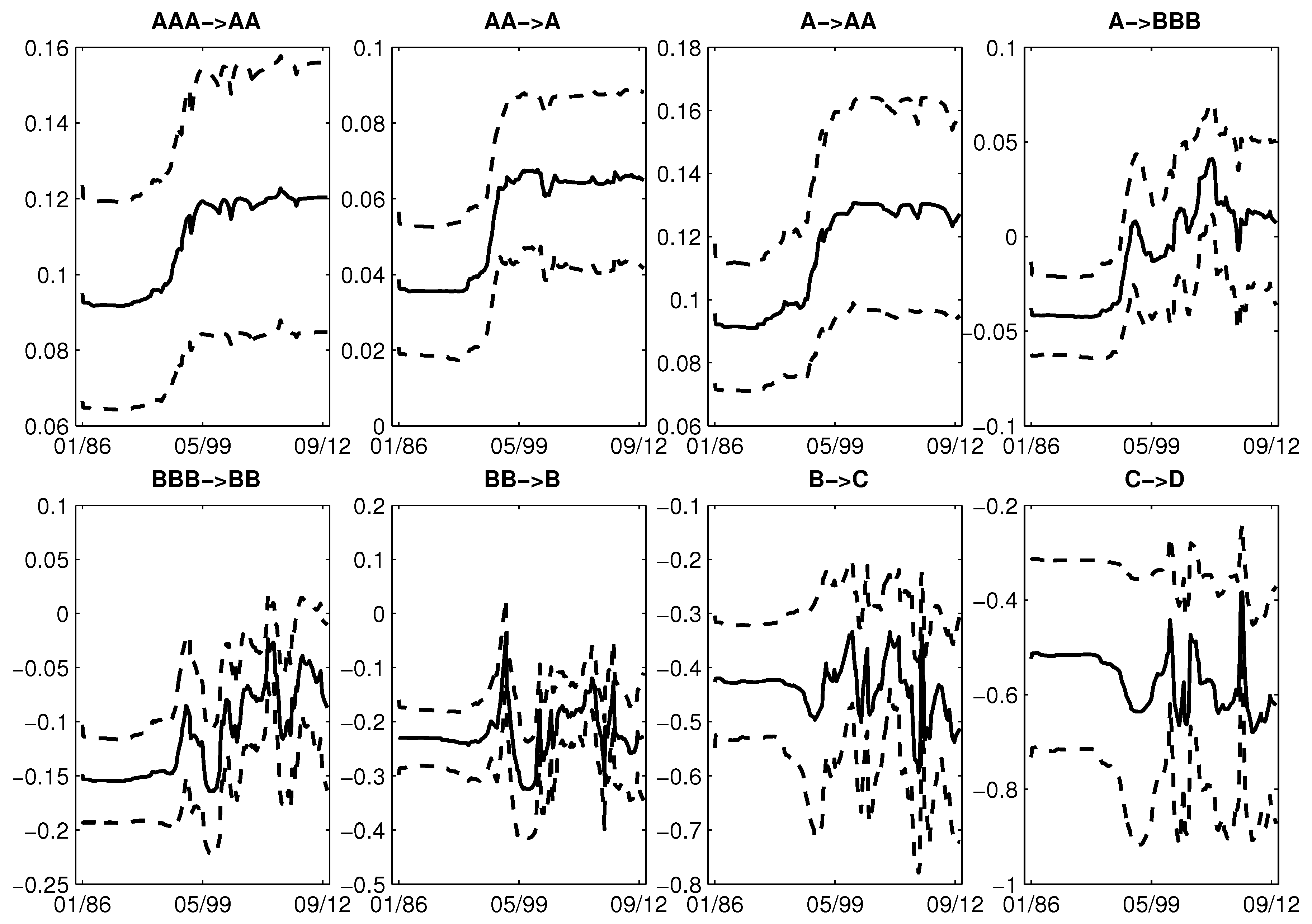
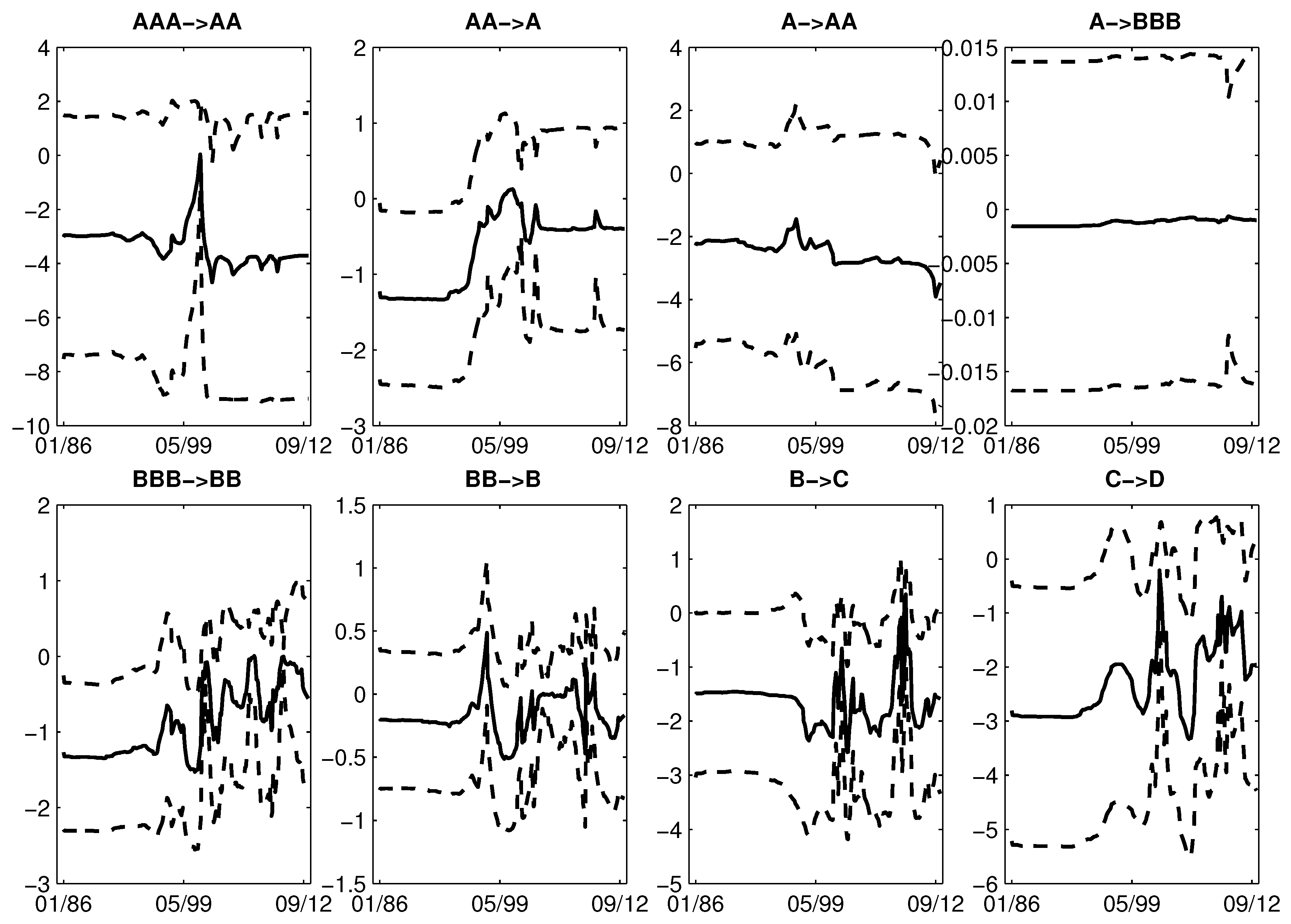
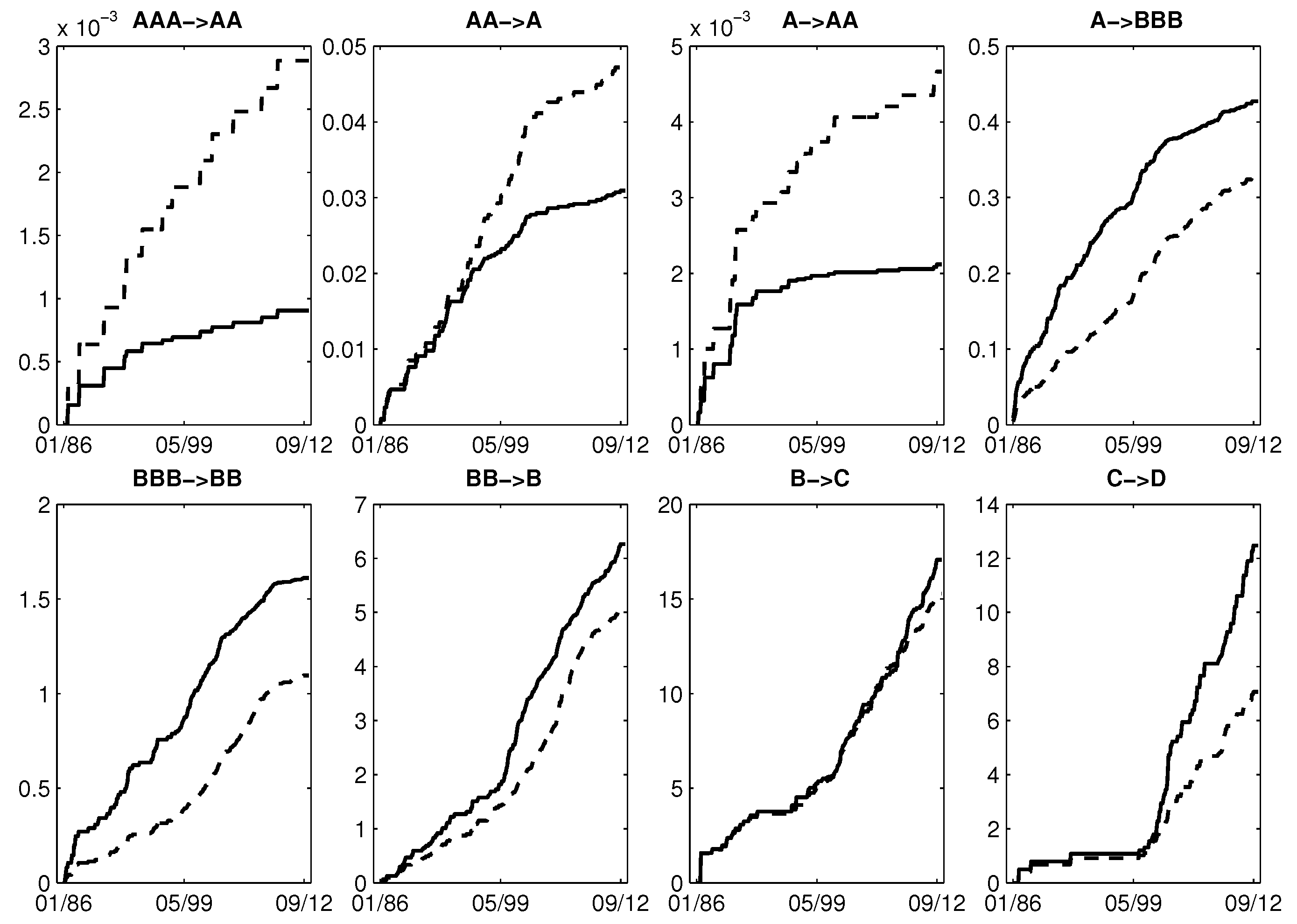
5.3. Firms’ Rating Transition Intensities and Probabilities

With the estimated ${\mathit{\theta }}^{(i,j)}(t)$ and baseline intensities, we can use Equations (4) and (5) to compute all types of rating transition intensities for each firm and furthermore the rating transition probabilities. Note that the firm’s intensities given by Equations (4) and (5) are the mean functions after integrating all random effects. For example, for the Costco Wholesale Corporation, Figure 4 plots the estimated mean functions of cumulative intensities for different rating transitions with (solid) and without (dashed) the assumptions of structural breaks. We notice that, for some rating transition types such as $\mathcal{AAA}\to \mathcal{AA}$, $\mathcal{AA}\to \mathcal{A}$ and $\mathcal{A}\to \mathcal{AA}$, the cumulative intensities of Costco under structural breaks assumption are smaller than the ones without structural breaks assumption, while larger for other transitions types such as $\mathcal{BB}\to \mathcal{B}$ and $\mathcal{C}\to \mathcal{D}$, which is contrary to the finding for baseline cumulative intensities. This further confirms the significant effect of firms’ covariates on firms’ rating transitions.

We further compute Costco’s transition probability matrices for different periods and with different assumptions. The first panel of

Table 1. Estimated transition probability matrices of the Costco Wholesale Corporation.

	$\mathcal{AAA}$	$\mathcal{AA}$	$\mathcal{A}$	$\mathcal{BBB}$	$\mathcal{BB}$	$\mathcal{B}$	$\mathcal{CCC}$	$\mathcal{D}$
January 1986–September 2012 (without structural break assumption)
$\mathcal{AAA}$	0.9993	7 × 10${}^{-4}$	3 × 10${}^{-6}$	2 × 10${}^{-8}$	2 × 10${}^{-10}$	2 × 10${}^{-11}$	1 × 10${}^{-12}$	2 × 10${}^{-14}$
$\mathcal{AA}$	1 × 10${}^{-4}$	0.9927	7 × 10${}^{-3}$	9 × 10${}^{-5}$	8 × 10${}^{-7}$	1 × 10${}^{-7}$	9 × 10${}^{-9}$	1 × 10${}^{-10}$
$\mathcal{A}$	9 × 10${}^{-8}$	0.0012	0.9742	0.0241	3 × 10${}^{-4}$	5 × 10${}^{-5}$	5 × 10${}^{-6}$	1 × 10${}^{-7}$
$\mathcal{BBB}$	3 × 10${}^{-10}$	6 × 10${}^{-6}$	0.0098	0.9577	0.0274	0.0043	6 × 10${}^{-4}$	2 × 10${}^{-5}$
$\mathcal{BB}$	1 × 10${}^{-12}$	4 × 10${}^{-8}$	9 × 10${}^{-5}$	0.0183	0.9173	0.0552	0.0087	2 × 10${}^{-4}$
$\mathcal{B}$	7 × 10${}^{-15}$	3 × 10${}^{-10}$	8 × 10${}^{-7}$	2 × 10${}^{-4}$	0.0219	0.7215	0.2463	0.0100
$\mathcal{CCC}$	3 × 10${}^{-17}$	1 × 10${}^{-12}$	5 × 10${}^{-9}$	2 × 10${}^{-6}$	3 × 10${}^{-4}$	0.0208	0.9066	0.0722
October 1994–March 2001 (with structural break assumption)
$\mathcal{AAA}$	0.9998	2 × 10${}^{-4}$	3 × 10${}^{-7}$	6 × 10${}^{-10}$	2 × 10${}^{-13}$	1 × 10${}^{-14}$	2 × 10${}^{-20}$	5 × 10${}^{-24}$
$\mathcal{AA}$	2 × 10${}^{-5}$	0.9968	0.0031	1 × 10${}^{-5}$	5 × 10${}^{-9}$	3 × 10${}^{-10}$	5 × 10${}^{-16}$	2 × 10${}^{-19}$
$\mathcal{A}$	3 × 10${}^{-9}$	3 × 10${}^{-4}$	0.9933	0.0063	4 × 10${}^{-6}$	2 × 10${}^{-7}$	6 × 10${}^{-13}$	2 × 10${}^{-16}$
$\mathcal{BBB}$	4 × 10${}^{-12}$	7 × 10${}^{-7}$	0.0041	0.9944	0.0013	8 × 10${}^{-5}$	3 × 10${}^{-10}$	9 × 10${}^{-14}$
$\mathcal{BB}$	5 × 10${}^{-15}$	1 × 10${}^{-9}$	1 × 10${}^{-5}$	0.0055	0.9935	0.0010	4 × 10${}^{-9}$	1 × 10${}^{-12}$
$\mathcal{B}$	3 × 10${}^{-18}$	9 × 10${}^{-12}$	1 × 10${}^{-8}$	8 × 10${}^{-6}$	0.0028	0.9971	8 × 10${}^{-6}$	2 × 10${}^{-9}$
$\mathcal{CCC}$	2 × 10${}^{-23}$	7 × 10${}^{-18}$	1 × 10${}^{-13}$	1 × 10${}^{-10}$	6 × 10${}^{-8}$	4 × 10${}^{-5}$	0.9999	4 × 10${}^{-9}$
April 2007–January 2010 (with structural break assumption)
$\mathcal{AAA}$	0.9999	1 × 10${}^{-4}$	1 × 10${}^{-8}$	7 × 10${}^{-12}$	3 × 10${}^{-15}$	3 × 10${}^{-17}$	5 × 10${}^{-23}$	9 × 10${}^{-27}$
$\mathcal{AA}$	7 × 10${}^{-6}$	0.9998	0.0002	2 × 10${}^{-7}$	1 × 10${}^{-10}$	1 × 10${}^{-12}$	2 × 10${}^{-18}$	4 × 10${}^{-22}$
$\mathcal{A}$	9 × 10${}^{-11}$	3 × 10${}^{-5}$	0.9981	0.0018	2 × 10${}^{-6}$	1 × 10${}^{-8}$	4 × 10${}^{-14}$	8 × 10${}^{-18}$
$\mathcal{BBB}$	4 × 10${}^{-14}$	1 × 10${}^{-8}$	0.0011	0.9972	0.0017	2 × 10${}^{-5}$	6 × 10${}^{-11}$	1 × 10${}^{-14}$
$\mathcal{BB}$	2 × 10${}^{-17}$	1 × 10${}^{-11}$	1 × 10${}^{-6}$	0.0023	0.9967	9 × 10${}^{-4}$	4 × 10${}^{-9}$	8 × 10${}^{-13}$
$\mathcal{B}$	7 × 10${}^{-21}$	5 × 10${}^{-15}$	7 × 10${}^{-10}$	2 × 10${}^{-6}$	0.0016	0.9984	8 × 10${}^{-6}$	2 × 10${}^{-9}$
$\mathcal{CCC}$	1 × 10${}^{-25}$	8 × 10${}^{-20}$	2 × 10${}^{-14}$	6 × 10${}^{-11}$	7 × 10${}^{-8}$	9 × 10${}^{-5}$	0.9999	1 × 10${}^{-5}$

shows the estimated transition probability matrix for the whole sample period without structural break assumption, and the second and third panels show the estimated matrices for two periods with the structural break assumption. We chose these two periods because both the estimated baseline and Costco’s cumulative intensities show big shifts around these periods. We found that the transition probabilities from non-default ratings to the default state are much smaller when the assumption of market structural break is incorporated.

6. Concluding Remarks

There have been many studies on how firms’ credit risk depends on risk factors, which are usually summarized as observed or latent time series in reduced-form models of firms’ credit risk. During the past decades, it was noticed that structural breaks or crisis in the financial market also have significant impact on firms’ credit risk. However, modeling such effects is not easy, as structural breaks in the market cannot be simply summarized as observed or latent time series (or risk factors). To address this issue and incorporate the impact of market structural breaks on firm’s credit risk, we propose a modulated semi-Markov model with unknown structural breaks to characterize the relationship of firms’ credit rating transitions and firms’ covariates in the presence of unobserved market structural breaks. We assume that, in our model, the number, locations, and magnitude of structural breaks are unknown, which maximally mimics structural breaks in the market. Given the fact that traditional inference procedures are not applicable here due to the complicated mechanism of market structural breaks, we use a mixed estimating equation approach to estimate the time-varying regression coefficients that represent the effect of market structural breaks, baseline rating transition intensities for all firms and rating transition intensities for individual firms. The proposed inference procedure is not only simple to implement, but also has nice asymptotic properties. We use the developed model and inference procedure to analyze U.S. firms’ rating records and related firms’ risk factors (distance to default and trailing returns) from 1986 to 2012, and show that the relationship of firms’ credit risk and firms’ covariates does undergo sudden shifts when market structural break occurs.

Besides modeling the firms’ credit rating transitions in the presence of market structural breaks, our model also suggests a way to aggregates firm’s credit history, their accounting records, and variations of market into a single model. This allows us to study further the impact of other or more complicated risk factors on firms’ credit risk when market varies. For example, the current study ignores the dynamic feature of risk factors and the feedback effect of changes of firms’ credit risk, which should be investigated in further studies. The proposed model also has some limits. For instance, as the model assumes that macroeconomic information is independent of firms’ behavior, it fails to handle market structural breaks due to failures of one or several “too-big-to-fall" firms; issues such as this should be studied further.

References

1. Altman, Edward I. 1968. Financial ratios, discriminant analysis and the prediction of corporate bankruptcy. Journal of Finance 23: 589–609. [Google Scholar] [CrossRef]
2. Andersen, Per K., and Richard D. Gill. 1982. Cox’s regression model for counting processes: A large sample study. Annals of Statistics 10: 1100–20. [Google Scholar] [CrossRef]
3. Beaver, William H. 1968. The information content of annual earnings announcements. Journal of Accounting Research 6: 67–92. [Google Scholar] [CrossRef]
4. Black, Fischer, and John C. Cox. 1976. Valuing corporate securities: Some effects of bond indenture provisions. Journal of Finance 31: 351–67. [Google Scholar] [CrossRef]
5. Black, Fischer, and Myron Scholes. 1973. The pricing of options and corporate liabilities. Journal of Political Economy 81: 637–59. [Google Scholar] [CrossRef]
6. Briys, Eric, and François De Varenne. 1997. Valuing risky fixed rate debt: An extension. Journal of Financial and Quantitative Analysis 32: 239–48. [Google Scholar] [CrossRef]
7. Buonocore, Aniello, Amelia G. Nobile, and Luigi M. Ricciardi. 1987. A new integral equation for the evaluation of first-passage-time probability densities. Advances in Applied Probability 19: 784–800. [Google Scholar] [CrossRef]
8. Chava, Sudheer, and Robert A. Jarrow. 2004. Bankruptcy prediction with industry effects. Review of Finance 8: 537–69. [Google Scholar] [CrossRef]
9. Collin-Dufresne, Pierre, and Robert S. Goldstein. 2001. Do credit spreads reflect stationary leverage ratios? Journal of Finance 56: 1929–57. [Google Scholar] [CrossRef]
10. Dionne, Georges, Geneviѐve Gauthier, Khemais Hammami, Mathieu Maurice, and Jean-Guy Simonato. 2011. A reduced form model of default spreads with Markov-switching macroeconomic factors. Journal of Banking and Finance 35: 1984–2000. [Google Scholar] [CrossRef] [Green Version]
11. Duffie, Darrell, and David Lando. 2001. Term structures of credit spreads with incomplete accounting information. Econometrica 69: 633–64. [Google Scholar] [CrossRef]
12. Duffie, Darrell, Leandro Saita, and Ke Wang. 2007. Multi-period corporate default prediction with stochastic covariates. Journal of Financial Economics 83: 635–65. [Google Scholar] [CrossRef]
13. Duffie, Darrell, Andreas Eckner, Guillaume Horel, and Leandro Saita. 2009. Frailty correlated default. Journal of Finance 64: 2089–123. [Google Scholar] [CrossRef]
14. Fisher, Edwin O., Robert Heinkel, and Josef Zechner. 1989. Dynamic capital structure choice: Theory and tests. Journal of Finance 44: 19–40. [Google Scholar] [CrossRef]
15. Hilberink, Bianca, and Chris L. Rogers. 2002. Optimal capital structure and endogenous default. Finance and Stochastics 6: 237–63. [Google Scholar] [CrossRef]
16. Hillegeist, Stephen A., Elizabeth K. Keating, Donald P. Cram, and Kyle G. Lundstedt. 2004. Assessing the probability of bankruptcy. Review of Accounting Studies 9: 5–34. [Google Scholar] [CrossRef]
17. Kalbfleisch, John D., and Ross L. Prentice. 2002. The Statistical Analysis of Failure Time Data. New York: Weily. [Google Scholar]
18. Koopman, Siem J., André Lucas, and André Monteiro. 2008. The multi-state latent factor intensity model for credit rating transitions. Journal of Econometrics 142: 399–424. [Google Scholar] [CrossRef] [Green Version]
19. Koopman, Siem J., André Lucas, and Bernd Schwabb. 2010. Macro, Frailty and Contagion Effects in Defaults: Lessons from the 2008 Credit Crisis. Working pape. Amsterdam, The Netherlands: University of Amsterdam. [Google Scholar]
20. Lee, Suk Hun, and Jorge L. Urrutia. 1996. Analysis and prediction of insolvency in the property-liability insurance industry: A comparison of logit and hazard models. Journal of Risk and Insurance 63: 121–30. [Google Scholar] [CrossRef]
21. Leland, Hayne E. 1994. Corporate debt value, bond covenants, and optimal capital structure. Journal of Finance 49: 1213–52. [Google Scholar] [CrossRef]
22. Lin, Danyu, Lee-Jen Wei, I. Yang, and Zhiliang Ying. 2000. Semiparametric regression for the mean and rate functions of recurrent events. Journal of the Royal Statistical Society: Series B 62: 711–30. [Google Scholar] [CrossRef]
23. McDonald, Cynthia G., and Linda M. Van de Gucht. 1999. High-yield bond default and call risks. Review of Economics and Statistics 81: 409–19. [Google Scholar] [CrossRef]
24. Merton, Robert C. 1974. On the pricing of corporate debt: The risk structure of interest rates. Journal of Finance 29: 449–70. [Google Scholar]
25. Minsky, Hayman P. 1982. Can It Happen Again? Armonk: ME Sharpe. [Google Scholar]
26. Minsky, Hayman P. 1986. Stabilizing an Unstable Economy. New Haven: Yale University Press. [Google Scholar]
27. Shumway, Tyler. 2001. Forecasting bankrupcty more accurately: A simple hazard model. Journal of Business 74: 101–24. [Google Scholar] [CrossRef]
28. Xing, Haipeng, and Ying Chen. 2018. Dependence of structural breaks in rating transition dynamics on economic and market variations. Review of Economics and Finance 11: 1–18. [Google Scholar]
29. Xing, Haipeng, and Zhiliang Ying. 2012. A semiparametric change-point regression model for longitudinal observations. Journal of the American Statistical Association 107: 1625–37. [Google Scholar] [CrossRef]
30. Xing, Haipeng, Ning Sun, and Ying Chen. 2012. Credit rating dynamics in the presence of unknown structural breaks. Journal of Banking and Finance 36: 78–89. [Google Scholar] [CrossRef]
Figure 1. θ ^ 1 ( i , j ) ( t ) (solid) and their 95% confidence bands (dotted) for firms’ distance to default. Note that the values of θ ^ 1 ( i , j ) for the corresponding transitions (from left to right and top to down) are 0.069, 0.039, 0.075, −0.004, −0.102, −0.204, −0.426, and −0.378, respectively.
Risks 06 00136 g001
Figure 2. θ ^ 2 ( i , j ) ( t ) (solid) and their 95% confidence bands (dotted) for firms’ trailing returns. Note that the values of θ ^ 2 ( i , j ) for the corresponding transitions (from left to right and top to down) are −1.695, −0.135, −1.277, −0.001, −1.272, −1.088, −1.164, and −4.052, respectively.
Risks 06 00136 g002
Figure 3. Estimated baseline cumulative intensities with (solid) and without (dashed) structural breaks.
Risks 06 00136 g003
Figure 4. Mean functions of the Costco Wholesale Corporation’s cumulative intensities.
Risks 06 00136 g004