Application of Machine Learning to Mortality Modeling and Forecasting

Abstract

Estimation of future mortality rates still plays a central role among life insurers in pricing their products and managing longevity risk. In the literature on mortality modeling, a wide number of stochastic models have been proposed, most of them forecasting future mortality rates by extrapolating one or more latent factors. The abundance of proposed models shows that forecasting future mortality from historical trends is non-trivial. Following the idea proposed in Deprez et al. (2017), we use machine learning algorithms, able to catch patterns that are not commonly identifiable, to calibrate a parameter (the machine learning estimator), improving the goodness of fit of standard stochastic mortality models. The machine learning estimator is then forecasted according to the Lee-Carter framework, allowing one to obtain a higher forecasting quality of the standard stochastic models. Out-of sample forecasts are provided to verify the model accuracy.

1. Introduction

During the 20th Century, mortality has declined at all ages, producing a steep increase in life expectancy. This decrease is mainly due to the reduction of infectious disease mortality (between 1900 and 1950), as well as cardio-circulatory diseases and cancer mortality (in the most recent decades). Knowledge of future mortality rates is an important matter for life insurance companies with the goal of achieving adequate pricing of their life products. Therefore, sophisticated techniques to forecast future mortality rates have become increasingly popular in actuarial science, in order to deal with the longevity risk. Among the stochastic mortality models proposed in the literature, the Lee-Carter model Lee and Carter (1992) is the most widely used in the world, probably for its robustness. The original model applies singular-value decomposition (SVD) to the log-force of mortality to find three latent parameters: a fixed age component and a time component capturing the mortality trend that is multiplied by an age-specific function. Then, the time component is forecasted using a random walk. More recent approaches involve non-linear regression and generalized linear models (GLM), e.g., Brouhns et al. (2002) assumed a Poisson distribution for deaths and calculated the Lee-Carter model parameters by log-likelihood maximization.

In recent years, machine learning techniques have assumed an increasingly central role in many areas of research, from computer science to medicine, including actuarial science. Machine learning is an application of artificial intelligence through a series of algorithms that are optimized on data samples or previous experience. That is, given a certain model defined as a function of a group of parameters, learning consists of improving these parameters using datasets or accumulated experience (the “training data”). Even though machine learning may not explain everything, it is very useful in detecting patterns, even unknown and unidentifiable ones, as well as hidden correlations. In this way, it allows us to understand processes better, make predictions about the future based on historical data, and categorize sets of data automatically.

We can distinguish between supervised and unsupervised learning methods. In the supervised learning methods, the goal is to establish the relations between a range of predictors (independent variables) and a determined target (dependent variable), whereas in the unsupervised learning methods, the algorithm sets patterns among a range of variables in order to group records that show similarities, without considering an output measure. While in the supervised method, the algorithm learns from the dataset the rules that are fed to the machine, in the unsupervised method, it has to identify the rules autonomously. Logistic and multiple regression, classification and regression trees, and naive Bayes are examples of supervised learning methods, while association rules and clustering are classified as unsupervised learning methods.

Despite the increasing usage in different fields of research, applications of machine learning in demography are not so popular. The main reason lies in the findings often being seen as “black boxes” and considered difficult to interpret. Moreover, the algorithms are not theory driven (but quite data driven), while demographers are often interested in analyzing specific hypotheses. They are likely to be unwilling to use algorithms whose decisions cannot be rationally explained.

However, we believe that machine learning techniques can be valuable as a complement to standard mortality models, rather than a substitute.

In the literature related to mortality modeling, there are very few contributions on this topic. The work in Deprez et al. (2017) showed that machine learning algorithms are useful to assess the goodness of fit of the mortality estimates provided by standard stochastic mortality models (they considered Lee-Carter and Renshaw-Haberman models). They applied a regression tree boosting machine to “analyze how the modeling should be improved based on feature components of an individual, such as its age or its birth cohort. This (non-parametric) regression approach then allows us to detect the weaknesses of different mortality models” (p. 337). In addition, they investigated cause-of-death mortality. In a recent paper, the work in Hainaut (2018) used neural networks to find the latent factors of mortality and forecast them according to a random walk with drift. Finally, the work in Richman and Wüthrich (2018) extended the Lee-Carter model to multiple populations using neural networks.

We investigate the ability of machine learning to improve the accuracy of some standard stochastic mortality models, both in the estimation and forecasting of mortality rates. The novelty of this paper is primarily in the mortality forecasting that takes advantage of machine learning, clearly capturing patterns that are not identifiable with a standard mortality model. Following Deprez et al. (2017), we use tree-based machine learning techniques to calibrate a parameter (the machine learning estimator) to be applied to mortality rates fitted by the standard mortality model.

We analyze three famous stochastic mortality models: the Lee-Carter model Lee and Carter (1992), which is still the most frequently implemented, the Renshaw-Haberman model Renshaw and Haberman (2006), which also considers the cohort effect, and the Plat model Plat (2009), which tries to combine the parameters of the Lee-Carter model with those of the Cairns-Blake-Dowd model with the cohort effect, named “M7” (Cairns et al. (2009)).

Three different kinds of supervised learning methods are considered for calibrating the machine learning estimator: decision tree, random forest, and gradient boosting, which are all tree-based.

We show that the implementation of these machine learning techniques, based on features components such as age, sex, calendar year, and birth cohort, leads to a better fit of the historical data, with respect to the estimates given by the Lee-Carter, Renshaw-Haberman, and Plat models. We also apply the same logic to improve the mortality forecasts provided by the Lee-Carter model, where the machine learning estimator is extrapolated using the Lee-Carter framework. Out-of-sample tests are performed for the improved model in order to verify the quality of forecasting.

The paper is organized as follows. In Section 2, we specify the model and introduce the tree-based machine learning estimators. In Section 3, we present the stochastic mortality models considered in the paper. In Section 4, we illustrate the usage of tree-based machine learning estimators to improve both the fitting and forecasting quality of the original mortality models. Conclusions and further research are then given in Section 5.

2. The Model

We consider the following categorical variables, identifying an individual: gender (g), age (a), calendar year (t), and year of birth (c). We assign to each individual the feature $\mathbf{x}=(g,a,t,c)\in \mathcal{X}$ with $\mathcal{X}=\mathcal{G}\times \mathcal{A}\times \mathcal{T}\times \mathcal{C}$ the feature space, where: $\mathcal{G}=\left\{males,females\right\}$, $\mathcal{A}=\left\{0,\dots ,\omega \right\}$, $\mathcal{T}=\left\{t_1,\dots ,t_n\right\}$, $\mathcal{C}=\left\{c_1,\dots ,c_m\right\}$. Other categorical variables could be included in the feature space X, e.g., the marital status, the income, and other individual information.

We assume that the number of deaths $D_{\mathbf{x}}$ meets the following conditions:

• $D_{\mathbf{x}}$ are independent in $\left\{\mathbf{x}\in \mathcal{X}\right\}$;
• $D_{\mathbf{x}}\sim Pois(m_{\mathbf{x}}·E_{\mathbf{x}})$ for all $\left\{\mathbf{x}\in \mathcal{X}\right\}$.

where $m_{\mathbf{x}}$ is the central death rate and $E_{\mathbf{x}}$ are the exposures.

Let us define $d_{\mathbf{x}}^{\mathrm{mdl}}$ as the expected number of deaths estimated by a standard stochastic mortality model (such as Lee-Carter, Cairns-Blake-Dowd, etc.) and $m_{\mathbf{x}}^{\mathrm{mdl}}$ the corresponding central death rate. Following Deprez et al. (2017), but modeling the central death death rate instead of mortality rate ($q_{\mathbf{x}}$), we initially set:

• $m_{\mathbf{x}}=m_{\mathbf{x}}^{\mathrm{mdl}}$
• $D_{\mathbf{x}}\sim Pois({\psi }_{\mathbf{x}}·d_{\mathbf{x}}^{\mathrm{mdl}}),\mathrm{with}{\psi }_{\mathbf{x}}\equiv 1,d_{\mathbf{x}}^{\mathrm{mdl}}=m_{\mathbf{x}}^{\mathrm{mdl}}{E}_{\mathbf{x}}$

The condition ${\psi }_{\mathbf{x}}\equiv 1$ means that the specified mortality model perfectly fits the crude rates. However, in the real world, a mortality model could overestimate (${\psi }_{\mathbf{x}}\le 1$) or underestimate (${\psi }_{\mathbf{x}}\ge 1$) the crude rates. Therefore, we calibrate the parameter ${\psi }_{\mathbf{x}}$, based on the feature $\mathbf{x}$, according to three different machine learning techniques. We find ${\psi }_{\mathbf{x}}$ as a solution of a regression tree algorithm applied to the ratio between the death observations and the corresponding value estimated by the specified mortality model $\frac{D_{\mathbf{x}}}{d_{\mathbf{x}}^{\mathrm{mdl}}}$:

$$\frac{D_{\mathbf{x}}}{d_{\mathbf{x}}^{\mathrm{mdl}}}\sim \mathsf{gender}+\mathsf{age}+\mathsf{year}+\mathsf{cohort}$$

(1)

We denote by ${\widehat{\psi }}_{\mathbf{x}}^{\mathrm{mdl},\mathrm{ML}}$ the machine learning estimator obtained by solving Equation (1), where mdl indicates the stochastic mortality model and ML the machine learning algorithm used to improve the mortality rates given by a certain model. The estimator ${\widehat{\psi }}_{\mathbf{x}}^{\mathrm{mdl},\mathrm{ML}}$ is then applied to the central death rate of the specified mortality model, $m_{\mathbf{x}}^{\mathrm{mdl}}$, aiming to obtain a better fit of the observed data:

$$m_{\mathbf{x}}^{\mathrm{mdl},\mathrm{ML}}={\widehat{\psi }}_{\mathbf{x}}^{\mathrm{mdl},\mathrm{ML}}·m_{\mathbf{x}}^{\mathrm{mdl}},\forall \mathbf{x}\in \mathcal{X}$$

(2)

As in Deprez et al. (2017), we measure the improvement in the mortality rates attained by the tree growing algorithm through the relative changes of central death rates:

$$\Delta m_{\mathbf{x}}^{\mathrm{mdl},\mathrm{ML}}=\frac{m_{\mathbf{x}}^{\mathrm{mdl},\mathrm{ML}}-m_{\mathbf{x}}^{\mathrm{mdl}}}{m_{\mathbf{x}}^{\mathrm{mdl}}}={\widehat{\psi }}_{\mathbf{x}}^{\mathrm{ML}}-1$$

(3)

The work in Hainaut (2018) used neural networks to learn the logarithm of the central death rates directly from the features of the mortality data, by using age, calendar year, and gender (and region) as predictors in a neural network. We instead rely on the classical form of the Lee-Carter model that we improve ex-post using machine learning algorithms, considered complementary and not an alternative to the standard mortality modeling.

To estimate ${\widehat{\psi }}_{\mathbf{x}}^{\mathrm{mdl},\mathrm{ML}}$, we use the following tree-based machine learning (ML) techniques:

• Decision tree
• Random forest
• Gradient boosting

2.1. Decision Trees

The tree-based methods for regression and classification (Breiman et al. 1984) have become popular alternatives to linear regression. They are based on the partition of the feature space $\mathcal{X}$, through a sequence of binary splits, and the set of splitting rules used to segment the predictor space can be summarized in a tree (Hastie et al. 2016). Once the entire feature space is split into a certain number of simple regions recursively, the response for a given observation can be predicted using the mean of the training observations in the region to which that observation belongs (James et al. 2017; Alpaydin 2010).

Let ${({\mathcal{X}}_{\tau })}_{\tau \in \mathcal{T}}$ be the partition of $\mathcal{X}$; the decision tree estimator is calculated as:

$$\widehat{\psi }(\mathbf{x})=\sum _{\tau \in \mathcal{T}}{\overline{\psi }}_{\tau }{\mathbb{1}}_{\{\mathbf{x}\in {\mathcal{X}}_{\tau }\}}$$

(4)

Decision trees (DT) algorithms have advantages over other types of regression models. As pointed out by James et al. (2017): they are easy to interpret; they can easily handle qualitative predictors without the need to create dummy variables; they can catch any kind of correlation in the data. However, they suffer from some important drawbacks: they do not always have predictive accuracy levels similar to those of traditional regression and classification models; they can lack robustness: a small modification of the data can produce a tree that strongly differs from the one initially estimated.

The ML estimator is obtained using the R package rpart (Therneau and Atkinson 2017). The algorithm provides the estimate of $\widehat{\psi }(\mathbf{x})$ given by the average of the response variable values $\psi (\mathbf{x})$ belonging to the same region identified by the regression tree. The values of the complexity parameter ($cp$) for the decision trees are chosen with the aim of making the number of splits considered uniform.

2.2. Random Forest

The aggregation of many decision trees can improve the predictive performance of trees. Therefore, we first apply bagging (also called bootstrap aggregation) to produce a certain number, B, of decision trees from the bootstrapped training samples, in turn obtained from the bootstrap of the original training dataset. Random forest (RF) differs from bagging in the way of considering the predictors: RF algorithms account only for a random subset of the predictors at each split in the tree, as described in detail by Breiman (2001). If there is a strong predictor in the dataset, the other predictors will have more of a chance to be chosen as split candidates from the final set of predictors (James et al. 2017). The RF estimator is calculated as follows:

$$\widehat{\psi }(\mathbf{x})=\frac{1}{B}\sum _{b=1}^B{\widehat{\psi }}^{(b)}(\mathbf{x})$$

(5)

The RF estimator is obtained by applying the algorithm from the R package randomForest (Liaw 2018). Since this procedure proved to be very costly from a computational point of view, the number of trees must be carefully chosen: it should not be too large, but at the same time able to produce an adequate percentage of variance explained and a low mean of squared residuals, MSR.

2.3. Gradient Boosting

Consider the loss in using a certain function to predict a variable on the training data; gradient boosting (GB) aims at minimizing the in-sample loss with respect to this function by a stage-wise adaptive learning algorithm that combines weak predictors.

Let $\psi (\mathbf{x})$ be the function; the gradient boosting algorithm finds an approximation $\widehat{\psi }(\mathbf{x})$ to the function $\psi (\mathbf{x})$ that minimizes the expected value of the specified differentiable loss function (optimization problem). At each stage i of gradient boosting ($1\le i\le N$), we suppose that there is some imperfect models $\widehat{\psi }({\mathbf{x}}_i)$, then the gradient boosting algorithm improves on $\widehat{\psi }({\mathbf{x}}_i)$ by constructing a new model that adds an estimator h to provide a better model:

$$\widehat{\psi }({\mathbf{x}}_i)=\widehat{\psi }({\mathbf{x}}_{i-1})+{\lambda }_i{h}_i(\mathbf{x})$$

(6)

where $h_i\in \mathcal{H}$ is a base learner function ($\mathcal{H}$ is the set of arbitrary differentiable functions) and $\lambda$ is a multiplier obtained by solving the optimization problem. The GB estimator is obtained using the R package gbm (Ridgeway 2007). The gbm package requires choosing the number of trees ($n.trees$) and other key parameters as the number of cross-validation folds ($cv.folds$), the depth of each tree involved in the estimate ($interaction.depth$), and the learning rate parameter ($shrinkage$). The number of trees, representing the number of GB iterations, must be accurately chosen, as a high number would reduce the error on the training set, while a low number would result in overfitting. The number of cross-validation folds to perform should be chosen according to the dataset size. In general, five-fold cross-validation, which corresponds to $20\%$ of the data involved in testing, is considered a good choice in many cases. Finally, the interaction depth represents the highest level of variable interactions allowed or the maximum nodes for each tree.

3. Mortality Models

Let us consider the generalized age period cohort (GAPC) stochastic mortality models’ family (see Villegas et al. 2015 for further details). In the GAPC models, the effects of age, calendar year, and cohort are caught by a predictor, in our framework denoted by ${\eta }_{\mathbf{x}}$, as follows:

$${\eta }_{\mathbf{x}}={\alpha }_a+\sum _{i=1}^n{\beta }_a^{(i)}{\kappa }_t^{(i)}+{\beta }_a^{(0)}{\gamma }_{t-a},\forall \mathbf{x}=(g,a,t,c)\in \mathcal{X}$$

(7)

where:

• ${\alpha }_a$: age-specific parameter providing the average age profile of mortality;
• ${\beta }_a^{(i)}·{\kappa }_t^{(i)}$, $\forall i$: age-period terms describing the mortality trends (${\kappa }_t^{(i)}$ is the time index, and ${\beta }_a^{(i)}$ modifies the effect of ${\kappa }_t^{(i)}$ across ages);
• ${\beta }_a^{(0)}·{\gamma }_{t-a}$: represents the cohort effect, where ${\gamma }_{t-a}$ is the cohort parameter and ${\beta }_a^{(0)}$ modifies its effect across ages ($c=t-a$ is the year of birth).

The mortality predictor is related to a link function g, so that: ${\eta }_{\mathbf{x}}=g\left(\mathbb{E}\left(\frac{D_{\mathbf{x}}}{E_{\mathbf{x}}}\right)\right)$. In this paper, we consider the log link function and assume that the numbers of deaths $D_{\mathbf{x}}$ follow a Poisson distribution.

3.1. Lee-Carter Model

Under the above-described framework, the Lee-Carter (LC) model as proposed by Brouhns et al. (2002) requires a log link function to target the central death rate. In the LC model, the logarithm of the central death rate is described by:

$$log\left(m_{\mathbf{x}}\right)={\alpha }_a+{\beta }_a^{(1)}{\kappa }_t^{(1)}$$

(8)

with the constraints: ${\sum }_{t\in \mathcal{T}}{\kappa }_t^{(1)}=0$, ${\sum }_{a\in \mathcal{A}}{\beta }_a^{(1)}=1$ to avoid identifiability problems with the parameters. In order to forecast mortality with the LC model, the time index ${\kappa }_t^{(1)}$ is modeled by an autoregressive integrated moving average (ARIMA) process. In general, a random walk with drift properly fits the data:

$${\kappa }_t^{(1)}={\kappa }_{t-1}^{(1)}+\delta +{ϵ}_t,{ϵ}_t\sim N(0,{\sigma }_k^2)$$

(9)

where $\delta$ is the drift parameter and ${ϵ}_t$ are the error terms, normally distributed with null mean and variance ${\sigma }_k^2$.

3.2. Renshaw-Haberman Model

The Renshaw-Haberman model (Renshaw and Haberman (2006)) extends the LC model by including a cohort effect. The model’s predictor has the following expression, where the log link function is used to target the central death rate:

$$log\left(m_{\mathbf{x}}\right)={\alpha }_a+{\beta }_a^{(1)}{\kappa }_t^{(1)}+{\beta }_a^{(0)}{\gamma }_{t-a}$$

(10)

According to Haberman and Renshaw (2011) and Hunt and Villegas (2015), we set ${\beta }_a^{(0)}=1$ $\forall a\in \mathcal{A}$, as the model is more stable with respect to the original version.

$$log\left(m_{\mathbf{x}}\right)={\alpha }_a+{\beta }_a^{(1)}{\kappa }_t^{(1)}+{\gamma }_{t-a}$$

(11)

The model is subject to the following constraints, where $c=t-a$: ${\sum }_{t\in \mathcal{T}}{\kappa }_t^{(1)}=0$, ${\sum }_{a\in \mathcal{A}}{\beta }_a^{(1)}=1$, and ${\sum }_{c\in \mathcal{C}}{\gamma }_c=0$. Parameters ${\kappa }_t^{(1)}$ and ${\gamma }_{t-a}$ are modeled by ARIMA processes, assuming the independence between them.

3.3. Plat Model

The Plat model Plat (2009) aims to combine M7 and LC models in order to obtain a model appropriate for the entire age range and for capturing the cohort effect, thus overcoming the disadvantages of the previous models.

$$log(m_{\mathbf{x}})={\alpha }_a+{\kappa }_t^{(1)}+{\kappa }_t^{(2)}(\overline{a}-a)+{\kappa }_t^{(3)}{(\overline{a}-a)}^{+}+{\gamma }_{t-a}$$

(12)

where ${(\overline{a}-a)}^{+}=max(\overline{a}-a,0)$. This model is obtained from Equation (7) by setting ${\beta }_a^{(1)}=1$, ${\beta }_a^{(2)}=\overline{a}-a$, ${\beta }_a^{(3)}={(\overline{a}-a)}^{+}$, and ${\beta }_a^{(0)}=1$ and using the log link function to target the central death rate.

The Plat model is subject to the following constraints: ${\sum }_t{\kappa }_t^{(1)}=0$, ${\sum }_t{\kappa }_t^{(2)}=0$, ${\sum }_t{\kappa }_t^{(3)}=0$, ${\sum }_{c\in \mathcal{C}}{\gamma }_c=0$, ${\sum }_{c\in \mathcal{C}}{\gamma }_{c}c=0$, ${\sum }_{c\in \mathcal{C}}{\gamma }_c{c}^2=0$. As described in Villegas et al. (2015): “the first three constraints ensure that the period indexes are centered around zero, while the last three constraints ensure that the cohort effect fluctuates around zero and has no linear or quadratic trend”.

4. Numerical Analysis

4.1. Model Fitting

We fit the Lee-Carter (LC), Renshaw-Haberman (RH) and Plat models on the Italian population. Data were downloaded from the Human Mortality Database (www.mortality.org), while model fitting was performed with StMoMo package provided by Villegas et al. (2015). The following sets of gender $\mathcal{G}$, ages $\mathcal{A}$, years $\mathcal{T}$, and cohort $\mathcal{C}$ were considered in the analysis:

$\mathcal{G}=\left\{males,females\right\}$, $\mathcal{A}=\left\{0,\dots ,100\right\}$, $\mathcal{T}=\left\{1915,\dots ,2014\right\}$, and $\mathcal{C}=\left\{1815,\dots ,2014\right\}$.

The model accuracy was measured by the Bayes information criterion (BIC) and the Akaike information criterion (AIC), which are measures generally used to evaluate the goodness of fit of mortality models1. Log-likelihood $\mathcal{L}$, AIC and BIC values are reported in

Table 1. Log-likelihood, AIC and BIC statistics for LC, RH and Plat model. Ages 0–100 and years 1915–2014, Italian population.

Gender:	Males			Females
Model:	LC	RH	Plat	LC	RH	Plat
$\nu$	300	499	496	300	499	496
$\mathcal{L}$	−643,226	−307,985	−875,549	−176,421	−137,098	−281,518
AIC (Rank)	1,287,051 (2)	616,967 (1)	1,752,089 (3)	353,442 (2)	275,193 (1)	564,028 (3)
BIC (Rank)	1,289,218 (2)	620,570 (1)	1,755,671 (3)	355,608 (2)	278,796 (1)	567,610 (3)

, from which we observe that the RH model fits the historical data very well. It has the highest BIC and AIC values for both genders, with respect to the other models; then, in order, the LC model and the Plat model.

The goodness of fit is also tested by the residuals analysis. From Figure 1, we can observe that the RH provided the best fit, despite the highest number of parameters. The LC model provided a good fit especially for the old-age population, while the Plat model provided the worst performance despite the high number of parameters involved.

4.2. Model Fitting Improved by Machine Learning

In the following, we specify the parameters used to calibrate the ML algorithms described in Section 2 using the rpart, randomForest, and gbm packages, respectively:

• ${\widehat{\psi }}_{\mathbf{x}}^{\mathrm{mdl},\mathrm{DT}}$ was estimated with the rpart package by setting: $cp$ = 0.003 (complexity parameter);
• ${\widehat{\psi }}_{\mathbf{x}}^{\mathrm{mdl},\mathrm{RF}}$ was estimated with the randomForest package by setting: $ntrees$ = 200 (number of trees). Since this procedure proved to be very costly from a computational point of view, we limited the number of trees to 200, in order to guarantee both an adequate percentage of variance explained by the model and a low mean of squared residuals, MSR (see

  Table 2. Explained variance and MSR by the RF algorithm for the LC, RH, and Plat model. Ages 0–100 and years 1915–2014, Italian population.

  Model	Explained Variance	MSR
  LC	96.25%	0.0263
  RH	86.48%	0.0057
  Plat	91.14%	0.0058

  );
• ${\widehat{\psi }}_{\mathbf{x}}^{\mathrm{mdl},\mathrm{GB}}$ is estimated with the gbm package by setting: $n.trees$ = 5000 (number of trees); $cv.folds$ = 5 (number of cross-validation folds); $interaction.depth$ = 6; $shrinkage$ = 0.001 (learning rate) according to the algorithm implementation speed. The parameter $cv.folds$ is used to estimate the optimal number of iterations through the function $gbm.perf$ (see Figure 2).

The level of improvement in central death rates resulting from the application of ML algorithms was measured by $\Delta m_{\mathbf{x}}^{\mathrm{mdl},\mathrm{ML}}$, the relative changes described in Equation (3).

Numerical results for the LC, RH, and Plat model combined with the tree-based ML algorithms are shown in Figure 3 for males. Similar results were obtained for females.

The white areas represent very small variations of $\Delta m_{\mathbf{x}}^{\mathrm{mdl},\mathrm{ML}}$, approximately around zero. Larger white areas were observed for gradient boosting applied to the LC and RH model. In all cases, there were also significant changes that were less prominent for the RH model that best fit the historical data. Many regions were identified by diagonal splits (highlighting a cohort effect), strengthening our choice to insert the cohort parameter in the decision tree algorithms.

Especially for the LC model, we point out that the relative changes were mainly concentrated in the young ages. For the Plat model, we observed small values of $\Delta m_{\mathbf{x}}^{\mathrm{PL},\mathrm{ML}}$ with respect to the other mortality models, with the exception of the population aged under 40 that showed quite significant changes. From these early results, DT and RT seemed to work better than the GB algorithm.

Since the most significant changes were concentrated in the younger ages, we show the mortality rates (in log scale) only for the age group 0–50 (Figure 4). For the sake of brevity, we show the results for the male population. Similar results were obtained for females and are reported in the Appendix (see Figure A1).

From the plots, we can argue that ML estimators led to an improvement in the quality of fit in all the mortality models considered. The plots show that the application of an ML estimator involves significant changes in the values of the mortality rate with a significant improvement in the fitting of the data. Among the stochastic mortality models considered here, the Plat model is the one that achieved the highest fit improvements from the use of ML algorithms.

Further, we measured the goodness of fit of the models with the mean absolute percent error (MAPE), defined as:

$$\mathrm{MAPE}=\frac{100}{N}\sum _{\mathbf{x}}\left|\frac{m_{\mathbf{x}}^{\mathrm{mdl},\mathrm{ML}}-{\widehat{m}}_{\mathbf{x}}^{\mathrm{mdl},\mathrm{ML}}}{m_{\mathbf{x}}^{\mathrm{mdl},\mathrm{ML}}}\right|$$

(13)

where N is the data dimension and $m_{\mathbf{x}}^{\mathrm{mdl},\mathrm{ML}}$ and ${\widehat{m}}_{\mathbf{x}}^{\mathrm{mdl},\mathrm{ML}}$ are respectively the actual and estimated values of mortality. The MAPEs are summarized in

Table 3. MAPE of fitted with respect to observed data for the LC, RH, and Plat model, before (No ML) and after (DT, RF, GB) the application of ML algorithms. Ages 0–100 and years 1915–2014, Italian population. Values in bold indicate the specification with the smaller MAPE for each model.

Gender	Males			Females
Model	LC	RH	Plat	LC	RH	Plat
No ML	$19.48\%$	$18.03\%$	$25.81\%$	$13.83\%$	$13.96\%$	$22.34\%$
DT	$11.06\%$	$11.57\%$	$13.69\%$	$9.42\%$	$9.12\%$	$11.53\%$
RF	4.85%	4.89%	4.79%	4.61%	4.65%	4.49%
GB	$13.80\%$	$11.35\%$	$14.59\%$	$8.48\%$	$7.84\%$	$9.77\%$

.

The highest MAPE reduction was achieved by the Plat model, with a reduction from $25.81\%$ to $4.79\%$ after the application of the RF algorithm (from $22.34\%$ to $4.49\%$ for the female population).

In summary, all the ML algorithms improved the standard stochastic mortality models herein considered, and the RF algorithm turned out to be the most effective one.

4.3. LC Model Forecasting Improved by Machine Learning

In this subsection, we describe how the ML estimator, ${\widehat{\psi }}_{\mathbf{x}}$, can be used to obtain an improvement of the mortality forecasting given by the standard stochastic models.

Setting aside the logic of machine learning, our idea was to model and forecast ${\widehat{\psi }}_{\mathbf{x}}$ using the same framework of the original mortality model. The forecasted values of ${\widehat{\psi }}_{\mathbf{x}}$ were then used to improve the forecasted values of mortality rates obtained from the original model. This approach was tested on the LC model; therefore, the ML estimator ${\widehat{\psi }}_{\mathbf{x}}^{\mathrm{LC},\mathrm{ML}}$ is modeled as:

$$log({\widehat{\psi }}_{\mathbf{x}}^{\mathrm{LC},\mathrm{ML}})={\alpha }_a^{\psi }+{\beta }_a^{(1,\psi )}{\kappa }_t^{(1,\psi )}$$

(14)

where the sets of parameters ${\alpha }_a^{\psi }$, ${\beta }_a^{(1,\psi )}$, and ${\kappa }_t^{(1,\psi )}$ have the same meaning of ${\alpha }_a$, ${\beta }_a^{(1)}$, and ${\kappa }_t^{(1)}$ in Equation (8). Combining Equations (2), (8), and (14), we obtain the following LC model improved by machine learning:

$$log(m_{\mathbf{x}}^{\mathrm{LC},\mathrm{ML}})=({\alpha }_a^{\psi }+{\alpha }_a)+{\beta }_a^{(1,\psi )}{\kappa }_t^{(1,\psi )}+{\beta }_a^{(1)}{\kappa }_t^{(1)}$$

(15)

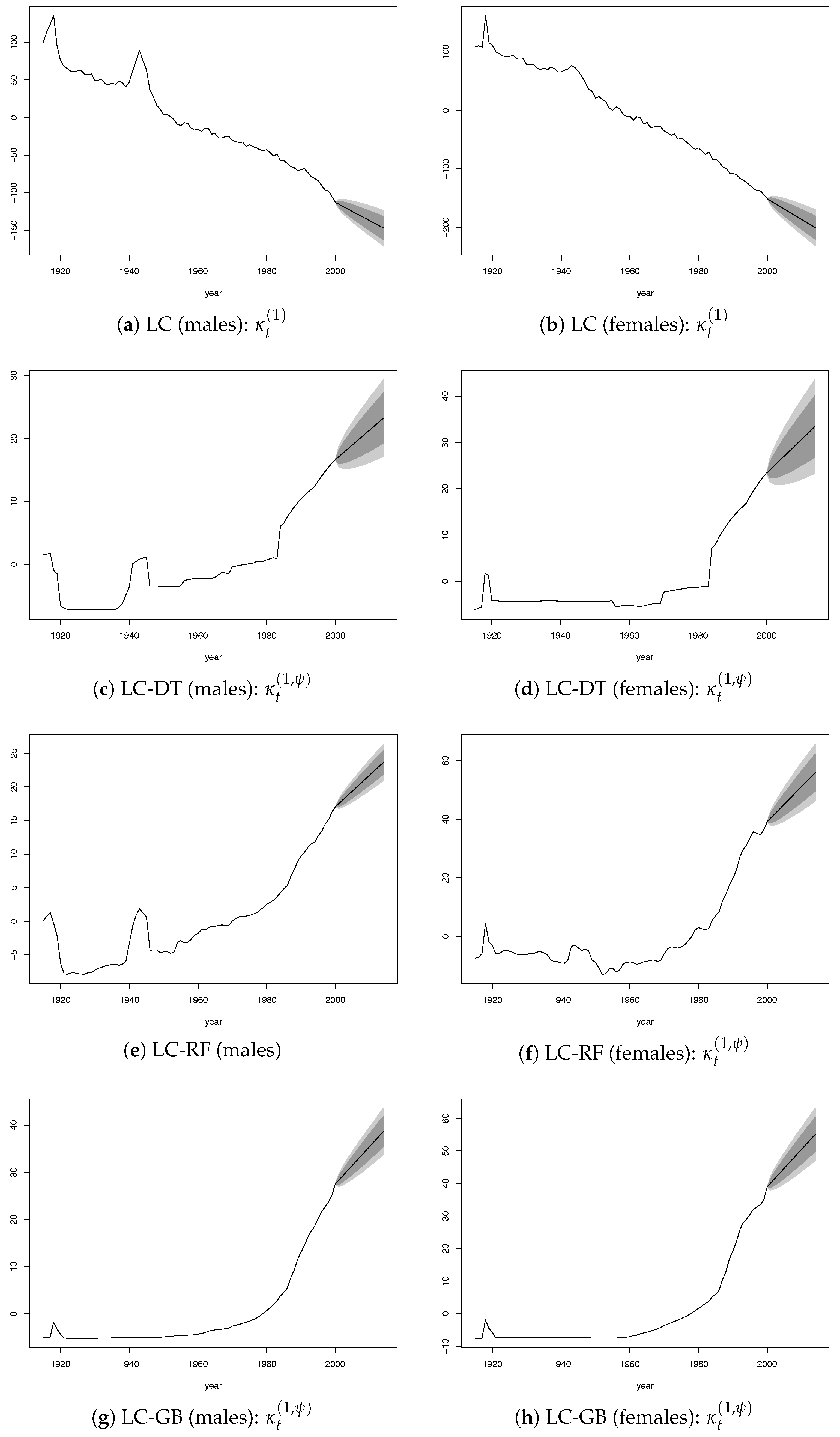
To verify the model accuracy, we provide out-of-sample forecasts, where the fitting period was set to 1915–2000 and the forecasting period to 2001–2014. In the forecasting, ${\kappa }_t^{(1,\psi )}$ and ${\kappa }_t^{(1)}$ were both modeled by a random walk with drift using values for the past 41 years (1960–2000). The plots of the time-dependent parameters ${\kappa }_t^{(1)}$ and ${\kappa }_t^{(1,\psi )}$ by gender are provided in the Appendix (Figure A2).

The values of parameter ${\kappa }_t^{(1)}$ of the LC standard model (Figure A2a,b) have been strongly decreasing from the end of the Second World War, which resulted in a strong reduction of mortality over time, with a further acceleration after the mid-1980s. The ML algorithms reduced this effect through the parameter ${\kappa }_t^{(1,\psi )}$,which showed a growing trend after 1960 with greater strength since the 1980s (Figure A2c–h).

The use of the same framework of the original mortality model to fit and forecast the ML estimators ${\widehat{\psi }}_{\mathbf{x}}$ has a dual purpose. On the one hand, it allows improving the forecasting provided by the original model and on the other hand analyzing the effect of the improvement directly on the model’s parameters. As discussed in the Introduction, machine learning is recognized to be very effective at detecting unknown and unidentifiable patterns in the data, but lacks an underlying theory that may be fundamental to provide a rational explanation of the results obtained. From this point of view, our approach can contribute to filling the gap between machine learning and theory combining a data-driven approach with a model-driven one.

Goodness of Forecasting

The forecasting results given by the out-of-sample test were compared using two measures: the root mean squared logarithmic error (RMSLE) and the root mean squared error (RMSE). The first one (RMSLE) takes into account $log{m}_{\mathbf{x}}$, providing a relatively large amount of weight to errors at young ages, while the second one (RMSE) is based on $m_{\mathbf{x}}$ and provides a relatively large amount of weight to errors at older ages.

$$\mathrm{RMSLE}=\sqrt{\frac{{\sum }_{\mathbf{x}}{\left(log({\widehat{m}}_{\mathbf{x}})-log(m_{\mathbf{x}}))\right)}^2}{N}}$$

(16)

$$\mathrm{RMSE}=\sqrt{\frac{{\sum }_{\mathbf{x}}{\left({\widehat{m}}_{\mathbf{x}}-m_{\mathbf{x}}\right)}^2}{N}}$$

(17)

Table 4. Out-of-sample test results: RMSLE and RMSE for the LC model without and with machine learning. ML estimator ${\widehat{\psi }}_{\mathbf{x}}^{\mathrm{LC},\mathrm{ML}}$ modeled according to the LC framework. Years 2000–2014 (fitting period: 1915–2000). Values in bold indicate the model with the smaller RMSLE and RMSE.

	RMSLE		RMSE
Model	Males	Females	Males	Females
LC	0.0290	0.0195	0.7282	0.7734
LC, DT	0.0139	0.0068	0.3567	0.5351
LC, RF	0.0083	0.0044	0.3624	0.1532
LC, GB	0.0100	0.0056	0.3536	0.1841

shows the out-of-sample test results for the LC model improved by machine learning when ${\widehat{\psi }}_{\mathbf{x}}^{\mathrm{LC},\mathrm{ML}}$ was forecasted using the LC framework. Values in bold indicate the model with the smaller RMSLE and RMSE. The RF algorithm provided the best performance, except for male RMSE, where GB was the best. The higher reduction of RMSLE was 77% for male and 71% for female, while when considering RMSE, it was 51% for male and 80% for females. However, we can conclude that all the ML estimators produced a significant improvement in forecasting with respect to the standard LC model.

4.4. Results for a Shorter Estimation Period: 1960–2014

We now use a more recent period (starting from 1960 instead of 1915) to analyze the level of the improvement provided by ML algorithms on a smaller dataset. The aim was to check if the change of the calibration period can have an important impact on the results, since the ML algorithms work better with larger datasets. We show in

Table 5. MAPE of fitted with respect to observed data for the LC, RH, and Plat model, before (No ML) and after (DT, RF, GB) the application of ML algorithms. Ages 0–100 and years 1960–2014, Italian population. Values in bold indicate the specification with the smaller MAPE for each model.

Gender	Males			Females
Model	LC	RH	Plat	LC	RH	Plat
No ML	11.08%	8.51%	12.67%	9.20%	8.44%	12.32%
DT	5.86%	5.27%	6.25%	5.90%	5.71%	6.62%
RF	4.07%	4.02%	3.89%	4.95%	4.79%	4.81%
GB	6.04%	4.84%	6.07%	5.49%	5.16%	6.27%

the values of MAPE used to analyze the quality of fitting. Furthermore, for a shorter calibration period, all the ML algorithms improved the standard stochastic mortality models, and the level of the improvement in the model fit remained high. The RF algorithm continued to be the best one.

The values of $\Delta m_{\mathbf{x}}^{\mathrm{mdl},\mathrm{ML}}$ for the LC, RH, and Plat model combined with the tree-based ML algorithms for the new calibration period are shown in Figure 5 for males. Similar results were obtained for females and are reported in the Appendix (see Figure A3).

Also in this case, there were significant changes, but there were less regions identified by diagonal splits (highlighting a cohort effect) with respect to the time period 1915–2014. Moreover, we observed that the significant changes were concentrated both in the young and old ages. The concentration in the old ages was less evident in the 1915–2014 analysis.

Out-of-sample tests were performed on the forecasting period 2001–2014, while the fitting period was set to 1960–2000. Also in this case, ${\kappa }_t^{(1,\psi )}$ and ${\kappa }_t^{(1)}$ were both modeled by a random walk with drift using values from 1960–2000. The plots of ${\kappa }_t^{(1)}$ and ${\kappa }_t^{(1,\psi )}$ by gender are provided in the Appendix (Figure A4). Different from the results obtained with the dataset for 1915–2000, where ${\kappa }_t^{(1,\psi )}$ showed a roughly monotone trend since 1960, in the case of a shorter estimation period, this trend oscillated: decreasing until the mid-1980s, increasing until 1997, then decreasing and increasing again for a few years (see Figure A2c–h and Figure A4c–h). As a consequence, the values of future ${\kappa }_t^{(1,\psi )}$ were approximately constant (due to the random walk with drift behavior), while they were increasing in the case of a longer estimation period (1915–2000). We observed that the reduction of mortality over the time period 1960–2000 was less strong than that registered for the years 1915–20002, and this fact led to more adequate projections, requiring less adjustments from ${\kappa }_t^{(1,\psi )}$.

Goodness of Forecasting

Table 6. Out-of-sample test results: RMSLE and RMSE for the LC model without and with machine learning. Years 2000–2014 (fitting period: 1960–2000). Values in bold indicate the model with the smaller RMSLE and RMSE.

	RMSLE		RMSE
Model	Males	Females	Males	Females
LC	0.0309	0.0183	0.3298	0.1840
LC, DT	0.0115	0.0074	0.3212	0.1789
LC, RF	0.0100	0.0066	0.3095	0.1761
LC, GB	0.0102	0.0070	0.3028	0.1730

shows the out-of-sample test results for the LC model. Values in bold indicate the model with the smaller RMSLE and RMSE. The best performance in terms of RMSLE was given by the RF algorithm, while in terms of RMSE, GB provided smaller values. The higher reduction of RMSLE was 68% for male and 64% for female, while in terms of RMSE, it was 8% for male and 6% for females.

In light of these results, we can state that, also with a smaller dataset, all the ML estimators produced a better quality of forecasting with respect to the standard LC, but the level of the improvement was less satisfactory for the older ages than the one obtained with the larger dataset (1915–2014). The reduction level obtained by RMSE for both genders was significantly lower than that achieved in the case of the 1915–2014 dataset. ML algorithms require large datasets to attain excellent performance, and using a smaller dataset makes the algorithms less effective in detecting unknown patterns, especially at old ages, where there are few observations.

5. Conclusions

Our paper illustrates how machine learning can be used to improve both fitting and forecasting of standard stochastic mortality models (such as LC, RH, and Plat), taking the advantages of artificial intelligence to better understand processes that are not identifiable by standard models. We extend the work of Deprez et al. (2017), which applied a regression tree boosting machine to improve the fitting of the LC and the RH model. We tested the improvement in the fitting quality of the LC, RH, and Plat model using not only the decision tree, but also two more powerful ML algorithms: random forest and gradient boosting. Our results, obtained from a case study structured on the Italian population, demonstrate that the random forest algorithm was more effective, though the other two algorithms produced significant improvements.

However, the main novelty of the proposed framework is the introduction of an ML estimator to improve the forecasting quality provided by standard stochastic models, where machine learning was used as a support and not as a substitute for them. Going away from the logic of machine learning, we forecasted the ML estimator using the same framework as the original mortality model. This idea was developed in the LC model framework. This approach aims to both improve the forecasted mortality rates provided by the standard LC and create a bridge between machine learning and theory to help find a rational explanation of the results. All the analysis was carried out on two different calibration periods: 1915–2014 and 1960–2014. Out-of-sample test results were encouraging, especially when considering the longer calibration period.

References

- Alpaydin, Ethem. 2010. Introduction to Machine Learning, 2nd ed. Cambridge: Massachusetts Institute of Technology Press, ISBN 026201243X. [Google Scholar]
- Breiman, Leo, Jerome Friedman, Richard Olshen, and Charles Stone. 1984. Classification and Regression Trees. Boca Raton: CRC Press, ISBN 9780412048418. [Google Scholar]
- Breiman, Leo. 2001. Random forests. Machine Learning 45: 5–32. [Google Scholar] [CrossRef]
- Brouhns, Natacha, Michel Denuit, and Jeroen K. Vermunt. 2002. A Poisson log-bilinear regression approach to the construction of projected lifetables. Insurance: Mathematics and Economics 31: 373–93. [Google Scholar] [CrossRef]
- Cairns, Andrew J. G., David Blake, Kevin Dowd, Guy D. Coughlan, David Epstein, Alen Ong, and Igor Balevich. 2009. A quantitative comparison of stochastic mortality models using data from England and Wales and the United States. North American Actuarial Journal 13: 1–35. [Google Scholar] [CrossRef]
- Deprez, Philippe, Pavel V. Shevchenko, and Mario V. Wüthrich. 2017. Machine learning techniques for mortality modeling. European Actuarial Journal 7: 337–52. [Google Scholar] [CrossRef]
- Haberman, Steven, and Arthur Renshaw. 2011. A comparative study of parametric mortality projection models. Insurance: Mathematics and Economics 48: 35–55. [Google Scholar] [CrossRef] [Green Version]
- Hainaut, Donatien. 2018. A neural-network analyzer for mortality forecast. Astin Bulletin 48: 481–508. [Google Scholar] [CrossRef]
- Hastie, Jerome, Trevor Hastie, and Robert Tibshirani. 2016. The Elements of Statistical Learning, 2nd ed. Data Mining, Inference, and Prediction. New York: Springer, ISBN 0387848576. [Google Scholar]
- Hunt, Andrew, and Andrés M. Villegas. 2015. Robustness and convergence in the Lee-Carter model with cohorts. Insurance: Mathematics and Economics 64: 186–202. [Google Scholar] [CrossRef]
- James, Gareth, Daniela Witten, Trevor Hastie, and Robert Tibshirani. 2017. An Introduction to Statistical Learning: With Applications in R. New York: Springer, ISBN 1461471370. [Google Scholar]
- Lee, Ronald D., and Lawrence R. Carter. 1992. Modeling and forecasting US mortality. Journal of the American Statistical Association 87: 659–71. [Google Scholar]
- Liaw, Andy. 2018. Package Randomforest. Available online: https://cran.r-project.org/ web/packages/randomForest/randomForest.pdf (accessed on 21 May 2018).
- Plat, Richard. 2009. On stochastic mortality modeling. Insurance: Mathematics and Economics 45: 393–404. [Google Scholar]
- Renshaw, Arthur E., and Steven Haberman. 2006. A Cohort-Based Extension to the Lee-Carter Model for Mortality Reduction Factors. Insurance: Mathematics and Economics 38: 556–70. [Google Scholar] [CrossRef]
- Richman, Ronald, and Mario V. Wüthrich. 2018. A Neural Network Extension of the Lee-Carter Model to Multiple Populations. Rochester: SSRN. [Google Scholar]
- Ridgeway, Greg. 2007. Generalized Boosted Models: A Guide to the gbm Package. Available online: https://cran.r-project.org/web/packages/gbm/gbm.pdf (accessed on 21 May 2018).
- Therneau, Terry M., and Elizabeth J. Atkinson. 2017. An Introduction to Recursive Partitioning Using the RPART Routines. Available online: https://cran.r-project. org/web/packages/rpart/vignettes/longintro.pdf (accessed on 21 May 2018).
- Villegas, Andrés M., Pietro Millossovich, and Vladimir K. Kaishev. 2015. Stmomo: An r Package for Stochastic Mortality Modelling. Available online: https://cran.r-project.org/web/packages/StMoMo/vignettes/StMoMoVignette.pdf (accessed on 21 May 2018).