Mortality Projections for Small Populations: An Application to the Maltese Elderly

Abstract

In small populations, mortality rates are characterized by a great volatility, the datasets are often available for a few years and suffer from missing data. Therefore, standard mortality models may produce high uncertain and biologically improbable projections. In this paper, we deal with the mortality projections of the Maltese population, a small country with less than 500,000 inhabitants, whose data on exposures and observed deaths suffers from all the typical problems of small populations. We concentrate our analysis on older adult mortality. Starting from some recent suggestions in the literature, we assume that the mortality of a small population can be modeled starting from the mortality of a bigger one (the reference population) adding a spread. The first part of the paper is dedicated to the choice of the reference population, then we test alternative mortality models. Finally, we verify the capacity of the proposed approach to reduce the volatility of the mortality projections. The results obtained show that the model is able to significantly reduce the uncertainty of projected mortality rates and to ensure their coherent and biologically reasonable evolution.

1. Introduction

Improving the accuracy of mortality projections is of great importance in actuarial science: in pricing, reserving and risk management of annuity business as well as in pensions and health care plans. In such activities, actuaries are often faced with the problem of modeling the mortality of small populations: e.g., small countries, a specific region of a country, an annuity portfolio and the participants of a pension or a health care plan. In the small populations, mortality rates are more affected by random fluctuations than in larger ones. Furthermore, the empirical records from small populations might only be available for relatively short periods and some data could be missing.

These features lead to difficulties in identifying the underlying trends. Due to these reasons, a model usually adopted for large populations could be inadequate for the smaller ones. Among others, Booth et al. (2006) have reported the limitations in the use of the Lee–Carter model on small populations. Moreover, as a result of the fact that data may only be available for short periods, mortality projections are rather uncertain. Forecasts are very sensitive to the fitting period and simple extrapolation of historic trends could produce “implausible projections and unrealistic age-profiles” (Jarner and Kryger (2011)).

Malta, with its small population, is undoubtedly an exemplary case. In accordance with the above, the development of its mortality rates shows great variability and irregular patterns and its data have more missing records than other countries; therefore, the use of standard mortality models may not be applicable and could lead to unreliable results.

Besides small populations, the focus of this work is on the older adult mortality. This represents an issue faced by many researchers in the field (e.g., Bongaarts (2005)). The Lee–Carter methodology tends to systematically under-predict the gains in old age mortality, due to the fact that, recently, old age improvements rates have gradually risen over time.

Regarding this issue, coherently with the Lee–Carter hypothesis of invariant improvement rates over time, one solution may be to adopt data related to shorter periods (see, among others, Booth et al. (2006)). As noted by Jarner and Kryger (2011), this approach allows us to overcome the problem of prediction, but, by restricting the observed period, its application seems to be limited.

For these reasons, we have focused our study only on this segment of the population, considering that infant and child mortality have quite a different nature from adult mortality. Furthermore, older adults are also the age-group of greatest interest in actuarial applications, such as pricing, reserving and risk management for life annuity portfolios or pension funds.

The literature on the subject of mortality modeling is very extensive but is mostly concerned with regular data. However, the issue of mortality in small populations has also been the subject of study and application of various methodologies. One way to deal with these problems could be the replication of the original data, which may lead to loss of specific information, or data smoothing using graduation methods (see Benjamin and Pollard (1993) and Bravo and Malta (2010)).

An example of the modeling of the mortality of small populations is the Saint model (Jarner and Kryger (2011)). It is based on observations of the Danish population, in which mortality rates vary considerably over time and for different ages, violating the Lee–Carter assumptions. The difficulty in obtaining plausible predictions with the classical models applied to small populations is related to the low number of exposures, to the high variability and to the high sensitivity with respect to the period under consideration.

It has been widely demonstrated that populations socially and economically similar could be modeled jointly, and this is very useful in the case of small populations, as one can overcome the disadvantages of limited data. This is why, when working on small demographic data, the most common idea is to borrow information from a larger and similar population. The use of a large population to improve the forecasts of the small one could be conducted:

• “by mixing appropriately the mortality data obtained from other populations” (e.g., Ahcan et al. (2014));
• by creating a two-population mortality model, which considers jointly the mortality of a small population related to a larger one.

Regarding multi-population mortality models, the most important contributions on this topic are:

• Li and Lee (2005), who applied the Lee–Carter model, with the introduction of common factors, for a group of given population, in order to predict single mortality evolution;
• Cairns et al. (2011a), who introduced a Bayesian framework to jointly model two populations, referring to one of them as sub-population of the other one;
• Dowd et al. (2011), who proposed the gravity model for two populations in order to obtain coherent mortality forecasts;
• Jarner and Kryger (2011), who proposed a model for the Danish mortality (the Spread Adjusted InterNational Trend (SAINT) model) combining the mortality deterministic evolution of a basket of population with the stochastic evolution of the spread;
• D’Amato et al. (2014), who extended the Lee–Carter model in order to take into account the existence of dependence in mortality data across multiple populations;
• Villegas and Haberman (2014), who applied a relative modeling approach where the death rates of a subpopulation are modeled in relation to the death rates of a reference population; they considered different multiple population extensions of the Lee–Carter model and applied their approach in order to study and forecast socioeconomic mortality differentials across deprivation subgroups in England;
• Kleinov (2015), who developed a common age affect variants of the Lee–Carter model with p age and period factors for modeling the mortality of multiple populations;
• Li et al. (2015), who generalize a single-population mortality model in different possible ways, in order to fit two or more populations and to measure the basis risk in longevity hedges;
• Wan and Bertschi (2015), who proposed a two part model to fit Swiss historical data and make coherent forecasts, taking information from a larger population;
• Antonio et al. (2017), who developed a Li and Lee multi-population model to project Dutch and Belgian mortality evolution and measure the actuarial implication of their model;
• Chen et al. (2017), who proposed “the use of parametric bootstrap methods to investigate the finite sample distribution of the maximum likelihood estimator for the parameter vector of a stochastic mortality model”;
• Hunt and Blake (2017), who modeled the mortality rates of a pension scheme through an Age Period Cohort (APC) model that has the same form of the reference population model but is characterized by scaling factors that multiply period and cohort parameters and reduce or increase the dependence between the two models;
• Villegas et al. (2017), who developed a comprehensive comparative study of mortality models for two populations proposed in the literature and applied them to the case of a population of a pension scheme in order to measure the basis risk involved in longevity hedges;
• Wang et al. (2018), who proposed an approach based on a combination of data aggregation and mortality graduation applied to the empirical data from Taiwan and Taipei City.

We follow the approaches of Jarner and Kryger (2011) and Wan and Bertschi (2015). In both works, a two-step routine has been used, consisting of a first phase in which the mortality of a reference population is modeled; it is followed by the estimation of the parameters of the mortality spread between the two populations. The Jarner and Kryger model is based on the hypothesis that in the small population mortality evolves around a smooth surface (the trend, whose parameters are estimated in a frailty model). The deviation from this surface is the spread and it is modeled by regressors referring to the age-profiles and the evolution over time of its components. In particular, they propose three age-profile regressors to capture level, slope and curvature of the deviation between the reference surface and the specific small population mortality. Wan and Bertschi use a Plat model and a Lee–Carter (with m time factors) to model the reference part and the spread, respectively. In both of these works, the reference population is a basket of populations worldwide that include the population of interest; unlike their proposal, in our paper, the choice of the reference population does not fall in a basket of populations. Similarly to Ahcan et al. (2014), we believe that the procedure is more effective by adopting as a reference population a population close (geographically, historically or socio-economically) to the small population to be modeled (in our case the Maltese one). We use, as reference, one country population and the first step of the analysis consists of determining the population to be taken as a reference on a set of possible candidates. Once the reference population has been chosen, we construct a two-part mortality model in order to describe the evolution of the small population: the first component is the trend, the second component is the spread.

Unlike the two works mentioned above, in this paper, the choice of the models to be used for the two populations takes place through a two-stage selection procedure: first, we identify the mortality models that most suitably represent the mortality of the reference population, then we choose the model for the spread through an analysis of all the possible mix of considered models, as well as the results of the previous stage.

The rest of this paper is organized as follows: in Section 2, we analyze the possible reference populations and choose the best one; in Section 3, we choose the mortality models for the reference population and the Maltese one; Section 4 contains the forecasts obtained from the application of the models; in Section 5, some final conclusions are deduced.

2. The Model Structure and the Choice of the Reference Population

2.1. The Model Structure

The goal of this study is to overcome the problems related to the small size of the mortality data for a small population. In particular, the purpose is to take information about the trend from the mortality dynamics of another population assumed as the reference one, which has the following characteristics:

• being greater than the one for which we want to predict mortality;
• having a background trend similar to that of the smaller population’s mortality.

We denote by $d_{x,t,i}$, and by $E_{x,t,i}$, respectively, the number of deaths and the exposure in the population i, at age x in the year t. Data refer to k ages, $x\in [x_1,x_k]$, and n calendar years, $t\in [t_1,t_n]$. The central death rate is given by:

$$m_{x,t,i}=d_{x,t,i}/E_{x,t,i}.$$

(1)

We assume that the number of deaths follow a Poisson distribution:

$$d_{x,t,i}\sim Poisson\left(E_{x,t,i}{m}_{x,t,i}\right).$$

(2)

The spread between the mortality of the small population, s, and the reference one, r, is modeled as follows:

$$m_{x,t,s}={\widehat{m}}_{x,t,r}{S}_{x,t},$$

(3)

where ${\widehat{m}}_{x,t,r}$ are the fitted values of death rates for the reference population and $S_{x,t}$ the spread between the death rates of the two populations. Under these assumptions, the first step is to choose the reference population.

The methodologies for this choice are neither unique nor simple and have to be relativized according to the research and characteristics of the available data. There should be similarities in the shape of mortality rates of small population and that of the reference one. Moreover, there should be no differences in trend between the selected reference population and the small one. In the literature, several useful indices were presented in order to measure similarities and differences of mortality between different populations. Keyfitz and Caswell (2005), for example, have shown different approaches to the study of similarities between phenomena in different populations and over time. The use of direct and indirect standardization is very common when the populations in comparison are different in terms of the structure and scale of dataset records.

We have considered four different countries as candidates for the reference population: France, Italy, Spain and United Kingdom. These countries have similar patterns of demographic transitions. Malta started its demographic transition later, but completed it within a relatively short period of one generation. By the end of the 1970s, the birth and mortality rates fell to the same levels as other European countries that had completed their demographic transitions many years before.

Among these four countries, the United Kingdom is historically and culturally close to Malta, which was a British colony from 1814 (Congress of Vienna) until the independence declaration (21 September 1964). France, Italy and Spain were also evaluated according to a geographical criterion, considering that Italy is the closest to Malta and the other two border the Mediterranean Sea. Other Mediterranean countries were excluded from the analysis due to the socio-political divergences that inevitably differentiate them from Malta as regards mortality levels (for example North-African countries and Turkey) or due to lack of data (for example, Greece, for which data about the number of deaths are available on the Human Mortality Database until 2013).

2.2. Mortality Data

In order to select the reference population and build the model, for each of the considered populations, we have used the historical mortality dataset composed of the number of deaths and central exposures by age and year, from 1999 up to 2016 and for the ages 60–89. For a short overview of Malta’s demographic situation, we report that the number of Maltese exposures of all ages in 2016 was equal to 437,479, while the number of exposures for the age range 60–89 was equal to 58,959 females and 51,438 males. Considering that mortality data of Malta are not available in the Human Mortality Database (while Eurostat provides data starting from year 2006), we can not use the same data source for all the countries involved in the analysis. A part of mortality data of Malta (data about the period from 2001 to 2014) is published online by the National Statistics Office of Malta, but the whole dataset has been obtained thanks to the Population and Migration Unit of the National Statistics Office (NSO) of Malta. The deaths in this dataset represent the current values registered in the country, analysed by the Health Information and forwarded to the NSO. Data concerning the mid-year population aged x in the year t are obtained as the average of the populations at the end of each year. These data are about the total population in Malta (in this section, we denote “total population” that includes both Maltese and foreign residents). The population on 31 December 1998 and 1999 by age was provided only for the Maltese population, $M_{pop}(x,t)$ (we consider only “Maltese born population”, excluding permanent foreign residents). However, total population of all ages, $T_{pop}\left(t\right)$, on 31 December 1998 and 1999 were provided. In order to use consistent data for the entire time period, the estimates of total population on 31 December 1998 and 1999 by age, $T_{pop}(x,t)$, are obtained based on the available data, by applying the following formula:

$$T_{pop}(x,t)=\frac{M_{pop}(x,t)}{M_{pop}\left(t\right)}{T}_{pop}\left(t\right),$$

(4)

where $M_{pop}\left(t\right)={\sum }_x{M}_{pop}(x,t)$, $t=\mathrm{31.12.1998}, \mathrm{31.12.1999}$ and $x=0,\dots ,\omega$, with $\omega$ denoting the extreme age. This formula has been applied both for female and male populations. For other countries, data are available on the Human Mortality Database (HMD) (HMD (2018)), except for data about Italy in the years 2015–20161, which are obtained from the ISTAT (National Institute of Statistics) (ISTAT (2015), ISTAT (2016)). As documented in the “Data sources” section of the HMD website, the data about Italy available in the Human Mortality Database are provided by ISTAT, therefore the two data sources are aligned. Specifically, for 2015 and 2016, the values of mid-year population by age are obtained from those of the population at the beginning of the years (published on the ISTAT website). As regards the number of deaths in 2015 and 2016, deaths by age are not available on the ISTAT website, so they have been obtained through a two-step procedure:

• firstly, the mortality rates derived from the death probabilities2;
• then, from these values and those of mid-year population, number of deaths are easily calculated.

In order to check the reliability of this procedure, we have taken data from ISTAT in a randomly chosen previous year and estimate in the same way the number of deaths by age and year. Comparing the values obtained to those available on the HMD, we find out that almost all the percentage variations are negligible.

2.3. The Choice of the Reference Population

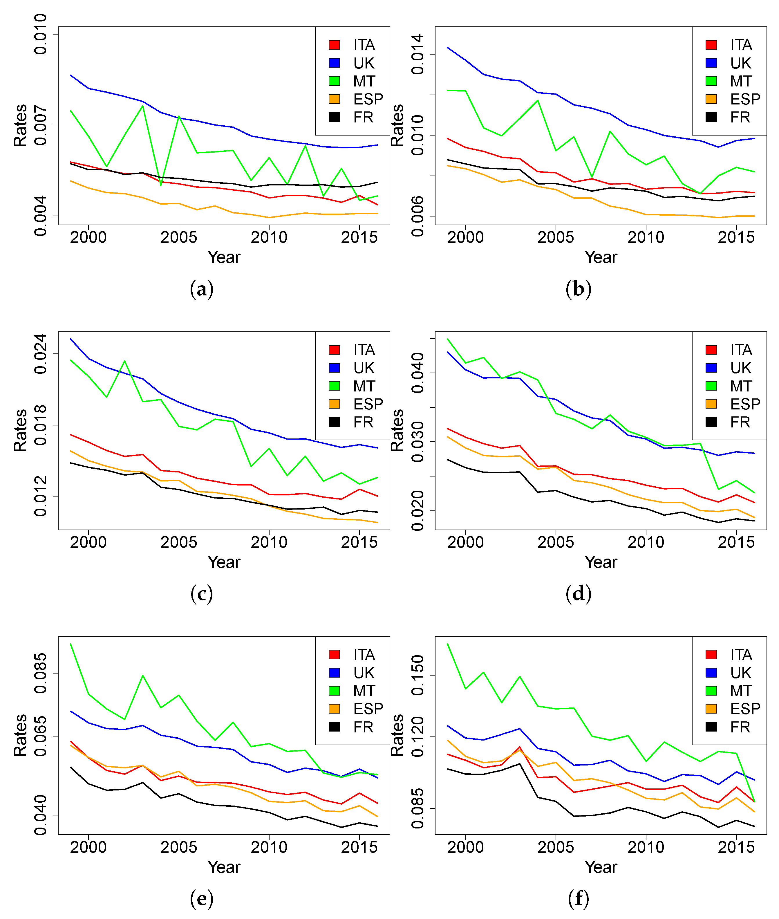
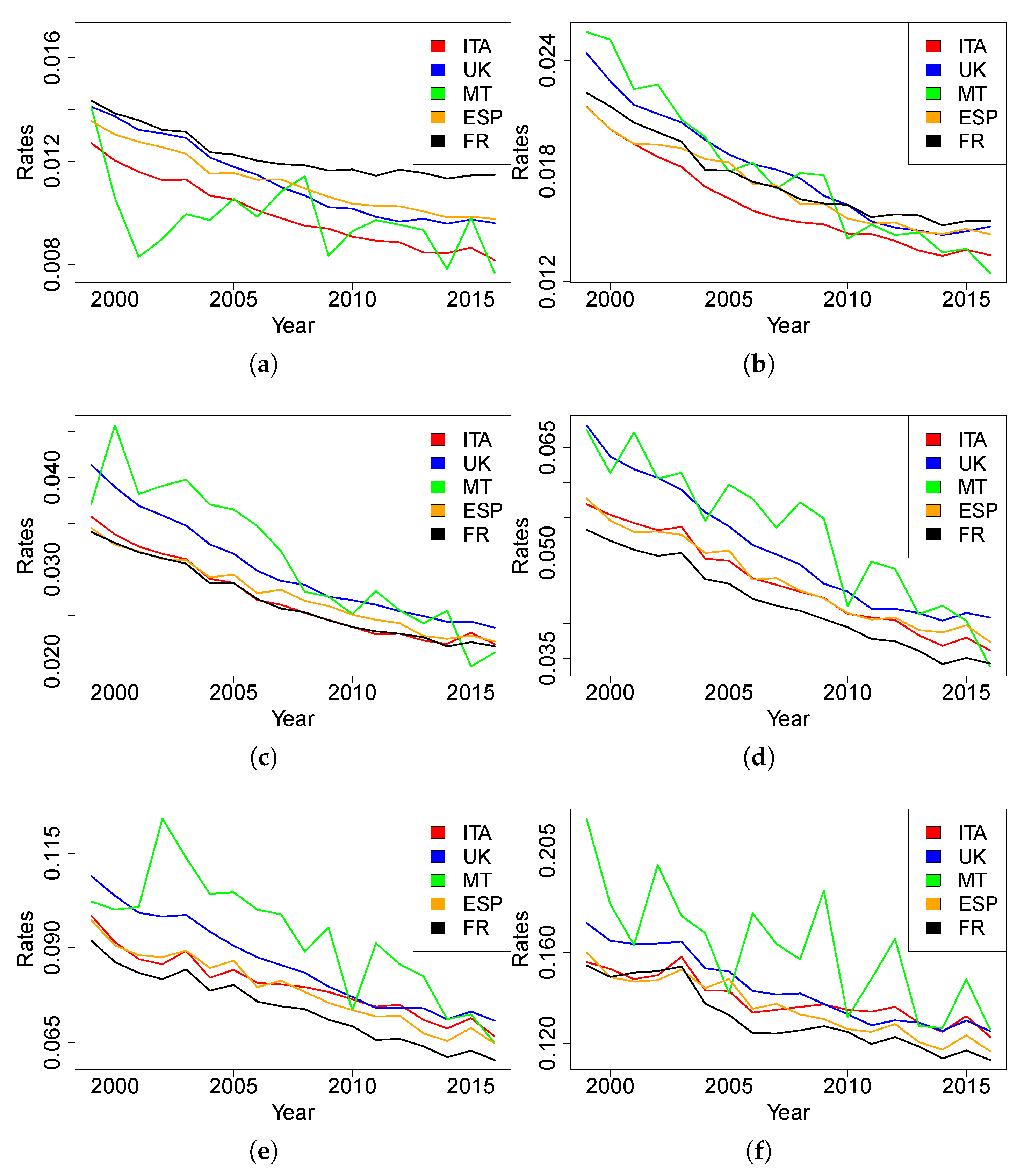
In this section, we report different indices, calculated by comparing the mortality of Malta with the mortality of the four countries candidates to be the reference population; the indices are calculated for both genders. It might be worth to plotting the evolution of the death rates referred to five-year age ranges (Figure 1 and Figure 2 for females and males, respectively).

As expected, the age(-range)-specific death rates of Malta over time are much less stable than other countries. This is attributable to the scale of the available data, which generates more random fluctuations than is the case of bigger populations. In this case, because of rate variability, we cannot gather evidence on which trend is closer to the Maltese one.

The comparison between the countries is affected by the different population sizes and mostly by the different age structures. In order to have a more realistic comparison, a common method is to use standardization procedures. We use a direct standardization in which the standard age structure is provided by a standard population. Considering that the purpose here is to compare the mortality of different countries to that of Malta, we decided to assume Malta as a standard population. The Standardized Death Rates over time are plotted below, defined as:

$$SD{R}_{t,i}=\frac{{\sum }_{x=60}^{89}{E}_{x,t,s}{m}_{x,t,i}}{{\sum }_{x=60}^{89}{E}_{x,t,s}},$$

(5)

where $i=$ France, Italy, Malta, Spain and UK, $s=$ standard population (Malta) and $t=$1999,...,2016. This SDR allows us to eliminate the differences attributable to the different dimensions and structures of the populations. Once the effect of the structure is removed, the values are comparable and give a measure of closeness or distance of mortality in the countries considered. From Figure 3, we can observe that the general trend and the slight decrease of values over time of the Maltese mortality seem to be closer to the dynamics of UK mortality than those of other countries.

Additionally, we can calculate a Relative Measure of Mortality (RM), by dividing the SDRs of France, Italy, Spain and UK by the crude death rates of Malta, obtaining the following formula:

$$R{M}_{t,i}=\frac{{\sum }_{x=60}^{89}{E}_{x,t,s}{m}_{x,t,i}}{{\sum }_{x=60}^{89}{E}_{x,t,s}{m}_{x,t,s}},$$

(6)

where $i=$ France, Italy, Spain and UK, $s=$ standard population (Malta) and $t=$ 1999, …, 2016. Over time, the more the RM index for a country has a value near to 1, the closer its mortality is to Malta’s mortality. From Figure 4, we can observe that the values of RM of France, Italy and Spain are systematically under 1 (and under those of UK), showing that their mortality is lower than that of Malta in each year, except for male mortality in 2010 and 2016. The results obtained with this additional measure suggest that United Kingdom may be suitable as a reference to model the mortality of Malta. In order to have quantitative support on the selection of the reference population, further analysis follows in the next section.

2.4. An Alternative Approach for the Choice of the Reference Population

In defining the reference population, an alternative approach could be to mix data from different countries as in Ahcan et al. (2014). In particular, they proposed to mitigate the fluctuations in the mortality profile of a small population (the Slovenian one) preserving its own features, replacing the mortality rates of the small population with the weighted averages of neighboring countries mortality data. This approach is based on the minimization of the sum of the (squared) differences between the observed age-specific mortality rates of the small population with the weighted averages of different countries age-specific mortality rates. We have applied this method to the observed Maltese mortality rates and the weighted averages of the mortality rates of the four populations considered as possible reference: France, Italy, Spain and United Kingdom. The optimization problem is defined as follows:

$$\begin{array}{c}\underset{w_i}{\min }\sum _{t=1999}^{2016}\sum _{x=60}^{89}{(m_{x,t,s}-m_{x,t,AVE})}^{2}i=1,\dots ,4,\hfill \\ \mathrm{s}.\mathrm{t}.\hfill \\ w_i\ge 0,\hfill \\ \sum _{i=1}^4{w}_i=1,\hfill \end{array}$$

(7)

where

$$m_{x,t,AVE}=\sum _{i=1}^4{w}_i{m}_{x,t,i}$$

(8)

and we refer to France for the population 1, Italy for the population 2, Spain for population 3 and, finally, to United Kingdom for the population 4 while population s is, as usual, the Maltese one. From this optimization procedure, we find that the weight of the British component in the optimum basket mortality data is over 0.99 while the weights for France, Italy and Spain all together sum for the remaining part.

This result confirms that the United Kingdom is the best candidate as reference population and that it would not be useful to consider a basket of countries considering that the weight of the remaining countries would be substantially insignificant.

For all these reasons, in the following, we have decided to use UK mortality data as reference in the estimation of Maltese mortality.

3. The Mortality Models Choice

Once the reference population used to “borrow” information on the general trend of the mortality profile of the small population has been chosen, the next step concerns the choice of mortality models for the reference population and the models for the spread. In order to do this, we followed a two-step procedure: first, we identified the model that best fits the observed mortality data of the reference population; then, we chose the spread model by analyzing the possible combinations between the models under consideration.

3.1. The Reference Population Mortality Model

In order to choose the model for the reference population, we fit UK mortality data, separately for each sex, LC (Lee and Carter (1992)), APC (Currie (2006)), RH (Renshaw and Haberman (2006)) and Plat models (Plat (2009)) respectively defined as (

Table 1. Mortality models for the reference population.

Model	Formula
LC	$log\left(m_{x,t,r}\right)={\alpha }_x^{\left(r\right)}+{\beta }_x^{(1,r)}{\kappa }_t^{(1,r)}$
APC	$log\left(m_{x,t,r}\right)={\alpha }_x^{\left(r\right)}+{\kappa }_t^{(1,r)}+{\gamma }_{t-x}^{\left(r\right)}$
RH	$log\left(m_{x,t,r}\right)={\alpha }_x^{\left(r\right)}+{\beta }_x^{(1,r)}{\kappa }_t^{(1,r)}+{\beta }_x^{(0,r)}{\gamma }_{t-x}^{\left(r\right)}$
Plat	$log\left(m_{x,t,r}\right)={\alpha }_x^{\left(r\right)}+{\kappa }_t^{(1,r)}+(\overline{x}-x){\kappa }_t^{(2,r)}+{\gamma }_{t-x}^{\left(r\right)}$

):

where ${\alpha }_x^{\left(r\right)}$ represents the mortality level at age x for the r population; the time processes ${\kappa }_t^{(1,r)}$ (for $i=1,2$) are the mortality trend for the population r while ${\beta }_x^{(1,r)}$ measures the sensitivity of mortality at age x to the respective time trend. ${\gamma }_{t-x}^{\left(r\right)}$ take in to account the cohort effect (if present) for the cohort born in year $t-x$ and ${\beta }_x^{(0,r)}$ measures the sensitivity of mortality at age x to the cohort effect.

Two different versions of the Renshaw–Haberman model could be considered: a simplified version in which we assumed ${\beta }_x^{\left(0\right)}$ equal to 1 for all ages and the standard one with non-parametric ${\beta }_x^{\left(0\right)}$. It is well known in the literature (see e.g., Haberman and Renshaw (2011) and Hunt and Villegas (2015)) that the Renshaw–Haberman model presents convergence issues which the simplified version addresses but does not completely eliminate. For this reason, in the following, we decided to consider the version of the Renshaw–Haberman model with ${\beta }_x^{\left(0\right)}$ equal to 1. The Plat model is used in its reduced form, i.e., we exclude the third temporal factor that refers to lower ages (that are not included in the data used).

The models are fitted with the R-package “StMoMo” (Villegas et al. (2018)). In order to ensure the identifiability of the parameters, the usual constraints adopted in the literature are used (see Cairns et al. (2009) and Plat (2009)). For the Renshaw–Haberman model, we impose the additional constraint proposed by Hunt and Villegas (2015) in order to make it more stable and faster to converge.

Table 2. Parameter constraints for the reference population model.

Model	Constraints
LC	${\sum }_x{\beta }_x^{(1,r)}=1$, ${\sum }_t{\kappa }_t^{(1,r)}=0$
APC	${\sum }_t{\kappa }_t^{(1,r)}=0$, ${\sum }_{t-x}{\gamma }_{t-x}^{\left(r\right)}=0$, ${\sum }_{t-x}(t-x){\gamma }_{t-x}^{\left(r\right)}=0$
RH	${\sum }_x{\beta }_x^{(1,r)}=1$, ${\sum }_t{\kappa }_t^{(1,r)}=0$, ${\sum }_{t-x}{\gamma }_{t-x}^{\left(r\right)}=0$, ${\sum }_{t-x}(t-x-(\overline{t}-\overline{x})){\gamma }_{t-x}^{\left(r\right)}=0$
Plat	${\sum }_t{\kappa }_t^{(1,r)}=0$, ${\sum }_t{\kappa }_t^{(2,r)}=0$, ${\sum }_{t-x}{\gamma }_{t-x}^{\left(r\right)}=0$, ${\sum }_{t-x}(t-x){\gamma }_{t-x}^{\left(r\right)}=0$, ${\sum }_{t-x}{(t-x)}^2{\gamma }_{t-x}^{\left(r\right)}=0$

shows the parameter constraints imposed to the models.

In the fitting procedure, we have excluded the cohorts with less than four observations. The result of the models fitting in terms of log-likelihood, Akaike Information Criterion (AIC) and Bayesian Information Criterion (BIC)3 are reported in the following tables (In

Table 3. Models comparison for UK females.

	LogLik	AIC	BIC
LC	−3526.20(4)	7204.40(4)	7527.69(4)
APC	−3062.91(3)	6293.81(3)	6651.13(3)
RH	−2947.52(1)	6121.03(2)	6601.71(2)
Plat	−2955.81(2)	6111.62(1)	6537.00(1)

and

Table 4. Model comparison for UK males.

	LogLik	AIC	BIC
LC	−3505.45(4)	7162.90(4)	7486.20(4)
APC	−3132.11(3)	6432.22(3)	6789.54(3)
RH	−3017.30 (1)	6260.61(2)	6741.29(2)
Plat	−3029.96 (2)	6259.93(1)	6685.31(1)

for female and male, respectively) specifying in the brackets the ranking across models.

The results show that the RH model is always the best one in terms of log likelihood, but it is penalized by the greater number of free parameters when AIC or BIC criteria are considered. Adopting the AIC or BIC as choice criterion, the Plat model is the best one for both female and male population, while the second one is always the RH model. The LC model is the worst for all the criteria considered.

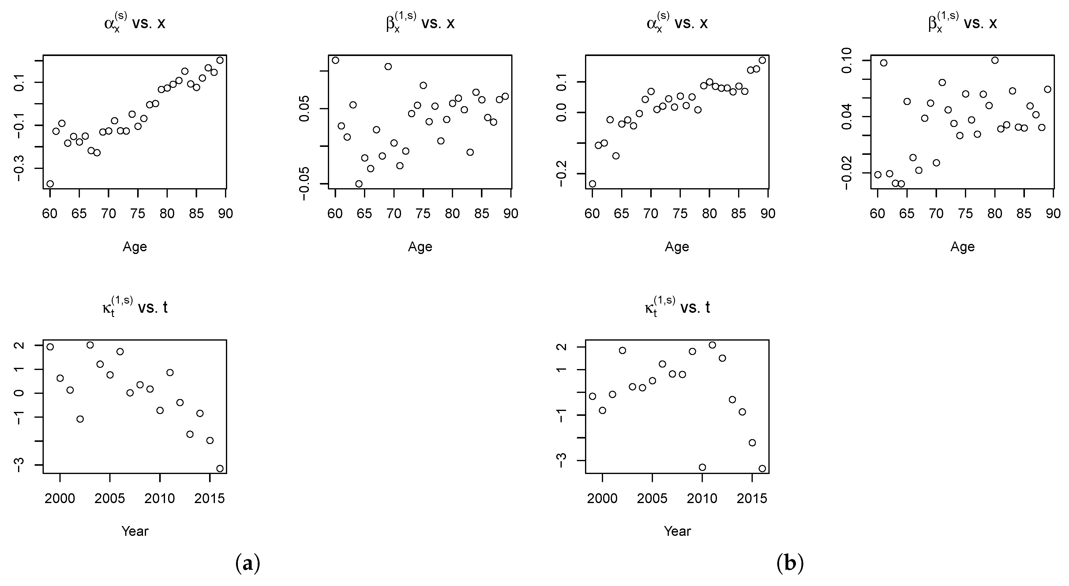
In view of these results, in the following, we consider the PLAT and RH models to represent the evolution of mortality in the reference population. In Figure 5, we report the fitted parameters of the RH model for the reference population.

As expected, the ${\alpha }_x^{\left(r\right)}$ term increases with age, whereas the mortality decreases over time, as shown by ${\kappa }_t^{(1,r)}$ estimations. The mortality decrease is higher at older ages as shown by the evolution of ${\beta }_x^{(1,r)}$. The ${\gamma }_{t-x}^{\left(r\right)}$ factor profiles are coherent with the expectations and literature findings on cohort effect (see the work of Willets (2004), but also Renshaw and Haberman (2006), Cairns et al. (2009) and Haberman and Renshaw (2011)): it increases until the end of the 1920s and then decreases.

The fitted parameters of the Plat model are reported in Figure 6.

Also in the Plat model case, the ${\alpha }_x^{\left(r\right)}$ term is coherently increasing with age, the mortality is decreasing over time, as shown by ${\kappa }_t^{(1,r)}$ estimations. With reference to the cohort effect, ${\gamma }_{t-x}^{\left(r\right)}$, we observe a similar pattern with respect to the values obtained with the RH model, unless the last cohorts (born after 1945).

3.2. The Model Choice for the Spread

The final step of the approach proposed in this paper is the choice of the model for the spread (the ratio between the observed Maltese mortality rates and the fitted values of the British death rates) and the estimation of its parameters. Considering s the index for the small (Maltese) population, we assume the spread could be modeled by means of the same models previously considered for the reference population: Lee–Carter, Age Period Cohort, Renshaw–Haberman and Plat, then the spread is respectively defined as follows (

Table 5. Mortality models for the Spread.

Model	Formula
LC	$log\left(m_{x,t,s}\right)-log\left({\widehat{m}}_{x,t,r}\right)={\alpha }_x^{\left(s\right)}+{\beta }_{x,i}^{(1,s)}{\kappa }_t^{(1,s)}$
APC	$log\left(m_{x,t,s}\right)-log\left({\widehat{m}}_{x,t,r}\right)={\alpha }_x^{\left(s\right)}+{\kappa }_t^{(1,s)}+{\gamma }_{t-x}^{\left(s\right)}$
RH	$log\left(m_{x,t,s}\right)-log\left({\widehat{m}}_{x,t,r}\right)={\alpha }_x^{\left(s\right)}+{\beta }_x^{(1,s)}{\kappa }_t^{(1,s)}+{\gamma }_{t-x}^{\left(s\right)}$
Plat	$log\left(m_{x,t,s}\right)-log\left({\widehat{m}}_{x,t,r}\right)={\alpha }_x^{\left(s\right)}+{\kappa }_t^{(1,s)}+(\overline{x}-x){\kappa }_t^{(2,s)}+{\gamma }_{t-x}^{\left(s\right)}$

).

where ${\widehat{m}}_{x,t,r}$ are the fitted values of death rates for the reference population. In order to ensure the identifiability of the parameters, we adopt for the spread the same constraints adopted for the reference population. The results of the fit in terms of log-likelihood, AIC and BIC are reported in the following tables (in

Table 6. Models comparison for the female Maltese population.

LogLik
	Spread model
Trend model	LC	APC	RH	Plat
LC	−1591.82	−1592.24	−1576.74	−1586.54
APC	−1592.67	−1592.42	−1577.22	−1585.77
RH	−1592.87	−1593.39	−1577.69	−1586.09
Plat	−1592.17	−1592.76	−1577.18	−1585.77
AIC
	Spread model
Trend model	LC	APC	RH	Plat
LC	3335.64	3352.48	3379.47	3373.07
APC	3337.34	3352.85	3380.44	3371.54
RH	3337.74	3354.78	3381.38	3372.17
Plat	3336.34	3353.51	3380.36	3371.54
BIC
	Spread model
Trend model	LC	APC	RH	Plat
LC	3658.93	3709.80	3860.16	3798.45
APC	3660.63	3710.17	3861.12	3796.92
RH	3661.03	3712.10	3862.06	3797.56
Plat	3659.64	3710.83	3861.05	3796.92

and

Table 7. Models comparison for the male Maltese population.

LogLik
	Spread model
Trend model	LC	APC	RH	Plat
LC	−1661.38	−1653.98	−1634.86	−1639.59
APC	−1664.95	−1652.46	−1634.75	−1638.62
RH	−1663.67	−1652.29	−1633.15	−1638.54
Plat	−1663.33	−1651.21	−1632.79	−1638.62
AIC
	Spread model
Trend model	LC	APC	RH	Plat
LC	3474.77	3475.97	3495.72	3479.17
APC	3481.89	3472.92	3495.50	3477.24
RH	3479.34	3472.58	3492.31	3477.09
Plat	3478.67	3470.43	3491.59	3477.24
BIC
	Spread model
Trend model	LC	APC	RH	Plat
LC	3798.06	3833.29	3976.40	3904.56
APC	3805.18	3830.24	3976.19	3902.62
RH	3802.63	3829.91	3972.99	3902.47
Plat	3801.96	3827.75	3972.27	3902.62

for female and male, respectively).

Although in the previous step we observed that the best models for the reference population mortality were the Plat and the RH, for completeness in the following tables the values obtained from all the possible combinations of models have been reported: 16 combinations obtained as the product between the 4 models for the reference population and 4 models for the small population.

For both the female and male population, the best log-likelihood results are obtained when the spread is modeled with the RH model. Otherwise, when we consider the BIC, the best model for the spread is the LC one. Finally, considering the AIC, the LC model is preferable to model the spread for the female population while the APC is better for the male. Furthermore, we observe that the results are not very different when we change the model adopted for the reference population. As a consequence, the choice for the spread model can be made independently of the choice of the reference population model. Finally, from the results obtained, we can conclude that is not necessary to model a cohort effect for the spread separately. This aspect is desirable. Actually, Villegas et al. (2017) demonstrate the instability of the results obtained when a cohort term specific to the small population is included in the model. Considering the results obtained in the reference population model and in the spread model selection, we conclude that the best combinations to represent Maltese mortality are given by the RH–LC and the Plat–LC models. The final model for the RH–LC combination is defined as:

$$log\left(m_{x,t,s}\right)={\alpha }_x^{\left(r\right)}+{\beta }_x^{(1,r)}{\kappa }_t^{(1,r)}+{\gamma }_{t-x}^{\left(r\right)}+{\alpha }_x^{\left(s\right)}+{\beta }_x^{(1,s)}{\kappa }_t^{(1,s)}.$$

(9)

Meanwhile, the final model for the Plat–LC combination is defined as:

$$log\left(m_{x,t,s}\right)={\alpha }_x^{\left(r\right)}+{\kappa }_t^{(1,r)}+(\overline{x}-x){\kappa }_t^{(2,r)}+{\gamma }_{t-x}^{\left(r\right)}+{\alpha }_x^{\left(s\right)}+{\beta }_x^{(1,s)}{\kappa }_t^{(1,s)}.$$

(10)

Figure 7 shows the estimated parameters for the spread components for the RH–LC model.

Looking at the estimated age effects, Maltese mortality appears higher than in UK for older population (${\alpha }_x^{\left(s\right)}>0$); instead, for the younger population, the mortality is higher in UK (${\alpha }_x^{\left(s\right)}<0$). On the contrary, the temporal dynamics reveal higher mortality for Maltese women and men in the first years under consideration, since ${\kappa }_t^{(1,s)}>0$ for most of the years from 1999 to 2011, while it is smaller than zero in the last years.

Figure 8 shows the estimated parameters for the spread components for the Plat–LC model.

The parameter evolution of the spread component of the model is almost the same as that observed in the previous case. The residuals of the fitted model are used to investigate the goodness-of-fit of mortality models. In fact, when there is regularity in the residuals, the model is unable to describe all the characteristics of the data properly. Assuming a random Poisson component, it is useful to examine the scaled deviance residuals.

We provide plots of scaled deviance residuals between the observed and fitted number of Maltese deaths after application of both RH–LC and Plat–LC models. As shown in Figure 9, Figure 10, Figure 11 and Figure 12, the residuals have a symmetric and random disposition around 0, without presenting traces of paths not picked up by the fitted model.

The comparison of the models is then concluded by calculating, for both, the mean absolute percentage error (MAPE) defined as:

$$MAPE=\frac{1}{n}\sum _{t=1999}^{2016}\sum _{x=60}^{89}\left|\frac{m_{x,t,i}-{\widehat{m}}_{x,t,i}}{m_{x,t,i}}\right|\ast 100.$$

(11)

MAPE is then defined as the average absolute percent error for each period of the estimated death rates minus the actuals divided by actuals. MAPE is usually adopted as a measure of forecast error, for example in backtesting analysis (out of sample). Here, it is used as an in-sample goodness of fit measure.

From results reported in

Table 8. MAPE of the models for Maltese population.

	Females	Males
RH-LC	13.55%	12.82%
Plat–LC	13.50%	12.81%

, the Plat–LC model seems to fit the mortality data of Malta better than the RH–LC one, although the obtained results are very similar.

4. Mortality Projections

4.1. Time Series Dynamics

Mortality projections can be obtained once the dynamics of each period and the cohort parameter has been defined. With reference to the trend, even if other solutions can be explored, the time processes are usually modeled as random walk with drift in the models with only one period effect (as in the RH model) and as a multivariate random walk with drift for models with more than one period effects (as in the Plat model) (see Cairns et al. (2011b) and Villegas et al. (2017)). In

Table 9. BIC for different ARIMA processes for period effect in the RH model for the reference population.

		Females		Males
Process	d Order	Best ARIMA	BIC	Best ARIMA	BIC
${\kappa }_t^{(1,r)}$	d = 2	(0,2,1)	44.79	(0,2,1)	35.75
	d = 1	(0,1,0)	44.74	(0,1,0)	38.39
	d = 0	(3,0,0)	60.45	(3,0,0)	51.96

, we examine different ARIMA(p; d; q) processes for the period effect in the RH model for the reference population, with d = 0; 1; 2, p = 0; 1; 2; 3 and q = 0; 1; 2; 3.

We observe that a random walk with drift is the optimal ARIMA process for $k_t^{(1,r)}$ for female population while for the male one it is suboptimal. In

Table 10. BIC for different ARIMA processes for period effect in the Plat model for the reference population.

		Females		Males
Process	d Order	Best ARIMA	BIC	Best ARIMA	BIC
${\kappa }_t^{(1,r)}$	d = 2	(0,2,1)	−67.97	(0,2,1)	−75.56
	d = 1	(0,1,0)	−76.22	(0,1,0)	−82.26
	d = 0	(3,0,0)	−65.16	(3,0,0)	−72.50
${\kappa }_t^{(2,r)}$	d = 2	(1,2,1)	−160.98	(0,2,2)	−172.71
	d = 1	(1,1,0)	−177.08	(0,1,0)	−189.37
	d = 0	(1,0,0)	−186.76	(1,0,0)	−197.21

we examine different ARIMA(p; d; q) processes for period effects in the Plat model for the reference population, with d = 0; 1; 2, p = 0; 1; 2; 3 and q = 0; 1; 2; 3.

We observe that a random walk with drift is the optimal ARIMA process for $k_t^{(1,r)}$ while an auto-regressive process $AR\left(1\right)$ is the best solution for $k_t^{(2,r)}$.

In view of these results, we assume that the period effect is modeled as a random walk with drift for the RH model applied to UK (both females and males), whereas, for the Plat model, two different assumptions are considered: in the following of this section, the period effect is modeled as a multivariate random walk with drift, while, in the Appendix A, we model $k_t^{(1,r)}$ as a random walk with drift and $k_t^{(2,r)}$ as an auto-regressive process $AR$(1).

The processes for the cohort effect are chosen via the “auto.arima” function in the statistical software R. We find that the cohort effect could be modeled as an $ARIMA(3,0,1)$ for females and as an $ARIMA(1,1,0)$ for males in the RH model, while it could be modeled as a $ARIMA(2,0,0)$ for both females and males in the Plat model. As usual in the literature, we assume no correlation between period and cohort effects.

For the spread model, the usual assumption is that the “two populations experience similar mortality improvements and therefore model the spread in the time indexes and cohort effects as stationary processes” (Villegas et al. (2017), see also the references therein). Moreover, we assume that the dynamic processes of the reference and spread components are independent, as observed by Villegas et al. (2017), the estimation of the covariance matrix could be very complicated (see endnote 3 in Villegas et al. (2017)).

For the time processes of the spread component, in both models, the best ARIMA for females is an $ARIMA(1,0,0)$ while the best one for males is an $ARIMA(0,0,0)$.

4.2. Mortality Projections

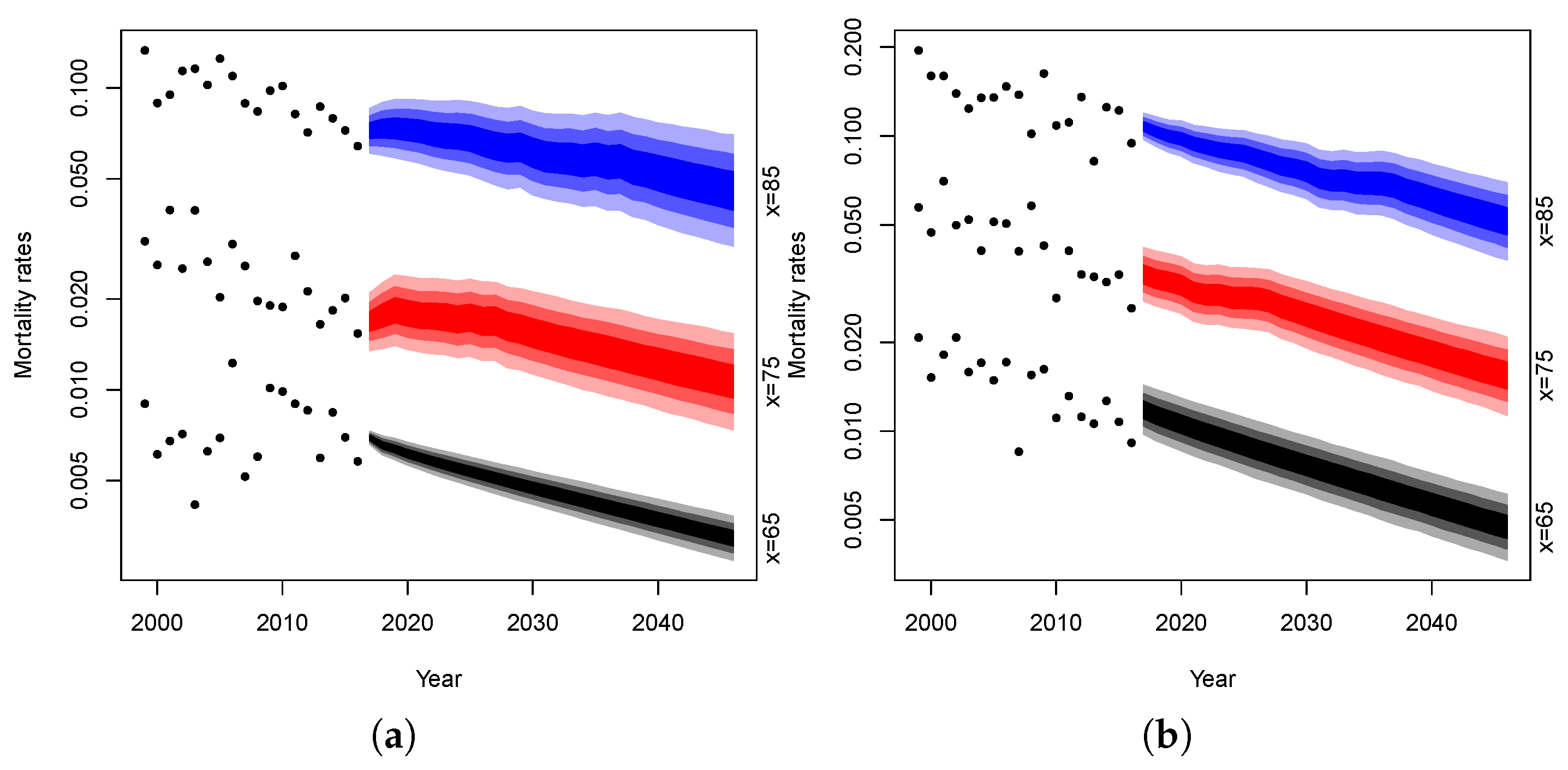
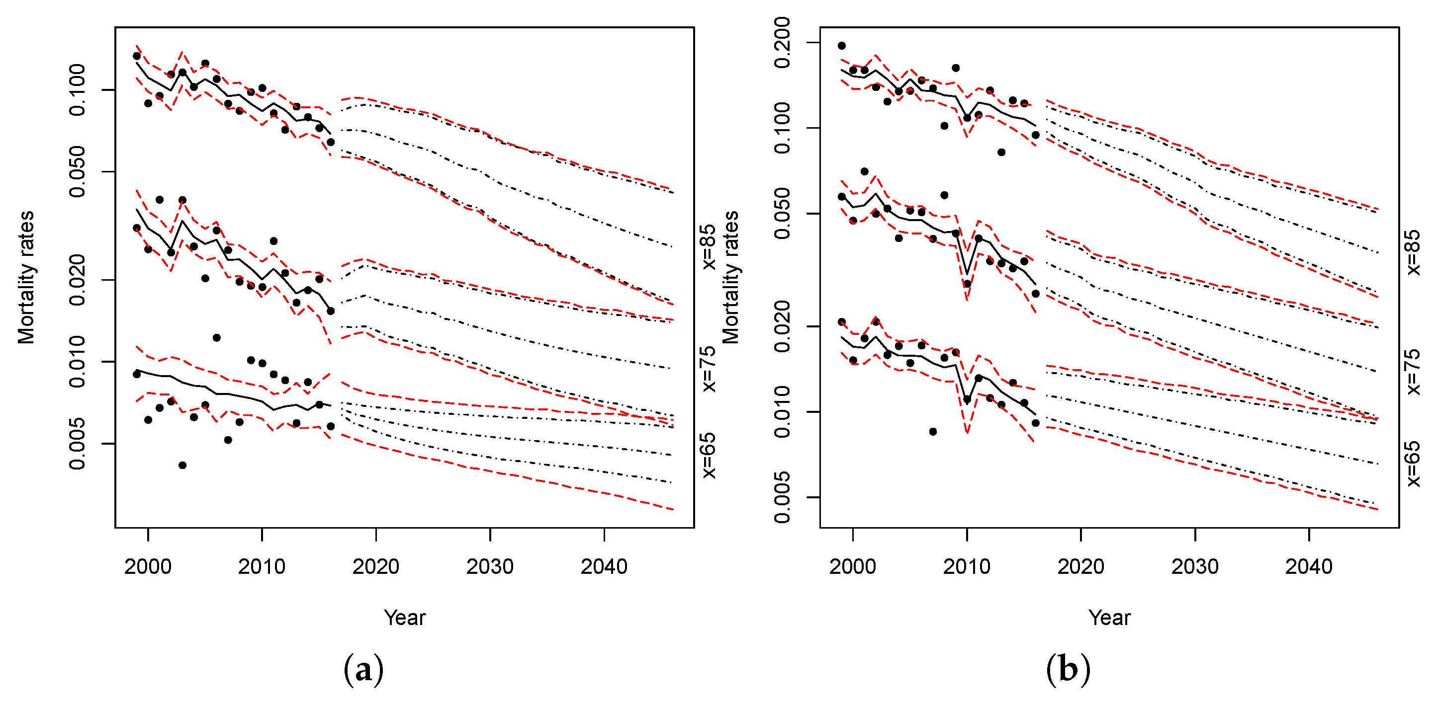
The following simulations are obtained by projecting each dynamics parameters up to 2046 and combining them in accordance with the model structure. It should be noted that we project mortality on a temporal horizon of 30 years even if the models are fitted on only 18 years of data. Obviously, this can be dangerous and the projections could be affected by significant uncertainty. On the other hand, we believe that making projections for a time horizon of less than 30 years would not allow us to appreciate the differences in the projections of the different models considered. We, thus, produce 10,000 simulations of mortality rates and plot their confidence intervals for both genders at age 65, 75 and 85. Fan charts of the simulated rates are reported in Figure 13 and Figure 14.

In the figures, the dotted lines represent mortality rates observed in Malta at age 65, 75 and 85 years, respectively. The blue area represents the confidence intervals of the projected mortality rates at age 85 over the forecast horizon and the gradation of color denotes different percentiles: the darkest area between 25% and 75%, the medium between 10% and 90%, the lightest between 2.5% and 97.5%. The red area refers to the confidence intervals at age 75 and the black one at age 65.

It can be noted that the projections obtained are characterized by a reasonable uncertainty level for both the male and female population. Moreover, the mortality evolution seems to be biologically reasonable. Following Cairns et al. (2006), we consider biologically unreasonable: “a forecasting model that gives rise to the possibility of period mortality tables that have mortality rates falling with age” or “long-run mean reversion around a deterministic trend”.

4.3. Parameters Uncertainty

The uncertainty in mortality forecasts has different origins. For example, previous prediction intervals do not take into account the uncertainty arising from estimated model parameters. Parameter uncertainty assumes an important role when dealing with incomplete data, short historical series or data referring to small populations as in our application. For this reason, we include this source of uncertainty in the analysis. Bootstrap procedures are often used for this purpose: B samples are produced according to the distribution of the data and B sets of parameters are estimated on them; they are then used to produce confidence and prediction intervals.

Between the different bootstrap techniques, we choose the semi-parametric bootstrap introduced by Brouhns et al. (2005). It is based on the generation of B samples of deaths from a Poisson distribution with mean ${\widehat{d}}_{xt}$ (the fitted number of deaths by age and year). We generate 10,000 bootstrapped samples from the fitted values of the models.

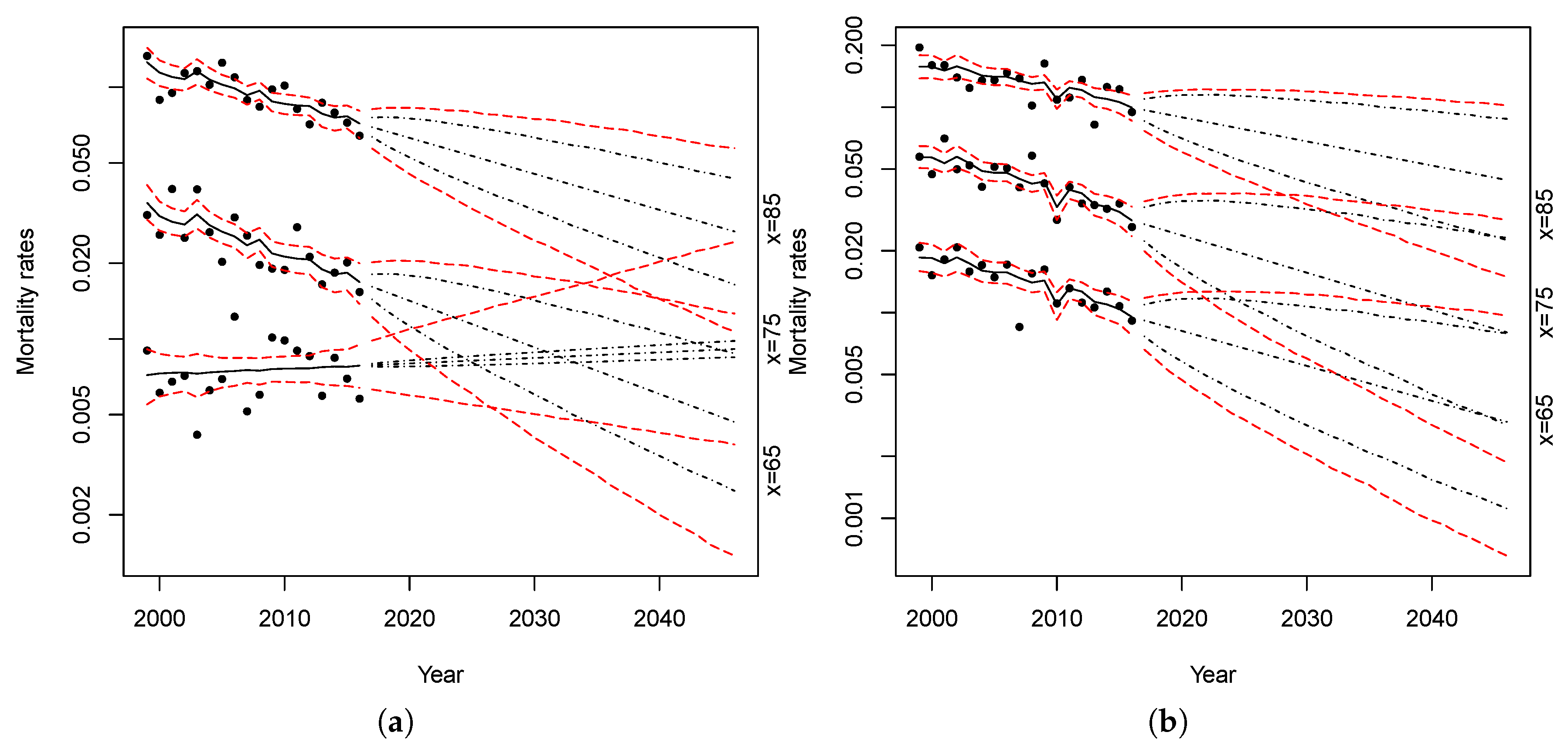
Figure 15 and Figure 16 show the simulations of the proposed models. The red lines represent the confidence intervals of the projected mortality rates with parameter uncertainty at 2.5% and 97.5%, while the black lines represent the confidence intervals without parameters uncertainty.

Comparing the forecast intervals, both models show a small level of parameter uncertainty. The parameter uncertainty is slightly higher only when we apply the models to females at lower ages.

In order to test to what extent the proposed procedure has succeeded in reducing the uncertainty related to the prediction of small populations mortality, we have applied a classic Lee–Carter (with one time factor) and an Age-Period-Cohort model on the Maltese data4. We then produced 10,000 simulations with parameter uncertainty. Results are shown in Figure 17 and Figure 18.

Comparing the bootstrapped projections obtained from the RH–LC and Plat–LC model (Figure 15 and Figure 16, respectively) with those obtained from the application of the standard Lee–Carter model (Figure 17) or those resulting from the application of the APC model (Figure 18), we can see that the uncertainty of predictions, or rather the width of the prediction intervals, is wider in the latter two cases. This is due to the fact that the reliability of traditional models could be reduced when applied to small populations because of the variability in observed data, while the models proposed in this paper considerably reduce the uncertainty of predictions.

Furthermore, as can be noted in Figure 17 looking at the evolution of the female death rate at age 65, a simple traditional model applied on a small population can produce biologically implausible results—for instance, it may happen to obtain mortality rates that are greater at younger ages than at older ages.

To highlight the reduction of uncertainty implied by the application of the proposed models, the confidence intervals amplitude for Maltese death rates, with 10,000 simulations with parameter uncertainty, are calculated with respect to their central trajectories for the year 2046. For each of the four models considered, the results are shown in

Table 11. Relative amplitude of prediction intervals for female Maltese death rates in 2046 with different mortality models.

Age	LC	APC	RH–LC	Plat–LC
65	225.77%	166.87%	74.66%	51.87%
75	232.54%	167.18%	90.75%	82.10%
85	169.40%	163.49%	100.23%	90.55%

and

Table 12. Relative amplitude of prediction intervals for male Maltese death rates in 2046 with different mortality models.

Age	LC	APC	RH–LC	Plat–LC
65	291.50%	209.40%	76.47%	63.34%
75	319.79%	205.04%	80.76%	68.43%
85	192.27%	206.97%	71.84%	65.93%

for females and males, respectively.

As shown above, the Plat–LC model interval variations are smaller than those of the other models. The interval variations of the LC model at age 65 (for both females and males) and at age 75 for males are more than four times greater than those of the Plat–LC. They are about three times greater at age 75 for females and at age 85 for males. Finally, they are about two times greater at age 85 for females. The Plat–LC model also reduces the uncertainty of projections compared to the APC single model, albeit to a lesser extent.

The reduction of uncertainty obtained with the RH–LC model is smaller than that obtained with the Plat–LC, although remarkable.

5. Conclusions

Performing mortality projections for a small country is a challenging issue due to the characteristics of the population and the available data. The observed mortality rates of a small population are characterized by a great volatility, dataset often available for a relatively short period and some data could be missing. As a consequence, the use of standard mortality models is not appropriate.

In this paper, we have dealt with the problem of Maltese mortality projections with a specific attention to older adults, which is also the age-group of greatest interest in actuarial applications: e.g., in pricing, reserving and risk management of life annuity portfolios or pension funds. Recent proposals in the literature suggest that the small population mortality can be modeled starting from the mortality of a bigger one (the reference population) adding a spread. Therefore, we have adopted a two-parts mortality model: a trend component, derived from a reference population, and a spread component.

We have first identified the reference population both by comparing some mortality indices and by identifying the optimal population mix that better approximate the death rates of the small population. From the analysis, it emerges that the best solution is to adopt the UK population as the reference one.

In the second step, we estimate the model for the reference population and for the spread and fit the two-part model to Maltese data. Finally, we obtain the mortality projections, also taking into account the parameter uncertainty through a bootstrap technique.

Both the adopted models produce biologically reasonable projections. Moreover, comparing the results obtained with the two proposed models with those obtained by applying standard models, it appears clearly that the adopted procedure allows us to drastically reduce the uncertainty in mortality rates projections. The differences between the results of our models are not so large. Thus, at first, we can conclude that the model risk is not an important issue. However, alternative models should be considered in order to better asses model risk.

Future research developments could be:

• to consider other methodologies for bootstrap as, for instance, the sieve bootstrap proposed by D’Amato et al. (2012) to capture the dependency risk produced by the presence of spatial dependence across age and time;
• to extend our analysis by considering other models for the reference and/or the small population (e.g., a two-part model obtained mixing models of the Cairns–Blake–Dowd family);
• to use the simulated death rates obtained with the proposed models in order to measure the longevity risk in the Maltese pension system;
• to test the effectiveness of the proposed models on other small populations, e.g., other small countries of the European continent.

References

- Ahcan, Ales, Darko Medved, Annamaria Olivieri, and Ermanno Pitacco. 2014. Forecasting mortality for small populations by mixing mortality data. Insurance: Mathematics and Economics 54: 12–27. [Google Scholar] [CrossRef]
- Antonio, Katrien, Sander Devriendt, Wouter de Boer, Robert de Vries, Anja De Waegenaere, Hok-Kwan Kan, Egbert Kromme, Wilbert Ouburg, Tim Schulteis, Erica Slagter, and et al. 2017. Producing the Dutch and Belgian mortality projections: A stochastic multi-population standard. European Actuarial Journal 7: 297–336. [Google Scholar] [CrossRef]
- Benjamin, Bernard, John H. Pollard, and Herbert W. Haycocks. 1993. The Analysis of Mortality and Other Actuarial Statistics. London: The Institute of Actuaries and The Faculty of Actuaries. [Google Scholar]
- Bongaarts, John. 2005. Long-range trends in adult mortality: Models and projections methods. Demography 42: 23–49. [Google Scholar] [CrossRef] [PubMed]
- Booth, Heather, Rob J. Hyndman, Leonie Tickle, and Piet de Jong. 2006. Lee–Carter mortality forecasting: A multi-country comparison of variants and extensions. Demographic Research 15: 289–310. [Google Scholar] [CrossRef]
- Bravo, Jorge, and Joana Malta. 2010. Estimating Life Expectancy in Small Population Areas. Geneva: United Nations Economic Commission for Europe. [Google Scholar]
- Brouhns, Natacha, Michel Denuit, and Ingrid Van Keilegom. 2005. Bootstrapping the Poisson Log-bilinear Model for Mortality Projection. Scandinavian Actuarial Journal 3: 212–24. [Google Scholar] [CrossRef]
- Cairns, Andrew, David Blake, and Kevin Dowd. 2008. Modelling and management of mortality risk: A review. Scandinavian Actuarial Journal 2: 79–113. [Google Scholar] [CrossRef]
- Cairns, Andrew, David Blake, Kevin Dowd, Guy D. Coughlan, David Epstein, Alen Ong, and Igor Balevich. 2009. A quantitative comparison of stochastic mortality models using data from England and Wales and the United States. North American Actuarial Journal 13: 1–35. [Google Scholar] [CrossRef]
- Cairns, Andrew, David Blake, Kevin Dowd, Guy D. Coughlan, and Marwa Khalaf-Allah. 2011a. Bayesian Stochastic Mortality Modelling for Two Populations. Astin Bulletin 41: 29–59. [Google Scholar]
- Cairns, Andrew, David Blake, Kevin Dowd, Guy D. Coughlan, David Epstein, and Marwa Khalaf-Allah. 2011b. Mortality density forecasts: An analysis of six stochastic mortality models. Insurance: Mathematics and Economics 48: 355–67. [Google Scholar] [CrossRef]
- Chen, Liang, Andrew Cairns, and Torsten Kleinow. 2017. Small population bias and sampling effects in stochastic mortality modeling. European Actuarial Journal 7: 193–230. [Google Scholar] [CrossRef] [PubMed]
- Currie, Iain. 2006. Smoothing and forecasting mortality rates with P-splines. Talk given at the Institute of Actuaries, June 2006. Available online: http://www.macs.hw.ac.uk/~iain/research/talks/Mortality.pdf (accessed on 18 June 2018).
- D’Amato, Valeria, Steven Haberman, Gabriella Piscopo, and Maria Russolillo. 2012. Modelling dependent data for longevity projections. Insurance: Mathematics and Economics 51: 694–701. [Google Scholar] [CrossRef]
- D’Amato, Valeria, HSteven Haberman, Gabriella Piscopo, Maria Russolillo, and Lorenzo Trapani. 2014. Detecting common longevity trends by a multiple population approach. North American Actuarial Journal 18: 139–49. [Google Scholar] [CrossRef]
- Dowd, Kevin, Andrew Cairns, David Blake, Guy D. Coughlan, and Marwa Khalaf-Allah. 2011. A gravity model of mortality rates for two related populations. North American Actuarial Journal 15: 334–56. [Google Scholar] [CrossRef]
- Haberman, Steven, and Arthur Renshaw. 2011. A Comparative Study of Parametric Mortality Projection Models. Insurance: Mathematics and Economics 48: 35–55. [Google Scholar] [CrossRef]
- Human Mortality Database. University of California, Berkeley (USA), and Max Planck Institute for Demographic Research (Germany). Available online: www.mortality.orgorwww.humanmortality.de (accessed on 5 October 2018).
- Hunt, Andrew, and David Blake. 2017. Modelling Mortality for Pension Schemes. Astin Bulletin 47: 601–29. [Google Scholar] [CrossRef]
- Hunt, Andrew, and Andrés M. Villegas. 2015. Robustness and Convergence in the Lee-carter model with cohort effects. Insurance: Mathematics and Economics 64: 186–202. [Google Scholar] [CrossRef]
- ISTAT. 2001. Tavole di Mortalitá Della Popolazione Italiana per Provincia e Regione di Residenza. Available online: https://www.istat.it/it/files//2018/08/volume-tavole-mortalita-1998.pdf (accessed on 1 July 2018).
- ISTAT. 2015. Tavole di Mortalitá: Singole etá. Anno 2015. Available online: https://www.istat.it (accessed on 1 July 2018).
- ISTAT. 2016. Tavole di Mortalitá: Singole etá. Anno 2016. Available online: https://www.istat.it (accessed on 1 July 2018).
- Jarner, Søren Fiig, and Esben Masotti Kryger. 2011. Modelling Adult Mortality in Small Populations: The SAINT Model. Astin Bulletin 41: 377–418. [Google Scholar]
- Keyfitz, Nathan, and Hal Caswell. 2005. Applied Mathematical Demography. New York: Springer. [Google Scholar]
- Kleinow, Torsten. 2015. A common age effect model for the mortality of multiple populations. Insurance: Mathematics and Economics 63: 147–52. [Google Scholar] [CrossRef]
- Lee, Ronald D., and Lawrence R. Carter. 1992. Modeling and Forecasting U.S. Mortality. Journal of the American Statistical Association 87: 659–71. [Google Scholar] [CrossRef]
- Li, Johnny Siu-Hang, Rui Zhou, and Mary Hardy. 2015. A step-by-step guide to building two population stochastic mortality models. Insurance: Mathematics and Economics 63: 121–34. [Google Scholar] [CrossRef]
- Li, Nan, and Ronald Lee. 2005. Coherent Mortality Forecasts for a Group of Populations: An Extension of the Lee–Carter Method. Demography 42: 575–94. [Google Scholar] [CrossRef]
- Plat, Richard. 2009. On stochastic mortality modeling. Insurance: Mathematics and Economics 45: 393–404. [Google Scholar]
- Renshaw, Arthur E., and Steven Haberman. 2006. A cohort-based extension to the Lee–Carter model for mortality reduction factors. Insurance: Mathematics and Economics 38: 556–70. [Google Scholar] [CrossRef]
- Villegas, Andrés M., and Steven Haberman. 2014. On the Modeling an Forecasting of Socioeconomic Mortality Differentials: An Application to Deprivation and Mortality in England. North American Actuarial Journal 18: 168–93. [Google Scholar] [CrossRef]
- Villegas, Andrés M., Steven Haberman, Vladimir K. Kaishev, and Pietro Millossovich. 2017. A Comparative Study of Two-Population Models for the Assessment of Basis Risk in Longevity Hedges. Astin Bulletin 47: 631–79. [Google Scholar] [CrossRef]
- Villegas, Andrés M., Steven Haberman, Vladimir K. Kaishev, and Pietro Millossovich. 2018. StMoMo: An R Package for Stochastic Mortality Modeling. Journal of Statistical Software 84: 1–38. [Google Scholar] [CrossRef]
- Wan, Cheng, and Ljudmila Bertschi. 2015. Swiss coherent mortality model as a basis for developing longevity de-risking solutions for Swiss pension funds: A practical approach. Insurance: Mathematics and Economics 63: 66–75. [Google Scholar] [CrossRef]
- Wang, Hsin-Chung, Ching-Syang Jack Yue, and Chen-Tai Chong. 2018. Mortality Models and Longevity Risk for Small Populations. Insurance: Mathematics and Economics 78: 351–59. [Google Scholar] [CrossRef]
- Willets, Richard. 2004. The Cohort Effect: Insights and Explanations. British Actuarial Journal 10: 833–77. [Google Scholar] [CrossRef]