Experience Prospective Life-Tables for the Algerian Retirees


1
Centre for Research in Applied Economics for Development—CREAD, Algiers 16011, Algeria
2
Institut de Science Financière et d’Assurance—ISFA, Université Claude Bernard, 69007 Lyon, France
*
Author to whom correspondence should be addressed.
Risks 2019, 7(2), 38; https://doi.org/10.3390/risks7020038
Submission received: 31 December 2018
/
Revised: 22 March 2019
/
Accepted: 1 April 2019
/
Published: 4 April 2019
(This article belongs to the Special Issue New Perspectives in Actuarial Risk Management)
Abstract
:The aim of this paper is to construct prospective life tables adapted to the experience of Algerian retirees. Mortality data of the retired population are only available for the ages from 50 to 95 years and older and for the period from 2004 to 2013. The use of the conventional prospective mortality models is not supposed to provide robust forecasts given data limitation in terms of either exposure to death risk or data length. To improve forecasting robustness, we use the global population mortality as an external reference. The adjustment of the experience mortality on the reference allows projecting the age-specific death rates calculated based on the experience of the retired population. We propose a generalized version of the Brass-type relational model incorporating a quadratic effect to perform the adjustment. Results show no significant difference for men, either retired or not, but reveal a gap of over three years in the remaining life expectancy at age 50 in favor of retired women compared to those of the global population.
1. Introduction
Life expectancy is still improving in developing countries. However, this improvement may be different by subpopulations. Retirees are supposed to benefit from better healthcare and living conditions compared to the rest of the population. As a direct impact, their risk of mortality is assumed to be lower. Hence, the use of dynamic life-tables based on global population data may distort all calculations when used for managing pension plans. Under a Pay-As-You-Go (PAYG) retirement system, as in the case of Algeria, the expected benefits to be paid for retirees during their remaining life depends on their survival function, which could be significantly different from that of the global population. Accordingly, life tables reflecting the retirees’ mortality experience need to be produced and then projected in a way to expect the future longevity of retirees. In addition, in the absence of actuarial prospective life tables based on the insurance industry data, prospective life tables of retirees seem to be more appropriate for life-annuities pricing compared to the global population tables. Indeed, the survival function of annuitants is not assumed to be similar to that of retirees, but the gap should be smaller compared to that of the global population. Such an option can be adopted in the case of countries not having well adapted actuarial life tables. The actuarial life tables in Algeria, TV 97-99 and TD 97-99, are based on old global population data and with no consideration to future longevity. In all circumstances, using retirees’ experience-based life tables would provide a better risk estimation of the annuitants’ mortality compared to the tables currently in use.
However, even the literature on prospective mortality modeling is rich; the implementation of the proposed models is constrained by a set of data limitations. Usually, the length of the retirees’ mortality is not long enough to provide robust forecasts. The second limitation is due to the data size. Since they are based on reduced samples compared to the global population size, the calculated mortality rates can display important variations over time and age. In such a case, the use of the prospective mortality models such as the Lee–Carter (Lee and Carter 1992) or Cairns–Blake–Dowd models (Cairns et al. 2006) to predict the future mortality trends is not supposed to provide robust forecasts in all situations.
In the literature, several models have been proposed to deal with data limitation when forecasting mortality. Such an issue is not new, and some simplistic methods have been proposed starting in the 1970s. In 1978, the “Continuous Mortality Investigation CMI” was proposed to forecast the mortality specific to the insured population in the UK. The proposed method aims to estimate a periodic experience life table for which an improvement scale is applied to estimate the future evolution of the mortality specific to the insured population (CMI 1978). The so-called “improvement scale” consists of age-specific mortality improvement rates estimated from the recent observed years. A very similar method was adopted in the US during the 1990s (SOA 1995). Starting in 2003, stochastic mortality models have been used to project the annuitants experience mortality in the UK (CMI 2004). The improvement scale based methods are still used nowadays to model the longevity specific to the insurance industry in some countries, such as Canada (CIA 2014).
Following the contribution of Lee and Carter (1992), many generalized versions have been proposed not only to improve goodness-of-fit and predictive capacity of mortality models but also male–female coherence. In this sense, Li and Lee (2005) proposed the augmented common factor Lee–Carter (LC) model to produce male–female coherent mortality forecasts. Their idea consisted of using the LC model (Lee and Carter 1992) to forecast mortality for male and female populations. To make the two projections evolve in a coherent framework regarding the sex differential mortality, a common age–time factor is added to both models. Afterwards, the model was extended to include heterogeneous subpopulations other than the gender-based ones, leading to what we call two-population models or more broadly multi-population models. Multi-population models are oriented to model the mortality specific to each subpopulation with specific models incorporating some common components (e.g., the Joint-K model and the common factor LC model). Others have proposed to model and forecast the spread between subpopulations and global population or any other reference (Jarner and Kryger 2011; Hyndman et al. 2013; Villegas and Haberman 2014). Villegas and Haberman (2014) used an LC model to forecast the spread, while Jarner and Kryger (2011) decomposed it into two vectors similar to beta and kappa in the LC model. The product-ratio method proposed by Hyndman et al. (2013) is slightly different: by estimating a joint mortality surface for males and females and a corresponding sex ratio surface, both are estimated and forecasted using the LC model. In the same way, Li et al. (2015) proposed multi-populations models based on the Cairns–Blake–Dowd (CBD) model and variants (Cairns et al. 2006, 2009). Detailed descriptions of these models were reported by Villegas et al. (2017).
Forecasting the spread is only possible when the historical data length is long enough. Otherwise, the spread is modeled and supposed to keep invariant in the future. That said, the relationship between the book and the reference remains the same over time. In this sense, some methods were proposed to convene the case of limited datasets. Planchet (2006) proposed modeling the spread between the experience mortality and the reference using a linear regression similar to the Brass Logit system (Brass 1971). Starting from an experience mortality surface extended only over 11 years, he estimated a linear regression of the experience mortality rates, in Logit, in function of those issued from the French national life tables. The obtained regression allows deducing the future experience mortality rates from the national forecasts. The same method was reproduced by Kamega (2011) to forecast mortality specific to the insurance market in sub-Saharan African countries. Again, the French tables (TG05 and TGF06) were taken as a reference. Thomas and Planchet (2014) conducted a comparison of a set of methods that can be applied to model the spread between experience mortality and an external reference, including the Brass-type relational model proposed by Planchet (2006). Plat (2009) set the spread to be simply the experience mortality rates divided on the references rates. He decomposed the spread into two components related to age and time in a similar manner to Jarner and Kryger (2011). The age and time components were respectively fitted using linear regression and a zero-trend stationary time series model ARIMA(0,0,0). The reasoning behind the Plat model seems very similar to that proposed by Planchet (2006). Even calculated in different ways, the spread in both models is represented by a linear function across age, assumed to keep constant over time.
In this paper, far from conducting a comparative evaluation of all these methods, we intend to investigate the applicability of the Brass-type relational model proposed by Planchet (2006) with some adaptations to Algerian retirees’ data. The first adaptation consists in using the Algerian global population mortality surface as an external reference. The future improvement of the retirees’ mortality is assumed to follow a similar trend to that of the global population, even if different general levels can be displayed. Using the national life tables of the period going from 1977 to 2014, we perform coherent mortality forecasts for the male and female populations aged 50 years and older using the model of Hyndman et al. (2013). Both types of data are used in this paper as an external reference to adjust and to forecast the retirees experience mortality. The retirees’ data are available for ten years going from 2004 to 2013 and arranged in five-age intervals from [50,55[ to 95 years and older, for males and females. These data concern the observed number of deaths and the survivals number by the end of each year of the observation period. First, the five-age death rates are calculated and interpolated into age-specific deaths rates (ASDRs) and fitted independently for each year to reduce irregularities. Then, we estimate a logit-linear regression model between the experience rates and the reference ones for common age interval and time range. The quality of the adjustment of the experience mortality to the reference is evaluated by comparing the retirees observed deaths to the confidence bounds predicted by the adjustment model. To improve the quality of the adjustment if required, we propose using a logit-quadratic relational model to adjust the experience death rates to the reference. However, we avoid including higher-order polynomial models to reduce the plausibility of the experience rates compared to the reference in long run forecasts (Plat 2009).
2. Retirees Experience Mortality
2.1. Data
Before to go through a detailed description of our dataset, it would be appropriate to provide an overview of the retirement scheme from which this data is issued. The Algerian public retirement system is constituted by different regimes: a military regime, a regime dedicated to the high-level officials of the government, and a civil regime. This last one combines two schemes: a scheme for the salaried workers, managed by the “Caisse Nationale des Retraites (CNR)”1, and another one for the self-employed workers managed by the “Caisse Nationale de Sécurité Sociale des Non-Salariés (CASNOS)”2. The CNR covers over 90% of the retirees within the civil regime. It provides mainly two types of pension benefits: direct pension benefits (DPB) and survivors pension benefits (SPB).
As mentioned in the Introduction, retirees’ mortality data are available starting from the age of 50 years in our case. That is because the legal age of retirement is 60 and 55 years for men and women, respectively, but some options are offered to retire below those ages. First, a full retirement can be accessed after 32 years of contribution not depending on age. Early retirement is associated with 20 and 15 working years for men and women aged 50 and 45 years, respectively. In addition, women can get a one-year bonus for each birth to a limit of 3. Additionally, some categories can benefit a retirement age bonus: Moudjahidhine3, disabled workers, and workers in special nuisance conditions.
Our dataset is concerned with the direct pensions’ beneficiaries of the CNR during the period 2004–2013. The beneficiaries of survivor’s benefits were not included. The population at the end of each year and the observed deaths are arranged in five age intervals from [50,55[ to 95 years and older, by sex. We set () to be the number of deaths observed in the age interval during the year “” and () the population aged between and years old by the end of the year “”.
Mortality rates denote the observed numbers of deaths during the year divided by the population at risk during the same year. In the absence of detailed information about the different dates to events, date of entrance/exit in the sample and date of birth/death, the population at risk cannot be accurately estimated. The use of aggregated data leads to less accurate results under some simplifying assumptions.
Since we do not have any information about the flow of individuals into/from the considered portfolio, we estimate the exposure to the death risk by the population number by the mid-year , which may be approximated by the average between the surviving population at the beginning and the end of the year by using the following formula:
We consider the distribution of the population of retirees by the end of the year “”, = 2004, 2005, ... 2013. To estimate the population at risk by five age intervals in 2004, the population distribution at the end of the previous year, i.e., 2003, is needed. For simplification issues, it was deduced from that of the end of 2004 by applying the ratio of the population distribution by the end of 2005 on that of 2004. The observed number of deaths and the population at risk for each age interval [ and year are represented in Figure 1.
The number of deaths has grown following a linear trend until the age interval [75,80[ years for men and [80,85[ for women. Then, it decreases slightly beyond those ages. In concern of the distribution of retirees number by age, we observe that the age interval [60,65[ comprises the most important number of retirees, men and women.
Overall, we have an exposure to death risk of more than 11 million person-years along the period from 2004 to 2013, which represents an average of 1.4 million person-years per year and a total of 288,000 deaths were observed during the same period.
2.2. Estimation of the Experience Death Rates
The objective of this section is to estimate the mortality surface for males and females using the available data. Since detailed age data are not available, we estimate the mortality indicators following five age descriptions. The first indicator that we can estimate in such a case is the observed death rate in the age interval during the year () noted , which represents the number of deaths observed in the age interval and year () divided by the population at risk during the observation year . The calculation formula can be written as:
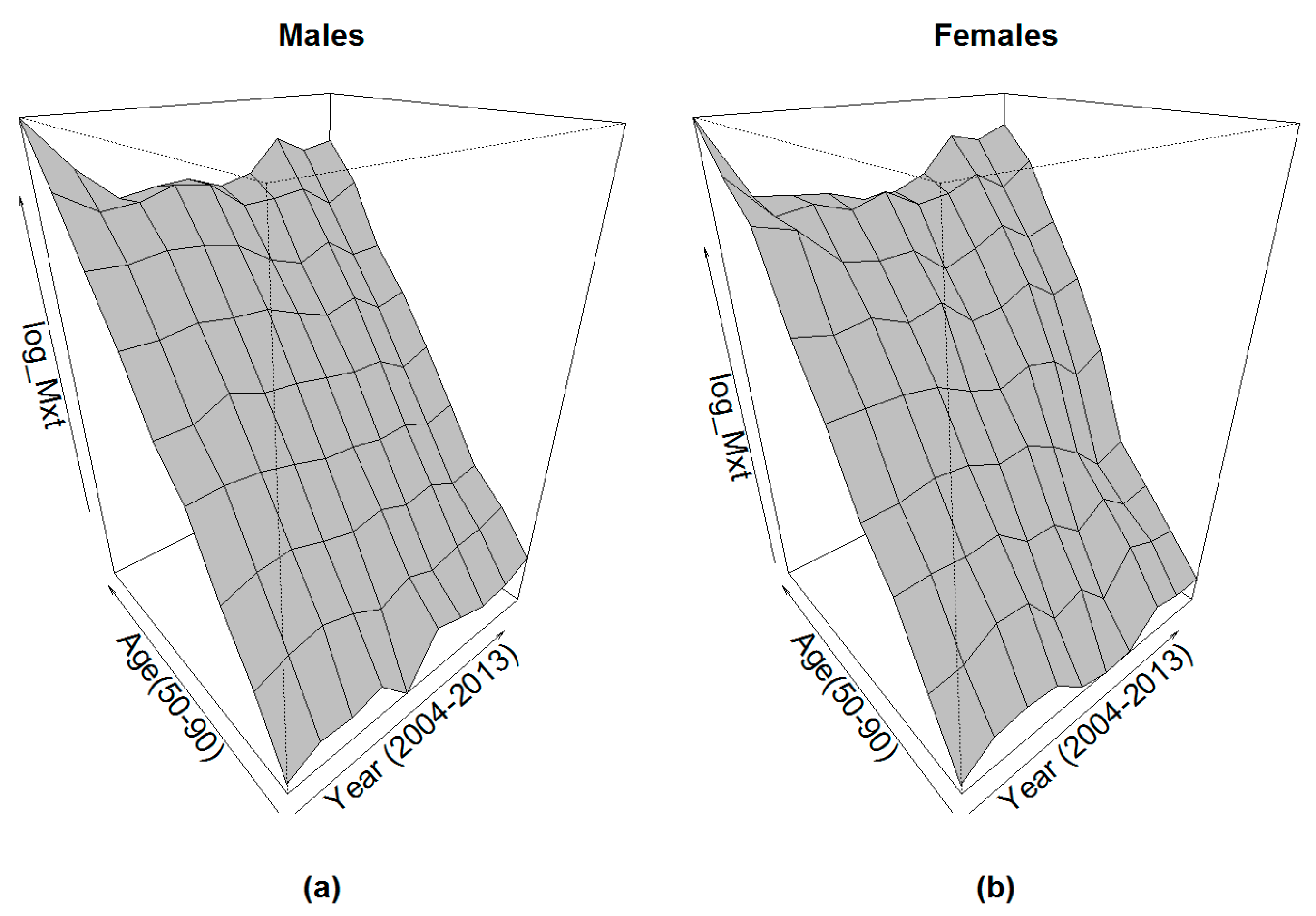
The obtained mortality surfaces are given in Figure 2.
We observe that the obtained mortality surfaces show relative stability until the ages of 80–85 years. Beyond this age, some irregularities can be observed due to the reduction of the deaths and the population exposed to risk.
2.3. Interpolating and Fitting the Experience Age-Specific Death Rates
The next step aims to construct detailed age life tables. The idea is to suppose that the central death rate of the age interval noted to be equal to the observed death rate corresponding to the same age and time points that we previously noted . We can write: . Then, we interpolate the ASDRs rates for = 50, 51, 52, …, 84. To this end, we use the quadratic model independently for each year “”:
The fitting process is oriented to minimize the weighted squared errors (WSE). The observed deaths can be used as a weight. The minimization problem can be written as follows:
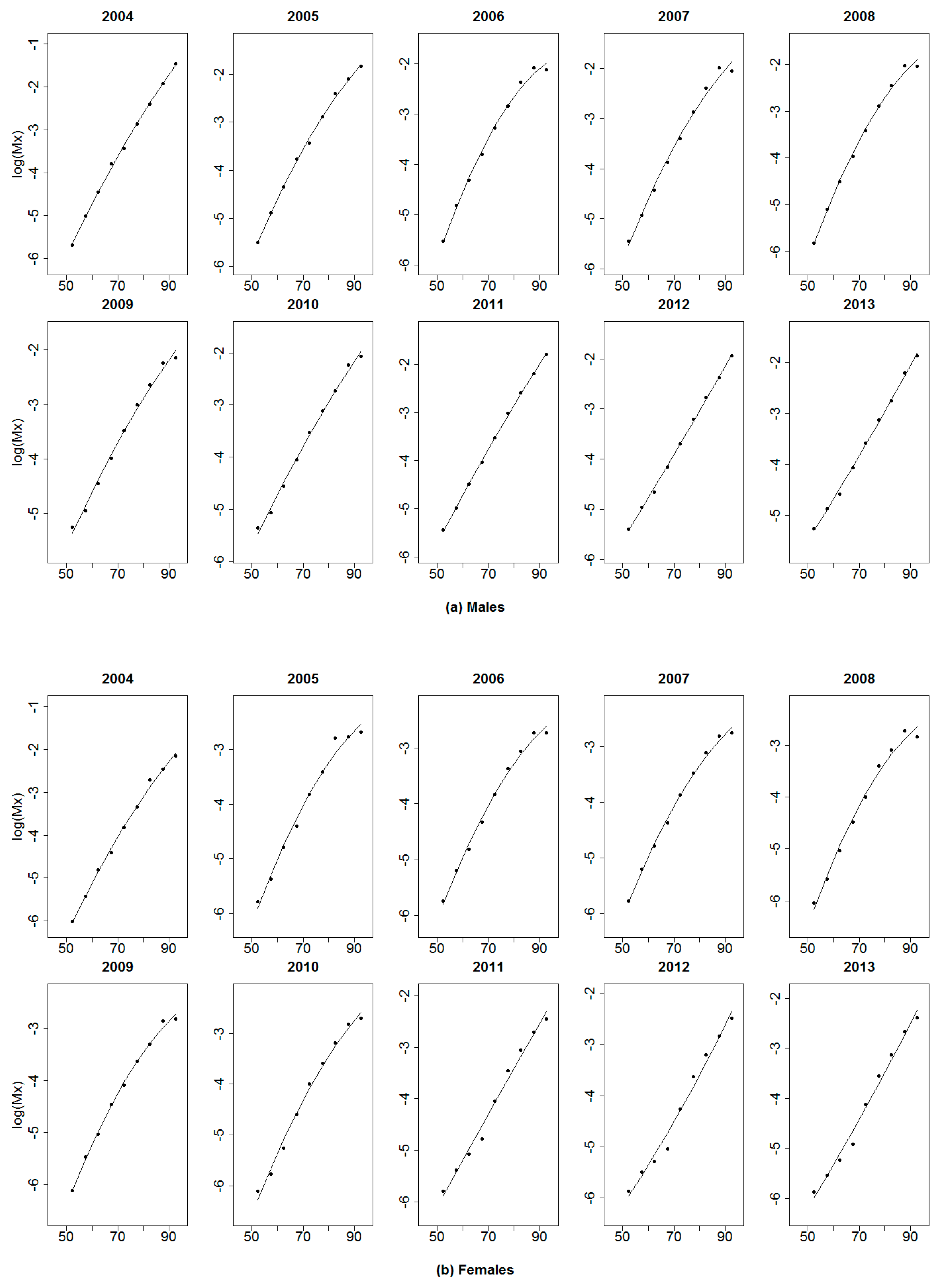
The fitting of the crude annual mortality curves is shown in Figure 3.
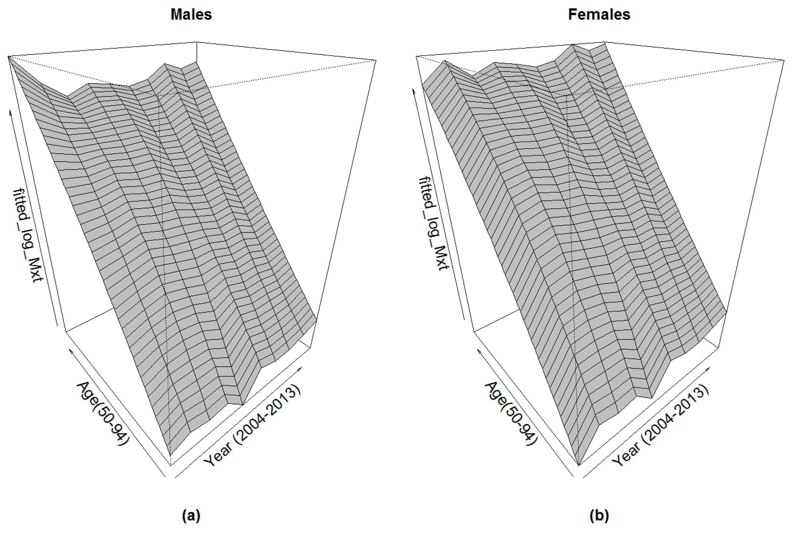
The quadratic fitting of the crude death rates aims to first interpolate the single age death rates and then reduce the irregularities caused by the reduced sample size for some age categories. As a result of this fitting, the annual life tables for the years were interpolated and smoothed. However, specific death rates at each age x as time series are still marked by some fluctuations, as shown in Figure 4.
3. External Reference Mortality
The length of the obtained mortality surface is limited and does not allow doing a robust forecast when the prospective mortality models are directly applied. For this, we need a consistent mortality reference to adjust the experience mortality. This adjustment consists of a regression allowing to pass in any condition from the reference mortality rates to the experience ones corresponding to the same age at the same year . Here, we propose to use the Algerian global population mortality as a reference.
3.1. Historical Mortality Surface of the Global Population
The Algerian life tables for the global population are published by the Office of National Statistics (ONS) starting from 1977. Mortality rates are given by five age intervals starting from 0 to around 75–80 for males, females and the combined population. These life tables were not published with an annual periodicity until 1998. That means there are some remaining years with no life table. Similarly, the closure age has been varying irregularly between the open age group of “70 years and older” to “85 years and older”. The implementation of mortality forecasting models requires the availability of a continuous historical mortality surface. Flici (2014) estimated the missing five-age mortality rates in the Algerian mortality surface.
To be able to project the experience mortality rates by an adjustment to an external reference, the reference mortality itself needs to include a projected part. Before proceeding to forecast the mortality of the global population aged 50 years and older, the age-specific mortality rates (ASMRs) are interpolated from the five age rates using the Karup–King method (see Shrock et al. 1993). The corresponding ASDRs are shown in Figure 5.
The aim of the adjustment of the experience mortality to a reference mortality surface is to ensure more robustness in forecasting. The main idea is to allow deducing the forecasted experience mortality rates from the projected reference rates. Thus, reference mortality rates must be projected. Flici (2016c) showed that the use of the prospective mortality models in an independent way does not guarantee coherent results regarding the male–female mortality ratio. For this, the use of coherent mortality models is highly recommended (Li and Lee 2005; Hyndman et al. 2013). Flici (2016b) conducted a comparison between these two models in the intention to project mortality for ages going from 0 to 79 years. It turned out from this comparison that the model proposed by Hyndman et al. (2013) leads to better results regarding the goodness-of-fit and the male–female coherence. Here, we present shortly the fitting and the forecasting process proposed by Hyndman et al. (2013), well-known as the product-ratio method, before using it to forecast mortality rates for the male and female populations aged 50 and older. Before, ASMRs have been converted to ASDRs using the approximation of Kimball (1960):
with representing the ASMR at age , and the corresponding ASDR.
The previous approximation assumes a uniform distribution of deaths along the age .
3.2. The Product Ratio Method
The coherent mortality forecasting method proposed by Hyndman et al. (2013) is based on the decomposition of the male–female mortality surfaces into two new components: a joint mortality function and a differential mortality function. The joint mortality function represents a common averaged surface for both males and females. It can be calculated by the geometric average of the male and female ASDRs at each year () and age () by the following formula:
with referring to both sex population, to males and to females.
The differential mortality function is represented by the rooted male–female mortality ratio. It can be calculated by:
The introduction of the root on the male–female mortality ratio is supposed to facilitate the reconstruction of the fitted male and female ASDRs by using the following formulas: and .
The joint mortality surface and the differential mortality function issued from the Algerian male and female mortality surfaces are shown in Figure 6.
3.3. Reference Mortality Coherent Forecasting
Next, we forecast the two components by using the model of Lee and Carter (1992), i.e., the joint-mortality surface and the differential mortality function.
3.3.1. Model Estimation
The log of the joint death rate at age and time is decomposed into three components:
The estimation process will be oriented to minimize the weighed sum of the squared errors (WSSE):
The weight is supposed to be the total deaths occurred at time and age for both males and females, while respecting the identifiability constraints: and .
For the sex ratio, we use:
The estimation process is oriented to minimize the weighed sum of the squared errors (WSSE):
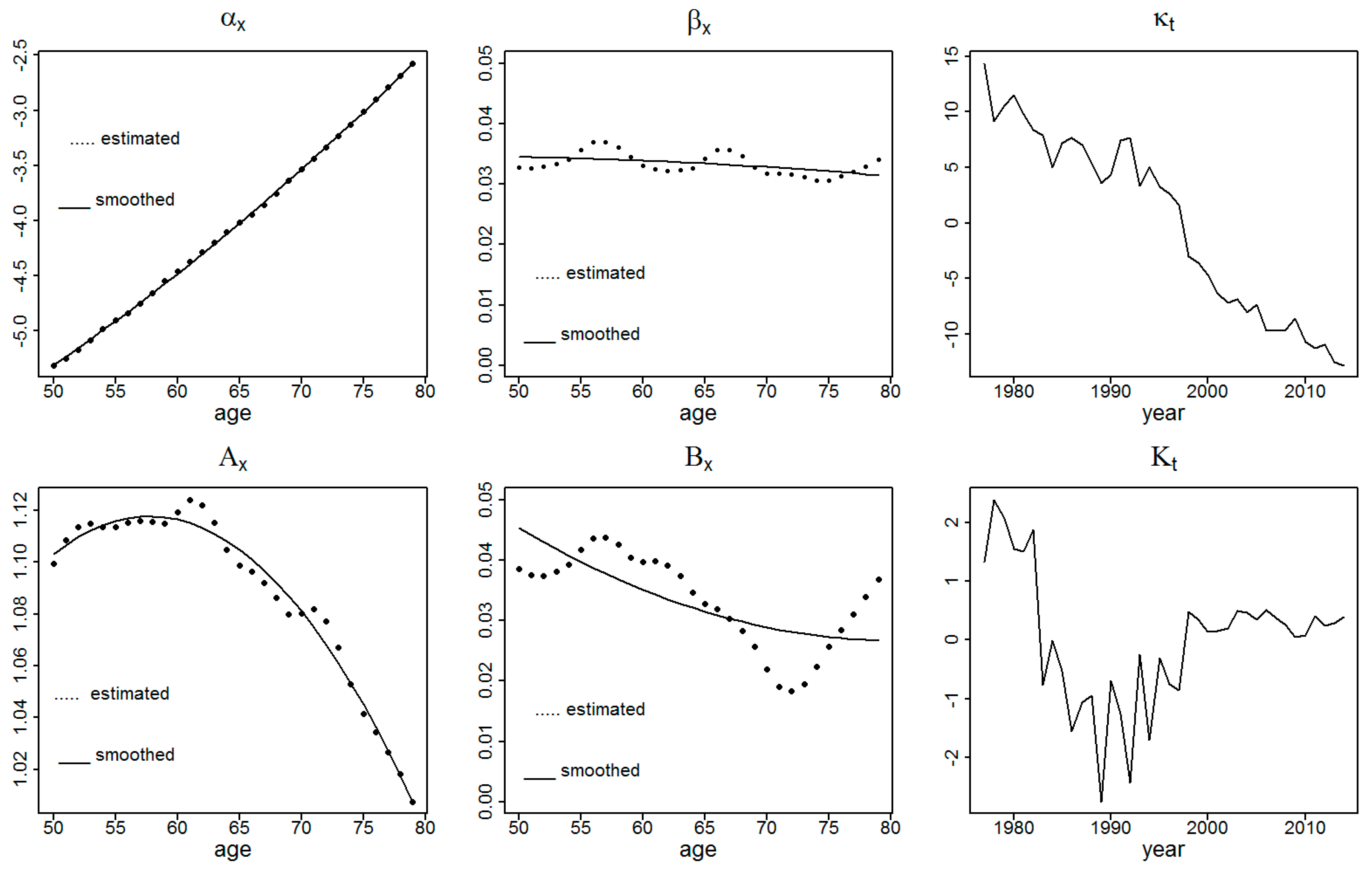
while respecting the identifiability constraints: and . The decomposition process led to the results presented in Figure 7.
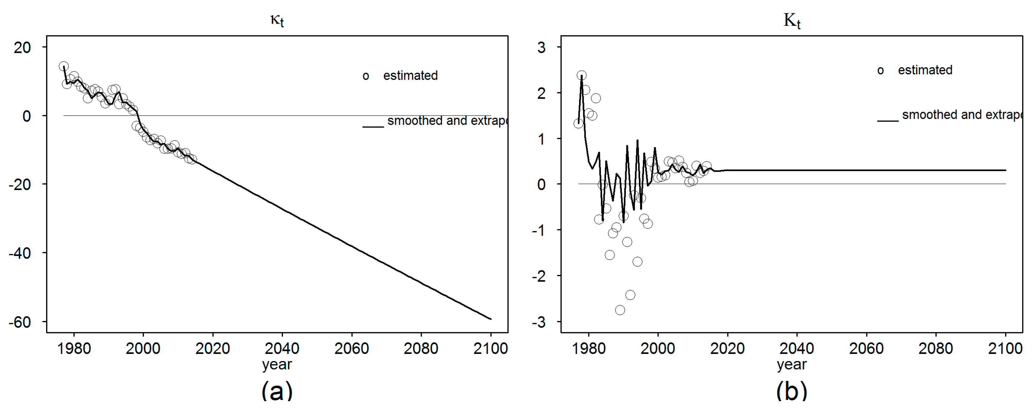
3.3.2. Time Indexes Forecasting
To forecast the mortality time index and the sex ratio variation index , many time series models can be used. A general review of modeling was presented by Flici (2016c). Here, we propose to compare three models: ARIMA(0,1,0), AR(1) and ARIMA(1,1,0). A random walk with drift is the most commonly used model to forecast mortality time index in the LC model (Lee and Carter 1992; Li and Lee 2005). The use of such a model requires that the historical evolution of the modeled parameter has a globally linear trend. This condition is verified in our case except some variations during the 1990s due to terrorism. The model can be written as: with as a drift and as an error term. The second model to be compared is the first-order Auto-Regressive model (AR(1)) with a constant, which can be written as: . Finally, it either models itself or models the differentiated series by using AR(1) with a drift. That leads to an ARIMA(1,1,0) for which we add a constant term and we can write: , which can be simply expressed by . The three models are compared based on the Mean Squared Errors (MSE) and the Bayesian Information Criterion (BIC).
These three models can also be applied to forecast the sex ratio time index (). The historical series shows a high irregularity during the period before 1998. The selection of the best forecasting model does not necessarily guarantee robust forecasts. The time interval to be used for model calibration has a relevant impact. When observing the initial series of , significant irregularities can be identified during the period 1992–1998. As a first intuition, we thought that excluding those years from the model calibration would lead to different results compared to when the whole period is considered. However, the three models display similar results whether the cited period was excluded or not. Hence, we prefer to keep including the whole period from 1977 to 2014 for model comparison. Contrary to the case of , the only way to obtain acceptable results with the sex ratio time index is the use of the recently observed trend only, i.e., from 1998 to 2014. The results are shown in Figure 8.
The extrapolated time indexes and combined with the age parameters allow reconstructing the projected mortality rates and sex ratios surfaces. According to this, the projected death rates can be obtained by with and the parameters of the LC model previously estimated and fitted and the projected mortality time index. Similarly, the projected age-specific sex ratio can be estimated using the formula: with and the age parameters already estimated and fitted and the projected time index.
Then, and using these two extrapolated parameters, males and females mortality surfaces can be deduced by and .
3.3.3. Old Age Mortality Extrapolation
The detailed ages mortality surfaces have until now been projected until 2100 for the age interval [50,79]. To extend the death rates to the older ages, we use the Coale–Kisker model (Coale and Kisker 1990). The Coale–Kisker method is based on a quadratic formulation of the growth of death rates beyond the age of 80, which implies a linear deceleration rate. Beyond the age of 80, passing from an age-specific death rate to the next one can be done by the formula:
is the annual average growth rate of death rates between 65 and 80, and is the slope of mortality growth rate deceleration which is supposed to decline following a linear trend. To estimate the slope “”, the authors imposed arbitrarily a closing constraint: and . This constraint does not imply that 110 years is defined as a surviving age limit as the case of the age 130 in Denuit and Goderniaux (2005). The constraint imposed by Coale and Kisker (1990) was meant to orient the old age mortality trend and avoid an eventual crossover between the male and female mortality curves.
For our application, we directly use a quadratic formulation of the Coale–Kisker method: . The model was calibrated to fit the death rates of the age interval [60,79] with imposing a constraint about the survival age limit, which is supposed to be 120 years old. This method was explained in detail by Flici (2016a).
3.4. Reference Mortality Extended and Forecasted Surface
After having projected the reference ASDRs for the age interval [50,79] until 2100, and having extrapolated them to the ages beyond 80 years, we can use the resulting surfaces, shown in Figure 9, as a reference to adjust and then forecast the experience mortality.
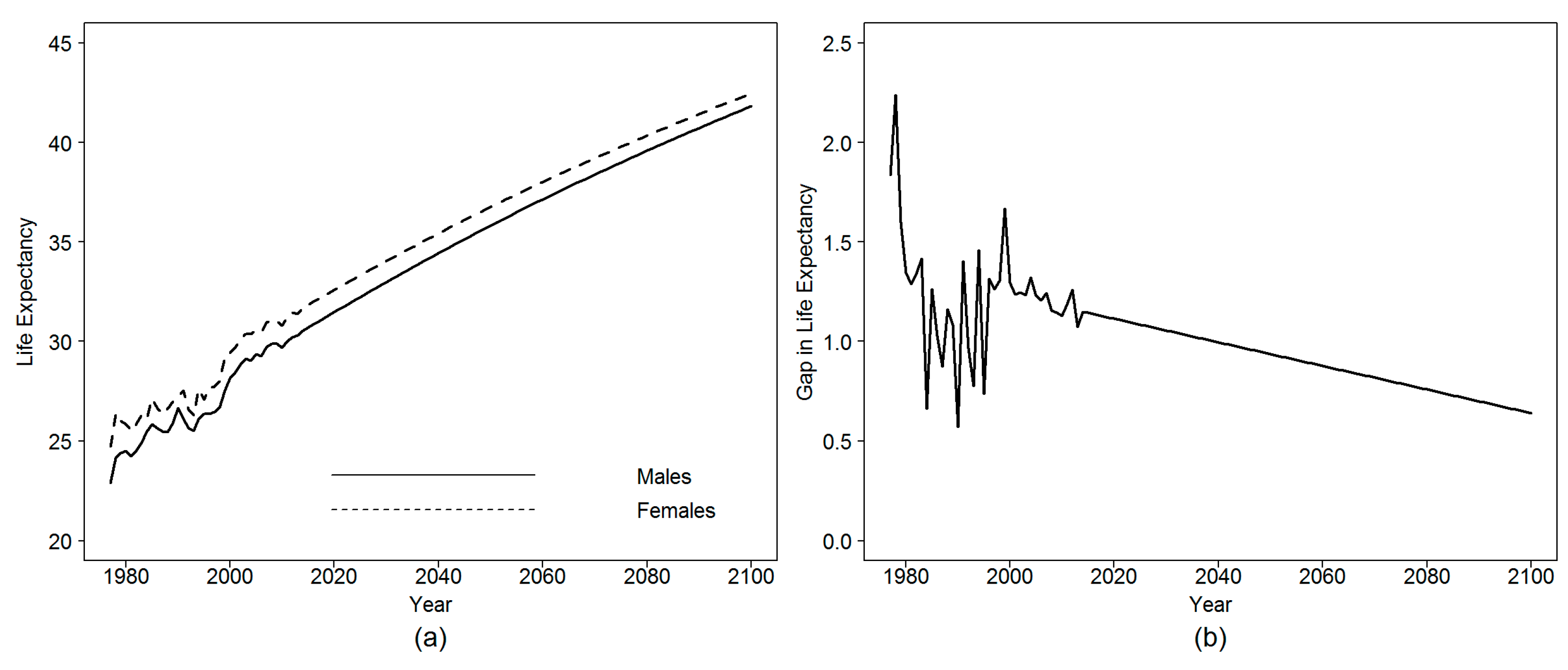
The projected mortality surfaces for males and females show a high regularity. The resulting projections about the remaining life expectancy at age 50 for males and females are shown in Figure 10. In addition, the figure illustrates the expected evolution of the sex gap in life expectancy at age 50.
The remaining life expectancy at age 50 for males is expected to increase from 30.5 in 2014 to 35.9 and 41.8 years in 2050 and 2100, respectively. For females, it is assumed to rise from 31.7 to 36.8 in 2050 and then to 42.5 years by 2100. The male–female gap in life expectancy will decrease from 1.14 to 0.65 year between 2014 and 2100.
4. Adjustment to an External Reference
The forecasting of the experience mortality rates by an adjustment to an external reference can be made through the estimation of the adjustment model and then using the resulted parameters to deduce the future experience rates from the forecasted reference rates. Let be the fitted ASDRs for age at time for the reference population and the fitted ASDRs related to the retired population. We remind that, until now, were projected until 2100. are only available for the period from 2004 to 2013. The adjustment model needs to be estimated on common age interval and time range connecting the experience and the reference surfaces. In our case, the experience mortality rates are available for the ages from 50 to 94 during the years from 2004 to 2013, while the reference rates are provided for ages from 0 to 79 along the period from 1977 to 2014. Consequently, the age interval [50,79] as well as the period from 2004 to 2013 can be considered as common age and time intervals, respectively. To improve the quality of the adjustment, a comparison is conducted between the original Logit-linear regression model proposed by Planchet (2006) and a generalized Logit-quadratic version.
4.1. Logit-Linear Regression Model
We remind that the Logit-linear regression model is based on the expression of the Logit of the experience death rates in function of the Logit of the reference death rates. That can be formulated as:
with γ and δ being the parameters of the linear regression model and an error term normally distributed. The model is estimated by minimizing the sum of squared errors (SSE) between the observed and the predicted experience death rates:
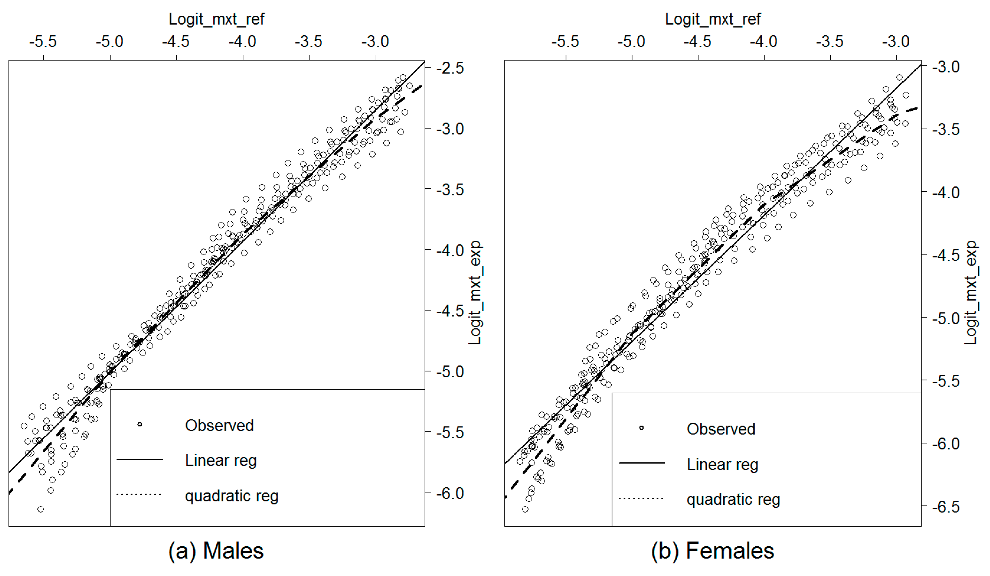
Figure 11 shows the obtained results.
We observe that the linear equation does not fit well the regression of the experience death rates on the reference ones. The regression seems to have a quadratic shape more relevant in the case of females. To evaluate the quality of the linear regression and its capacity to predict the experience death rates starting from the reference ones, we compare the observed deaths to those expected by the model. For this, the expected rates must be considered in respect to an error threshold beyond which the model is qualified inappropriate. That returns to the estimation of the confidence interval of the predicted death rates and the numbers of deaths.
We remind that the initial data were provided by five age intervals. For comparability issues, the deaths expected by the regression following a detailed age description, need to be arranged into five age intervals.
If we denote the annual average number of deaths observed in the age interval during the period from 2004 to 2013 and the corresponding population at risk, the crude death rates averaged on the period from 2004 to 2013 can be calculated as . On the other side of the comparison, the predicted number of deaths that we denote can be calculated by multiplying the adjusted death rates by the observed population at risk . We can write: . The can be averaged on the for “” going from 2004 to 2013. For each year “”, can be reconstructed using a geometric mean of the ASDRs at the detailed ages . With equal to 5, we can write:
with denoting the ASDR at age (going from to ) and year .
If we consider six age intervals for which the observed and the expected deaths are to be compared, the confidence bound must be calculated simultaneously for the six points. That recalls the notion of confidence bound, which is different from a confidence interval that can be estimated independently for each of the six age intervals. Here, we follow the methodology proposed by Planchet and Kamega (2013) on the estimating of confidence bounds for single age death rates. We adjust the proposed formula to suit the case of five-age death rates.
Estimating a confidence interval at a confidence level of 1 − for , which is supposed to be normally distributed, aims that there is a probability 1 − that the real death rate is comprised in the confidence interval:
with ) representing the () quantile of the reduced centered normal distribution.
Contrary to confidence intervals designed for the case of independent estimates, the confidence bounds consider the probability that all observed values are simultaneously within the corresponding confidence intervals. Accordingly, if there were a probability that is within its confidence interval, there would be a probability that a “” number of independent observations are simultaneously within their respective confidence intervals with . The confidence bound can be then calculated by:
Here, the confidence bounds have been estimated for an overall confidence level of corresponding to local confidence levels at each age group of
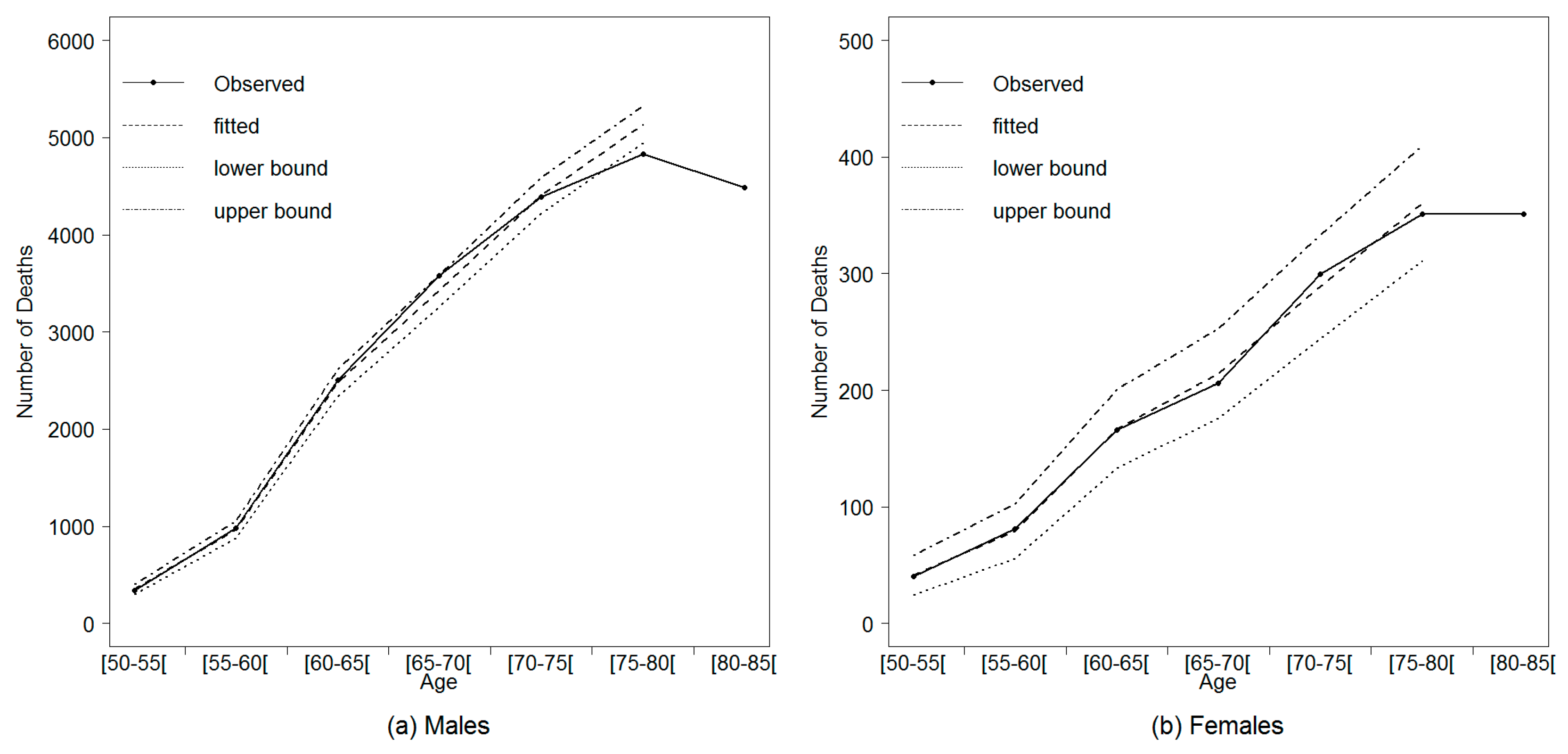
The confidence bounds calculated on the number of deaths (averaged on the period from 2004 to 2013) predicted by the linear regression are represented in Figure 12 as well a comparison to the observed deaths.
For females, we observe that the observed numbers of deaths are located within the confidence bound at all the age intervals. For males, the confidence bound fails to predict the observed numbers of deaths at the age intervals [65,70[ and [75,80[. That said, the variability of the experience mortality rates has not been correctly captured by the linear regression model.
4.2. The Logit-Quadratic Regression Model
To improve the quality of the adjustment, we propose a slight adaptation of the regression model to capture the curvature of the cloud points. The regression of the experience death rates on the reference rates is supposed to be expressed by a two-order polynomial function:
where , and are the regression parameters and is an error term.
Figure 13 shows the quadratic regression results compared to those previously obtained using the linear regression model.
To evaluate the quality of quadratic adjustment, we compare the distribution of the observed deaths to those predicted by the model. The recalculated confidence bounds are presented in Figure 14.
We observe that the Logit-quadratic model fits the pattern of the experience mortality rates in function of the reference ones better than the linear regression. The observed numbers of deaths are within the confidence bound at all ages for both males and females.
4.3. Retired Population Dynamic Life Tables
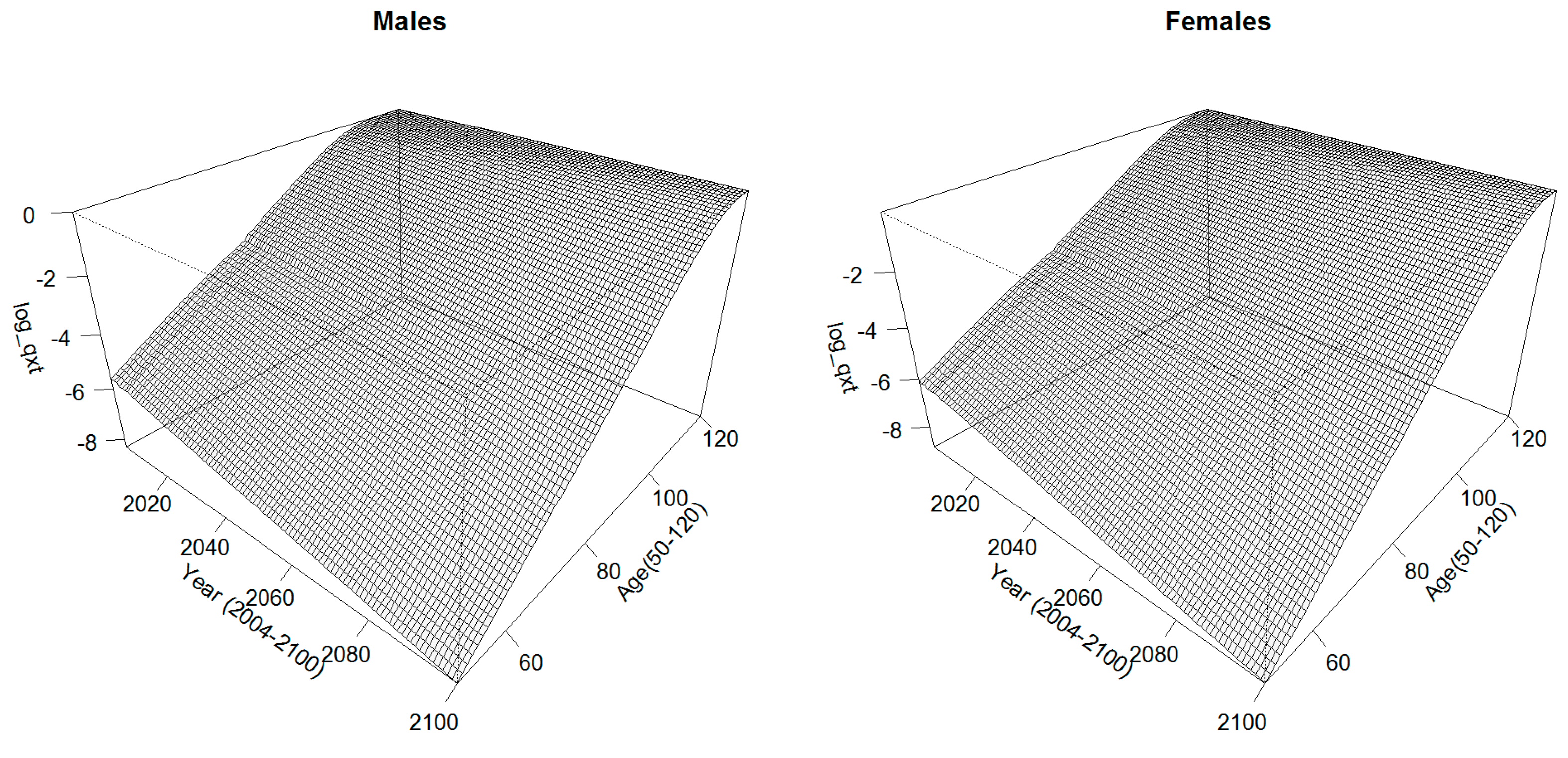
Using the coefficients of the quadratic regression model, the Logit of the retirees’ experience ASDRs can be deduced from those of the reference population already projected until 2100 for the age interval [50,79]. The ASDRs for the ages beyond are extrapolated using the Coale–Kisker model (Coale and Kisker 1990). Figure 15 shows the extrapolated mortality surfaces.
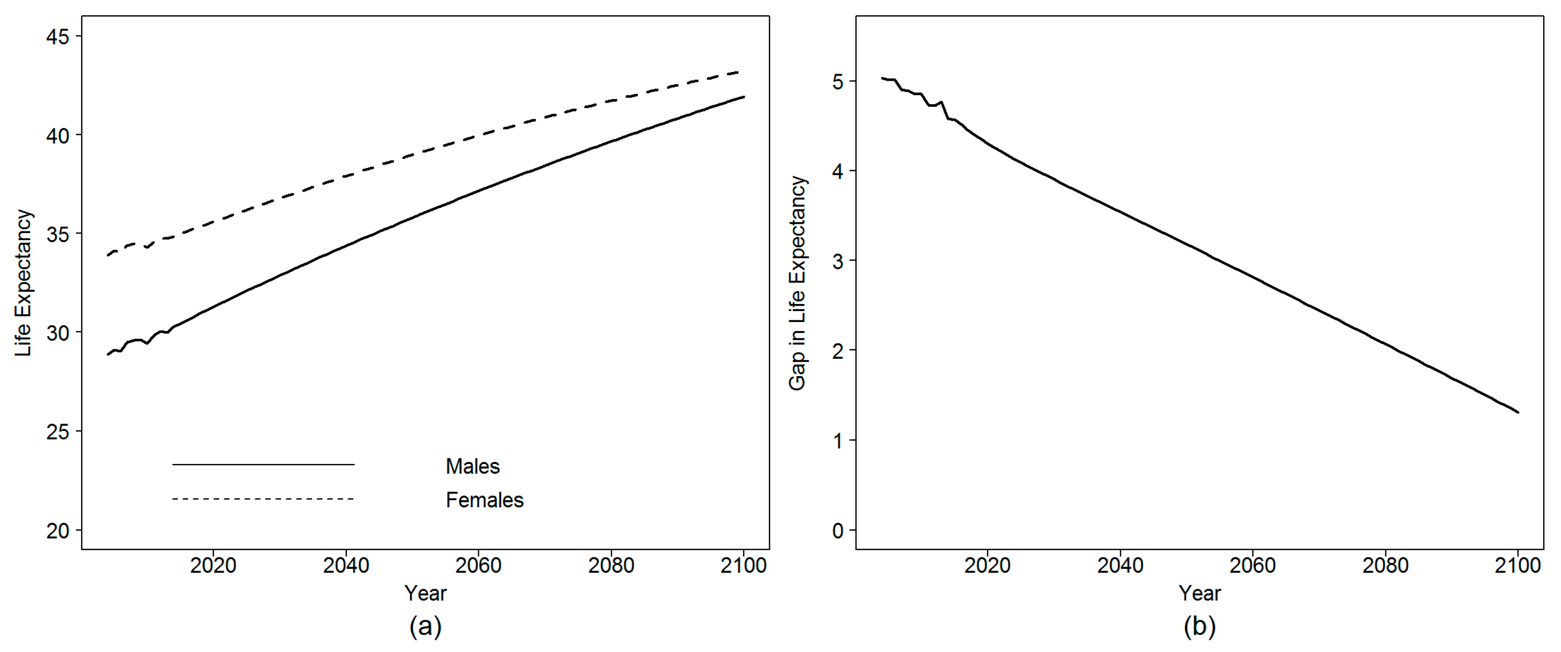
According to the forecasting results, the female life expectancy at age 50 is supposed to increase from 34.8 in 2014 to 39 and 40.9 in 2050 and 2070, respectively. For males, this value is expected to rise from 30.4 in 2014 to 35.8 and to 38.5 in 2050 and 2070, respectively. The sex gap in life expectancy at age 50, which was 4.4 in 2014, is expected to decrease to 2.4 by 2070. Figure 16 shows the obtained results in more details.
When we compare the obtained results to the global population life expectancy, significant differences arise when comparing males and females. Figure 17 gives a comparison in this sense.
According to Figure 17, there is no significant difference between the global and the retired population in terms of remaining life expectancy at age 50 in the case of males. The average gap is nearly five months during the whole observation period in favor of the global population. For females, the life expectancy of the retired women is 3.16 years higher than that of the female global population in 2014. This gap is expected to decrease to a value of 2.2 and 1.7 in 2050 and 2070, respectively.
There are two possible explanations for this last finding. The first explanation assumes that working has a positive effect on the female population contrary to men. For men, living conditions are not different whether they are insured or not. Adversely, working women have better and healthier living conditions compared to the rest of the female population. Such an assumption is supported by the fact that working women are more concentrated in un-risky activity sectors (services and administration) compared to men (ONS 2014). The second alternative supports the assumption that the ONS underestimates the life expectancy of the global female population. This last finding is sustained by the results of Flici and Hammouda (2016). When analyzing the data issued from the Multi Indicators Cluster Survey4 MICS2012, which focused on the period from 2008 to 2012, they found a gap of 3.9 years in life expectancy at birth between males and females of the global population. This result is near to the gap and the life expectancy obtained on the retired population. That let us suppose that the retired population (men and women) does not present any particularity in terms of remaining life expectancy compared to the global population and that ONS estimates about the female life expectancy could be inaccurate. To assess such assumption, we need to explore additional data sources (insurance companies, social security, etc.) and to investigate the methodology adopted by the ONS to estimate female mortality.
5. Conclusions
Two important points need to be considered when using life tables for managing retirement plans and pricing life annuities: one consists of the adjustment of the risk function to the experience of the targeted population, and the other aims to take the future improvement of this experience mortality into account. Being usually available for short periods, the data of the insured population make it hard to implement efficiently the prospective mortality models to predict future longevity. On the other side, using prospective life tables of the national population for actuarial calculations assumes that insured or retired people have the same age–mortality pattern as the global population. Such an assumption is not always realistic and may lead to risk misestimating.
In the late 1970s, the Continuous Mortality Investigation (CMI 1978) proposed to use actuarial life tables incorporating an improvement scale to predict the future mortality of annuitants in the UK. Later, this model was adopted in the US (SOA 1995) and Canada (CIA 2014). Due to the remarkable advancement in mortality stochastic modeling following the contribution made by Lee and Carter (1992), several models have been proposed to forecast mortality for different populations in a coherent way. Beginning with male–female coherent mortality forecasting (Li and Lee 2005) to two-population and multi-population models (e.g., Jarner and Kryger 2011; Hyndman et al. 2013; Villegas and Haberman 2014; Li et al. 2015), models were extended to forecasting limited mortality data by using relatively more important population data as a reference (e.g., Planchet 2006; Plat 2009; Planchet and Kamega 2013; Thomas and Planchet 2014). The idea behind these last models is to model the spread between the small population mortality, time-limited, and the reference, and then to derive the future evolution of the first from that of the second. This adjustment technique is highly suited for the case of the insured populations for which the observation history is limited in time.
In this paper, we have considered the case of the Algerian retirees within the salaried workers’ scheme. The experience data are available for the period 2004–2013, for males and females, and arranged in five age intervals from age 50 to 90 years and older. Our objective was to forecast the retirees experience mortality through an adjustment to an external reference using the Brass-type relational model proposed by Planchet (2006). To this end, we used the mortality surface of the Algerian male and female populations, available starting from 1977, as a reference. The model was estimated in the age interval [50,79] and for the period from 2004 to 2013, which correspond to the common age and time intervals between the global population and retirees’ data. Then, the estimated parameters were used to deduce the future experience death rates from the projected reference rates. Recall that the reference mortality, for males and females, has been projected in the future using the product-ratio model proposed by Hyndman et al. (2013).
To evaluate the performance of the Logit-linear model, we compared the observed deaths to the confidence bounds of the deaths predicted by the model. The comparison showed that the adjustment model failed to predict the experience mortality rates at some ages. Hence, we proposed a Logit-quadratic model to better fit the curvature of the distribution of the experience rates compared to the reference ones. The comparison of the observed deaths and the model predictions displayed a better quality compared to those provided by the Logit-linear model.
After having assessed its quality, the Logit-quadratic model was used to deduce the age-specific death rates of the retired population from the projected global population rates. The final results showed that the remaining life expectancy at age 50 of the male retirees is quite similar to that of men of the global population. Both indicators display a value of around 30 years in 2014 expected to improve to nearly 35.8 years in 2050. Adversely, the results reveal an important gap between retired women and women of the global population. The former have a higher remaining life expectancy at age 50, with three additional years. This gap is expected to narrow over time to two years by 2050.
Using the national life table to expect the future benefits to be paid for retirees during their remaining lifetime would lead to underestimating the real benefits owed to retirees and consequently to serious unexpected financial unbalance between contributions and retirement benefits. Indeed, such a finding remains true if retirees have better life expectancy compared to the global population. Accordingly, the case of retired women in Algeria cannot be ignored. Following the rise of the women’s employment rate in Algeria during the last two decades, one should expect a growing part of women among retirees in the future. Hence, neglecting the residual remaining life expectancy of the retired women will have an increasing impact on the financial imbalance of the retirement system. Nowadays, the calls for reforming the Pay-As-You-Go retirement systems in North Africa are mainly oriented to reduce the generosity of pensions (Ben Brahem 2009) and to ensure a stronger contribution–benefit linkage (Chourouk 2003). In such a context, the prospective life tables of the retired population will be necessary to evaluate the sustainability of retirement systems and to plan reforms.
Author Contributions
F.F.: data collection, models implementation, writing the first draft. F.P.: supervision, reviewing models implementation, reviewing the first draft. The two authors have equally contributed to the methodology of the paper.
Funding
This research received no external funding.
Conflicts of Interest
The authors declare no conflict of interest.
References
- Ben Brahem, Mehdi. 2009. Pension system generosity and reform in Algeria, Morocco and Tunisia. International Social Security Review 2: 101–20. [Google Scholar] [CrossRef]
- Brass, William. 1971. On the scale of mortality. In Biological Aspects of Demography. Edited by William Brass. London: Taylor and Francis. [Google Scholar]
- Cairns, Anrew J. G., David Blake, and Kevin Dowd. 2006. A two-factor model for stochastic mortality with parameter uncertainty: Theory and calibration. Journal of Risk and Insurance 73: 687–718. [Google Scholar] [CrossRef]
- Cairns, Andrew J. G., David Blake, Kevin Dowd, Guy D. Coughlan, David Epstein, Alen Ong, and Igor Balevich. 2009. A Quantitative Comparison of Stochastic Mortality Models Using Data from England and Wales and the United States. North American Actuarial Journal 13: 1–35. [Google Scholar] [CrossRef]
- Chourouk, Houssi. 2003. Pensions in North Africa: The need for reform. Geneva Papers for Risk and Insurance 28: 712–26. [Google Scholar] [CrossRef]
- Canadian Institute of Actuaries—CIA. 2014. Canadian Pensioners’ Mortality. Canadian Institute of Actuaries, Pension Experience Subcommittee–Research Committee. Final Report, Document 214013. Ottawa: Canadian Institute of Actuaries, February. [Google Scholar]
- Continuous Mortality Investigation—CMI. 1978. Proposed Standard Tables for Life Office. Report No. 3. London: Institute of Actuaries and Faculty of Actuaries. [Google Scholar]
- Continuous Mortality Investigation—CMI. 2004. Projecting Future Mortality: A Discussion Paper. Continuous Mortality Investigation, Mortality Sub-Committee, Working Papers, No 3. London: Institute and Faculty of Actuaries. [Google Scholar]
- Coale, Ansley J., and Ellen E. Kisker. 1990. Defects in data on old-age mortality in the United States: New procedures for calculating mortality schedules and life tables at the highest ages. Asian and Pacific Population Forum 4: 1–31. [Google Scholar]
- Denuit, Michel, and Anne-Cécile Goderniaux. 2005. Closing and projecting life tables using log-linear models. Bulletin de l’Association Suisse des Actuaires 1: 29–49. [Google Scholar]
- Flici, Farid. 2014. Estimation of the Missing Data in the Algerian Mortality Surface by Using an age-TIME Segmented Lee Carter Model. Paper presented at the Stochastic Modeling and Data Analysis Conference SMTDA, Lisbon, Portugal, June 12–15. [Google Scholar]
- Flici, Farid, and Nacer-Eddine Hammouda. 2016. Analyse de la mortalité en Algérie à travers les résultats de l’enquête MICS. Rapport technique. Alger: Centre de Recherche en Economie Appliquée pour le Développement CREAD. [Google Scholar]
- Flici, Farid. 2016a. Closing out the Algerian Life Tables: For More Accuracy and Adequacy at Old Ages. Paper presented at the IAA-ASTIN Section Colloquium, Lisbon, Portugal, May 31–June 2. [Google Scholar]
- Flici, Farid. 2016b. Coherent Mortality Forecasting for the Algerian Population. Paper presented at the Samos Conference in Actuarial Sciences and Finance, Samos, Greece, May 18–22. [Google Scholar]
- Flici, Farid. 2016c. Longevity and Life Annuities Reserving in Algeria: Comparison of mortality models. Paper presented at the IAA-Life Section Colloquium, Hong Kong, China, April 25–27. [Google Scholar]
- Hyndman, Rob J., Heather Booth, and Farah Yasmeen. 2013. Coherent mortality forecasting: The product-ratio method with functional time series models. Demography 50: 261–83. [Google Scholar] [CrossRef] [PubMed]
- Jarner, Søren Fiig, and Esben Masotti Kryger. 2011. Modelling adult mortality in small populations: The SAINT Model. ASTIN Bulletin 41: 377–418. [Google Scholar]
- Kamega, Aymric. 2011. Outils Théoriques et Opérationnels Adaptes au Contexte de L’assurance vie en Afrique Subsaharienne Francophone—Analyse et Mesure des Risques lies a la Mortalité. Ph.D. thesis, Risk Management, Université Claude Bernard, Lyon, France. [Google Scholar]
- Kimball, A. W. 1960. Estimation of mortality intensities in animal experiments. Biometrics 16: 505–21. [Google Scholar] [CrossRef]
- Lee, Roland D., and Lawrence Carter. 1992. Modeling and Forecasting U. S. Mortality. Journal of the American Statistical Association 87: 659–71. [Google Scholar]
- Li, Nan, and Roland D. Lee. 2005. Coherent mortality forecasts for a group of populations: An extension of the Lee Carter method. Demography 42: 575–94. [Google Scholar] [CrossRef] [PubMed]
- Li, Johnny Siu-Hang, Rui Zhou, and Mary Hardy. 2015. A step-by-step guide to building two population stochastic mortality models. Insurance: Mathematics and Economics 63: 121–34. [Google Scholar] [CrossRef]
- Office National des statistiques—ONS. 2014. Activité, emploi et chômage au 4° trimestre 2013. Available online: http://www.ons.dz/img/pdf/donnees_stat_emploi_2013.pdf (accessed on 28 August 2016).
- Planchet, Frédéric. 2006. Construction des tables de mortalité d’expérience pour les portefeuilles de rentiers—Présentation de la méthode de construction. In Note méthodologique de l’Institut des Actuaires. Paris: L’Institut des Actuaire. [Google Scholar]
- Planchet, Frédéric, and Aymric Kamega. 2013. Construction de tables de mortalité prospectives sur un groupe restreint: Mesure du risque d’estimation. Bulletin Français d’Actuariat 13: 5–34. [Google Scholar]
- Plat, Richard. 2009. Stochastic portfolio specific mortality and the quantification of mortality basis risk. Insurance: Mathematics and Economics 45: 123–32. [Google Scholar]
- Shrock, Henry S., Jacob S. Siegel, and Associates. 1993. Interpolation: Selected General Methods. In Readings in Population Research Methodology. Vol. 1: Basic Tools. Edited by Bogue Donald Joseph, Eduardo E. Arriaga and George W. Rumsey. Chicago: Social Development Center/United Nations Population Fund, pp. 5-48–5-72. [Google Scholar]
- Society of Actuaries—SOA. 1995. 1994 Group annuity mortality table and 1994 group annuity reserving table. Transactions of Society of Actuaries 47: 865–919. [Google Scholar]
- Thomas, Julien, and Frédéric Planchet. 2014. Constructing entity specific prospective mortality table: Adjustment to a reference. European Actuarial Journal 4: 247–79. [Google Scholar] [CrossRef]
- Villegas, Andrès M., and Steven Haberman. 2014. On the modeling and forecasting of socioeconomic mortality differentials: An application to deprivation and mortality in England. North American Actuarial Journal 18: 168–93. [Google Scholar] [CrossRef]
- Villegas, Andrès M., Steven Haberman, Vladimir K. Kaishev, and Pietro Millossovich. 2017. A comparative study of two-population models for the assessment of basis risk in longevity hedges. ASTIN Bulletin 47: 631–79. [Google Scholar] [CrossRef]
| 1 | Caisse Nationale des Retraites: www.cnr.dz. |
| 2 | Caisse Nationale de Sécurité Sociales des Non-Salariés: www.casnos.com.dz. |
| 3 | Moudjahidine are the former combatants of the Algerian liberation war (1954–1962). |
| 4 | The Multiple Indicators Cluster Survey is a UNICEF program conducted in collaboration with national health ministries of member countries. The 4th wave was organized in 2012–2013 and dedicated a part for general mortality in Algeria. The report of the survey can be accessed on: https://www.unicef.org/algeria/Rapport_MICS4_(2012-2013).pdf. |
Figure 1.
Deaths and population at risk by age and sex: (a,b) the observed number of deaths and its evolution over age for males and females, respectively; and (c,d) the population at risk by age for males and females, respectively. Data Source: CNR.
Figure 1.
Deaths and population at risk by age and sex: (a,b) the observed number of deaths and its evolution over age for males and females, respectively; and (c,d) the population at risk by age for males and females, respectively. Data Source: CNR.

Figure 2.
Crude mortality surfaces (): the five ages’ death rates in logarithm for males (a); and the five ages’ death rates in logarithm for females (b).
Figure 2.
Crude mortality surfaces (): the five ages’ death rates in logarithm for males (a); and the five ages’ death rates in logarithm for females (b).

Figure 3.
Annual life-tables fitting. Each subplot represents the death rates for the five age intervals observed during each year from 2004 to 2013 for: males (a); and females (b). The continuous lines represent the quadratic fits.
Figure 3.
Annual life-tables fitting. Each subplot represents the death rates for the five age intervals observed during each year from 2004 to 2013 for: males (a); and females (b). The continuous lines represent the quadratic fits.

Figure 4.
Experience crude mortality surface (ASDRs) issued from the retired population mortality data for: males (a); and females (b).
Figure 4.
Experience crude mortality surface (ASDRs) issued from the retired population mortality data for: males (a); and females (b).

Figure 5.
Age-specific death rates of Algerian: males (a); and females (b). Period: 1977–2014. Data Source: Annual publications of ONS/Missing data: Flici (2014)/Single age data: Interpolated by the Karup–King method.

Figure 6.
ln() and observed during 1977–2014: (a) the annual mortality curves in log scale; and (b) the age pattern of the male–female mortality ratio for the different years. Even if some differences can be easily identified when comparing in different years, relative stability is observed for recent years (1998–2014) and an overall decrease can be observed regularly at all ages.

Figure 7.
Coherent model parameters estimation: (top) the alpha, beta and kappa parameters, respectively, of the LC model for the joint mortality surface; and (bottom) the same parameters issued from the differential mortality function. Alpha and beta were smoothed using two-order polynomial functions to improve the regularity of the projected surfaces.

Figure 8.
Time components forecast: (a) the observed, smoothed and extrapolated ; and (b) the results obtained with .
Figure 8.
Time components forecast: (a) the observed, smoothed and extrapolated ; and (b) the results obtained with .

Figure 9.
Coherent mortality projected surfaces for males and females (ASMRs).

Figure 10.
Projected life expectancy at age 50 for the global population by sex: (a) the historical and the expected evolution of the residual life expectancy at age 50 for males and females of the global population (reference population) from 1977 to 2100; and (b) the expected evolution of the male–female gap in life expectancy at age 50.

Figure 11.
Linear regression of in function of .

Figure 12.
Confidence bounds of the numbers of deaths predicted by the linear regression model, for males and females.
Figure 12.
Confidence bounds of the numbers of deaths predicted by the linear regression model, for males and females.

Figure 13.
Logit-quadratic regression model vs. Logit-linear regression model.

Figure 14.
Confidence bounds of the number of deaths predicted by the quadratic regression for males and females.
Figure 14.
Confidence bounds of the number of deaths predicted by the quadratic regression for males and females.

Figure 15.
Experience mortality surface (ASMRs) projected till 2100 for males and females and extended to the ages beyond 80 until 120 years old.
Figure 15.
Experience mortality surface (ASMRs) projected till 2100 for males and females and extended to the ages beyond 80 until 120 years old.

Figure 16.
Projected life expectancy at age 50 for the retired population: (a) the time evolution of the life expectancy at age 50 for retired males and females; and (b) the sex gap in life expectancy and its expected time evolution.
Figure 16.
Projected life expectancy at age 50 for the retired population: (a) the time evolution of the life expectancy at age 50 for retired males and females; and (b) the sex gap in life expectancy and its expected time evolution.

Figure 17.
Remaining life expectancy at age 50—a comparison by sex: (a) the remaining life expectancy at age 50 between retirees and global population for males; and (b) the same indicator for females.
Figure 17.
Remaining life expectancy at age 50—a comparison by sex: (a) the remaining life expectancy at age 50 between retirees and global population for males; and (b) the same indicator for females.

© 2019 by the authors. Licensee MDPI, Basel, Switzerland. This article is an open access article distributed under the terms and conditions of the Creative Commons Attribution (CC BY) license (http://creativecommons.org/licenses/by/4.0/).
Share and Cite
MDPI and ACS Style
Flici, F.; Planchet, F. Experience Prospective Life-Tables for the Algerian Retirees. Risks 2019, 7, 38. https://doi.org/10.3390/risks7020038
AMA Style
Flici F, Planchet F. Experience Prospective Life-Tables for the Algerian Retirees. Risks. 2019; 7(2):38. https://doi.org/10.3390/risks7020038
Chicago/Turabian StyleFlici, Farid, and Frédéric Planchet. 2019. "Experience Prospective Life-Tables for the Algerian Retirees" Risks 7, no. 2: 38. https://doi.org/10.3390/risks7020038
Note that from the first issue of 2016, this journal uses article numbers instead of page numbers. See further details here.