Imbalance Market Real Options and the Valuation of Storage in Future Energy Systems


1
School of Mathematical Sciences, Queen Mary University of London, London E1 4NS, UK
2
School of Mathematics, University of Leeds, Leeds LS2 9JT, UK
*
Author to whom correspondence should be addressed.
Risks 2019, 7(2), 39; https://doi.org/10.3390/risks7020039
Submission received: 13 December 2018
/
Revised: 27 March 2019
/
Accepted: 28 March 2019
/
Published: 11 April 2019
(This article belongs to the Special Issue Applications of Stochastic Optimal Control to Economics and Finance)
Abstract
:As decarbonisation progresses and conventional thermal generation gradually gives way to other technologies including intermittent renewables, there is an increasing requirement for system balancing from new and also fast-acting sources such as battery storage. In the deregulated context, this raises questions of market design and operational optimisation. In this paper, we assess the real option value of an arrangement under which an autonomous energy-limited storage unit sells incremental balancing reserve. The arrangement is akin to a perpetual American swing put option with random refraction times, where a single incremental balancing reserve action is sold at each exercise. The power used is bought in an energy imbalance market (EIM), whose price we take as a general regular one-dimensional diffusion. The storage operator’s strategy and its real option value are derived in this framework by solving the twin timing problems of when to buy power and when to sell reserve. Our results are illustrated with an operational and economic analysis using data from the German Amprion EIM.
1. Introduction
In today’s electric grids, power system security is managed in real time by the system operator, who coordinates electricity supply and demand in a manner that avoids fluctuations in frequency or disruption of supply (see, for example, New Zealand Electricity Authority 2016). In addition, the system operator carries out planning work to ensure that supply can meet demand, including the procurement of non-energy or ancillary services such as operating reserve, the capacity to make near real-time adjustments to supply and demand. These services are provided principally by network solutions such as the control of large-scale generation, although from a technical perspective they can also be provided by smaller, distributed resources such as demand response or energy storage (National Grid ESO 2019a; Xu et al. 2016). Such resources have strongly differing operating characteristics: when compared to thermal generation, for example, energy storage is energy limited but can respond much more quickly. Storage also has important time linkages, since each discharge necessitates a corresponding recharge at a later time.
The coming decades are expected to bring a period of “energy transition” in which markets for ancillary services will evolve, among other highly significant changes to generation, consumption and network operation. The UK government, for example, has an ambition that “new solutions such as storage or demand-side response can compete directly with more traditional network solutions” (UK Office of Gas and Electricity Markets 2017, p. 29). In harmony, the UK System Operator National Grid has recently declared its intention to “create a marketplace for balancing that encourages new and existing providers, and all new technology types” (National Grid ESO 2019b). In anticipation of changes such as these, we will examine the participation of autonomous energy storage in a future marketplace for balancing.
Operating reserve is typically procured via a two-price mechanism, with a reservation payment plus an additional utilisation payment each time the reserve is called for (Ghaffari and Venkatesh 2013; Just and Weber 2008). Since the incentivisation and efficient use of operating reserve for system balancing is of increasing importance with growing penetration of variable renewable generation (King et al. 2011), several system operators have recently introduced real-time energy imbalance markets (EIMs) in which operating reserve is pooled, including in Germany (Ocker and Ehrhart 2017) and California (Lenhart et al. 2016; Western EIM 2019). Such markets typically involve the submission of bids and offers from several providers for reserves running across multiple time periods, which are then accepted, independently in each period, in price order until the real-time balancing requirement is met. As one provider can potentially be called upon over multiple consecutive periods, this reserve procurement mechanism is not well suited to energy-limited reserves such as energy storage. However, storage-oriented solutions are being pioneered in a number of countries including a recent tender by the National Grid in the UK (National Grid ESO 2019a) and various trials by state system operators in the US (Xu et al. 2016).
This paper considers operating reserve contracts for energy limited storage devices such as batteries. In contrast to previous work on the pricing and hedging of energy options where settlement is financial (see, for example, Benth et al. (2008) and references therein), we take account of the physical settlement required in system balancing, considering also the limited energy and time linkages of storage. The potential physical feedback effects of such contracts are investigated by studying the operational policy of the storage or battery operator. To address the limited nature of storage, the considered reserve contract is for a fixed quantity of energy. In this way, each contract written can be physically covered with the appropriate amount of stored energy. We consider a simple arrangement where the system operator sets the contract parameters, namely the premia (the reservation and utilisation payments) plus an EIM price level at which the energy is delivered. That is, rather than being the outcome of a price formation process, these parameters are set administratively. Our analysis thus focuses exclusively on the timing of the battery operator’s actions. This dynamic modelling contrasts with previous economic studies of operating reserve in the literature, which have largely been static (Just and Weber 2008).
To quantify the economic opportunity for the storage operator, we use real options analysis. Real Options analysis is the application of option pricing techniques to the valuation of non-financial or ‘real’ investments with flexibility (Borison 2005; Dixit and Pindyck 1994). Here, the energy storage unit is the real asset, and is coupled with the timing flexibility of the battery operator, who observes the EIM price in real time. The arrangement may be viewed as providing the battery operator with a real perpetual American put option on the reserve contract described above. This option is either of swing type (called the lifetime problem in this paper) or of single exercise type (the single problem). The feature that sets it apart from the existing literature on swing options is the random refraction time (cf. Carmona and Touzi 2008).
A key question in Real Options analyses is the specification of the driving randomness (Borison 2005). In this paper, we model the EIM price to resemble the historical statistical dynamics of imbalance prices. In common with electricity spot prices and commodity prices more generally but unlike the prices of financial assets, imbalance prices typically exhibit significant mean reversion (Ghaffari and Venkatesh 2013; Pflug and Broussev 2009).
To avoid trivial cases, we impose the following, mild, sustainability conditions on the arrangement:
- S1.
- The battery operator has a positive expected profit from the arrangement.
- S2.
- The reserve contract cannot lead to a certain financial loss for the system operator.
Condition S1 is also known as the individual rationality or participation condition (Fudenberg et al. 1991). While the battery operator is assumed to be a profit maximiser, the system operator may engage in the arrangement for wider reasons than profit maximisation. To acknowledge the potential additional benefits provided by batteries, for example in providing response quickly and without direct emissions, condition S2 is less strict than individual rationality.
By considering reserve contracts for incremental capacity (defined as an increase in generation or equivalently a decrease in load), we are able to provide complete solutions whose numerical evaluation is straightforward. Contracts for a decrease in generation, or an increase in load, lead to a fundamentally different set of optimisation problems which have been partially solved by Szabó and Martyr (2017).
This study extends earlier work (Moriarty and Palczewski 2017) with two important differences. Firstly, the dynamics of the imbalance price is described there by an exponential Brownian motion. In the present paper, by employing a different methodological approach, we obtain explicit results for mean-reverting processes (and also other general diffusions) which better describe the statistical properties of imbalance prices (Ghaffari and Venkatesh 2013; Pflug and Broussev 2009). Secondly, the present paper takes into account deterioration of the store. Without this feature, it was found that the value of storage is either very small (corresponding roughly to writing a single reserve contract) or infinite.
Through a benchmark case study, we obtain the following economic recommendations. Firstly, investments in battery storage to provide reserve will be profitable on average for a wide range of the contract parameters. Secondly, the EIM price level at which energy is delivered is an important consideration. This is because, as increases, the EIM price reaches significantly less frequently and the reserve contract starts to provide cover for rare events, resulting in infrequent power delivery and low utilisation of the battery, which may make the business case unattractive. These observations suggest that the contractual arrangement studied in this paper is more suitable for the frequent balancing of less severe imbalance.
1.1. Objectives
Given the model parameters , and , we wish to analyse the actions A1–A3 below (a graphical description of this sequence of actions is provided in Figure 1):
- A1
- The battery operator selects a time to purchase a unit of energy on the EIM and stores it.
- A2
- With this physical cover in place, the battery operator then chooses a later time to sell the incremental reserve contract to the system operator in exchange for the initial premium .
- A3
- The system operator requests delivery of power when the EIM price X first lies above the level and immediately receives the contracted unit of energy in return for the utilisation payment .
Thus, the system operator obtains incremental reserve from the arrangement in preference to using the EIM, when the EIM price is higher than the level specified by the system operator. When the sequence A1–A3 is carried out once, we refer to this as the single problem; when it is repeated indefinitely back-to-back, we refer to it as the lifetime problem.
In the lifetime problem, because storage is energy limited, action A3 must be completed before the sequence A1–A3 can begin again. Thus, if the arrangement is considered as a real swing put option, the time between A2 and A3 is a random refraction period during which no exercise is possible. Note that, after action A3, the battery operator will perform action A1 again when the EIM price has fallen sufficiently. Mathematically, therefore, we have the following objectives:
- M1
- For the single and lifetime problems, find the highest EIM price at which the battery operator may buy energy when acting optimally.
- M2
- For the single and lifetime problems, find the expected value of the total discounted cash flows (value function) for the battery operator corresponding to each initial EIM price .
We also aim to provide a straightforward numerical procedure to explicitly calculate and the value function (for ) in the lifetime problem.
1.2. Approach and Related Work
We take the EIM price to be a continuous time stochastic process . Since markets operate in discrete time, this is an approximation, made for analytical tractability. Nevertheless, it is consistent with the physical fact that the system operator’s system balancing challenge is both real-time and continuous.
Mathematically, the problem is one of choosing two optimal stopping times corresponding to the two actions A1 and A2, based on the evolution of the stochastic process X (The reader is refered to Peskir and Shiryaev (2006, chp. 1) for a thorough presentation of optimal stopping problems). We centre our solution techniques around ideas of Beibel and Lerche (2000), who characterise optimal stopping times using the Laplace transforms of first hitting times for the process X (see, for example, Borodin and Salminen (2012, sec. 1.10)). Methods and results from the single problem are then combined with a fixed point argument for the lifetime analysis.
Our methodological results feed into a growing body of research on timing problems in trading. In a financial context, Zervos et al. (2013) optimise the performance of “buy low, sell high” strategies, using the same Laplace transforms to provide a candidate value function, which is later verified as a solution to certain quasi-variational inequalities. An analogous strategy in an electricity market using hydroelectric storage is studied in Carmona and Ludkovski (2010) where the authors use Regression Monte Carlo methods to approximately solve the dynamic programming equations for a related optimal switching problem. Our results differ from the above papers in two aspects. Our analysis is purely probabilistic, leading to arguments that do not refer to the theory of PDEs and quasi-variational inequalities. Secondly, our characterisation of the value function and the optimal policy is explicit up to a single, one-dimensional nonlinear optimisation, which, as we demonstrate in an empirical experiment, can be performed in milliseconds using standard scientific software. Related to our lifetime analysis, Carmona and Dayanik (2008) apply probabilistic techniques to study the optimal multiple-stopping problem for a general linear regular diffusion process and reward function. However, the latter work deals with a finite number of option exercises in contrast to our lifetime analysis which addresses an infinite sequence of exercises via a fixed point argument. Our work thus yields results with a significantly simpler and more convenient structure.
The contracts we consider have features in common with the reliability options used in Colombia, Ireland and the ISO New England market and currently being introduced in Italy (Mastropietro et al. 2018). Reliability options pay an initial premium to a generator, usually require physical cover, and have a reference market price and a strike price that plays a similar role to . Typically, the strike price is set at the variable cost of the technology used to satisfy demand peaks, and the generator is contracted to pay back the difference between the market price and the strike price in periods when energy is delivered and the market price is higher. However, instead of being designed for system balancing, the purpose of reliability options is to ensure sufficient investment in generation capacity.
The remainder of the paper is organised as follows. The mathematical formulation and main tools are developed in Section 2. In the results of Section 3, we show that, for a range of price processes X incorporating mean reversion, solutions for all initial values x can be obtained. Furthermore, an empirical illustration using data from the German Amprion system operator is provided and qualitative implications are drawn, while Section 5 presents the conclusions. Auxiliary results are collected in the appendices.
2. Methodology
2.1. Formulation and Preliminary Results
In this section, we characterise the real option value in the single and lifetime problems using the theory of regular one-dimensional diffusions. Denoting by a standard Brownian motion, let be a (weak) solution of the stochastic differential equation:
with boundaries and . The solution of this equation with the initial condition defines a probability measure and the related expectation operator . We assume that the boundaries are natural or entrance-not-exit, i.e., the process cannot reach them in finite time, and that X is a regular diffusion process, meaning that the state space cannot be decomposed into smaller sets from which X cannot exit. The existence and uniqueness of such an X is guaranteed if the functions and are Borel measurable in I with , and
(see Karatzas and Shreve (1991, Theorem 5.5.15); condition (2) holds if, for example, is locally bounded and is locally bounded away from zero). Necessary and sufficient conditions for the boundaries a and b to be non-exit points, i.e., natural or entrance-not-exit, are formulated in Karatzas and Shreve (1991, Theorem 5.5.29). In particular, it is sufficient that the scale function
converges to when x approaches a and to when x approaches b. (Here, is arbitrary and the condition stated above does not depend on its choice.) These conditions are mild, in the sense that they are satisfied by all common diffusion models for commodity prices, including those in Section 3.
Denote by the first time that the process X reaches :
For , define
for any fixed (different choices of c merely result in a scaling of the above functions). It can be verified directly that function is strictly decreasing in x while is strictly increasing, and, for , we have
Since the boundaries are natural or entrance-not-exit, we have , and (Borodin and Salminen 2012, Sec. II.1).
2.1.1. Optimal Stopping Problems and Solution Technique
The class of optimal stopping problems which we use in this paper is
where the supremum is taken over the set of all (possibly infinite) stopping times. Here, is the payoff function and v is the value function. If a stopping time exists which attains the supremum in (7), we call this an optimal stopping time. In addition, if v and are continuous, then the set
is a closed subset of I. Under general conditions (Peskir and Shiryaev 2006, chp. 1), which are satisfied by all stopping problems studied in this paper, is the smallest optimal stopping time and the set is then called the stopping set.
Appendix A contains three lemmas providing a classification of solutions to the stopping problem (7) which will be used below.
2.1.2. Single Problem
Let denote the EIM price. We will develop a mathematical representation of actions A1–A3 (see Section 1.1) when only one reserve contract is traded. Considering A3, the time of power delivery is the first time that the EIM price exceeds a predetermined level :
Given the present level x of the EIM price, the expected net present value of the utilisation payment exchanged at time can be expressed as follows thanks to (6):
Therefore, the optimal timing of action A2 corresponds to solving the following optimal stopping problem:
Since the utilisation payment obtained when the EIM price exceeds is positive and constant, as is the initial premium , it is best to obtain these cashflows as soon as possible. The solution of the above stopping problem is therefore trivial: the contract should be sold immediately after completing action A1, i.e., immediately after providing physical cover for the reserve contract. Optimally timing the simultaneous actions A1 and A2, the purchase of energy and sale of the incremental reserve contract, is therefore the core optimisation task. It corresponds to solving the following optimal stopping problem:
where the payoff
is non-smooth since is non-smooth. The function is the real option value in the single problem.
2.1.3. Lifetime Problem Formulation and Notation
In addition, to having a design life of multiple decades, thermal power stations have the primary purpose of generating energy rather than providing ancillary services. In contrast, electricity storage technologies such as batteries have a design life of years and may be dedicated to providing ancillary services. In this paper, we take into account the potentially limited lifespan of electricity storage by modelling a multiplicative degradation of their storage capacity: each charge–discharge cycle reduces the capacity by a factor .
We now turn to the lifetime problem. To this end, suppose that a nonnegative continuation value is also received at the same time as action A3. It is a function of the capacity of the store and the EIM price x, and represents the future proceeds from the arrangement.
The expected net present value of action A3 is now
where is the multiplicative decrease of storage capacity per cycle. Here, the optimal timing of action A2 may be non trivial due to the continuation value . We will show, however, that, for the functions of interest in this paper, it is optimal to sell the reserve contract immediately after action A1, identically as in the single problem. The timing of action A1 requires the solution of the optimal stopping problem
The optimal stopping operator makes the dependence on explicit: it maps onto the real option value of a selling a single reserve contract followed by continuation according to . We define the lifetime value function as the limit
(if the limit exists), where denotes the n-fold iteration of the operator and is the function identically equal to 0. Thus, is the real option value of selling at most n reserve contracts under the arrangement. (Note that a priori it may not be optimal to sell all n contracts in this case, since it is possible to offer fewer contracts and refrain from trading afterwards by choosing .)
Calculation of the lifetime value function requires the analysis of a two-argument function. We will show now that this computation may be reduced to a function of the single argument x. Define and . We interpret as the maximum expected wealth accumulated over at most n cycles of the actions A1–A3 when the initial capacity of the store is .
Lemma 1.
We have , where . Moreover, , where
and
Proof.
The proof is by induction. Clearly, the statement is true for . Assume it is true for . Then,
and
Hence, . Consequently, . ☐
Assume that converges to as . Then, clearly, converges to . It is also clear that is a fixed point of if and only if is a fixed point of . Therefore, we have simplified the problem to that of finding a limit of . The stopping problem will be called the normalised stopping problem and its payoff denoted by
In particular, coincides with the single problem’s value function .
Notation. In the remainder of this paper, a caret (hat) will be used over symbols relating to the normalised lifetime problem:
2.1.4. Sustainability Conditions Revisited
The sustainability conditions S1 and S2 introduced in Section 1 are our standing economic assumptions. The next lemma, proved in the appendices, expresses them quantitatively. This makes way for their use in the mathematical considerations below.
Lemma 2.
When taken together, the sustainability conditionsS1andS2are equivalent to the following quantitative conditions:
- S1*:
- , and
- S2*:
- .
Notice that S1* is always satisfied when .
2.2. Three Exhaustive Regimes in the Single Problem
In this section, we consider the single problem. Recall that the sustainability assumptions, or equivalently assumptions S1* and S2*, are in force. For completeness, the notation and general optimal stopping theory used below is presented in Appendix A.
It can also be verified that the analogous constant R defined in (A4) in the appendices satisfies since, by S2*, h is negative on . The following theorem completes our aim M2.
Theorem 1.
(Single problem) Assume that conditionsS1*andS2*hold. With the definition (18), there are three exclusive cases:
- (A)
- for some xthere is that maximises , and then, for , is optimal, and
- (B)
- for all x and there is no optimal stopping time.
- (C)
- and there is no optimal stopping time.
Moreover, in cases A and B, the value function is continuous.
Proof.
By condition S1*, is positive for some and the value function . For case A, note first that the function h is negative on by S2*, see (9) and (11). Therefore, the supremum of is positive and must be attained at some (not necessarily unique) . The optimality of for then follows from Lemma A1. Case B follows from Lemma A2 and the fact that . Lemma A2 proves case C. The continuity of follows from Lemma A3. ☐
The optimal strategy in case A is of a threshold type. When an arbitrary threshold strategy is used, the resulting expected value for is given by . Figure 2 (whose problem data fall into case A) shows the potentially high sensitivity of the expected value of discounted cash flows for the single problem with respect to the level of the threshold . It is therefore important in general to identify the optimal threshold accurately.
We now show that, for commonly used diffusion price models, it is case A in the above theorem which is of principal interest. This is due to the mild sufficient conditions established in the following lemma which are satisfied, for example, by the examples in Section 3. Although condition 2(b) in Lemma 3 is rather implicit, it may be interpreted as requiring that the process X does not ‘escape relatively quickly to ’ (see Appendix D for a further discussion and examples) and it is satisfied, for example, by the Ornstein-Uhlenbeck process.
Lemma 3.
If conditionS1holds, then:
- 1.
- The equality implies case A of Theorem 1.
- 2.
- Any of the following conditions is sufficient for :
- (a)
- ,
- (b)
- and .
Proof.
Condition S1 ensures that h takes positive values. Hence, the ratio for some x. For assertion 2(a), recall from Section 2 that since the boundary a is not-exit. Then, we have as . In 2(b), the equality is immediate from the definition of . ☐
Turning now to aim M1, we have
Corollary 1.
In the setting of Theorem 1 for the single problem, either
- (a)
- the quantityis well-defined, i.e., the set is non-empty. Then, is the highest price at which the battery operator may buy energy when acting optimally, and we have (this is case A); or
- (b)
- there is no price at which it is optimal for the battery operator to purchase energy. In this case, the single problem’s value function may either be infinite (case C) or finite (case B).
Proof.
(a) Since the maximiser in case A of Theorem 1 is not necessarily unique, the set in (20) may contain more than one point. Since h and are continuous and all maximisers lie to the left of , this set is closed and bounded from above, so is well-defined and a maximiser in case A. For any stopping time with , it is immediate from assertion 3 of Lemma A1 that is not optimal for the problem , . Part (b) follows directly from cases B and C of Theorem 1. ☐
Corollary 1 confirms that it is optimal for the battery operator to buy energy only when the EIM price is strictly lower than the price which would trigger immediate power delivery to the system operator. Thus, the battery operator (when acting optimally) does not directly conflict with the system operator’s balancing actions.
2.3. Two Exhaustive Regimes in the Lifetime Problem
Turning to the lifetime problem, we begin by letting in definition (16) be a general nonnegative continuation value depending only on the EIM price x, and studying the normalised stopping problem (15) in this case (the payoff is therefore defined as in (17)).
We now wish to study the value of n cycles A1–A3, and hence the lifetime value, by iterating the operator . To justify this approach, it is necessary to check the timing of action A2 in the lifetime problem. With the actions A1–A3 defined as in Section 1.1, recall that the timing of action A2 is trivial in the single problem: after A1 it is optimal to perform A2 immediately. Lemma A5, which may be found in Appendix B, confirms that the same property holds in the lifetime problem.
We may now provide the following answer to objective M1 for the lifetime problem.
Corollary 2.
Assume that conditionsS1*andS2*hold. In the lifetime problem with , either:
- (a)
- the quantityis well-defined, i.e., the set is non-empty. Then, is the highest price at which the battery operator can buy energy when acting optimally in the lifetime problem, and we have (cases 1 and 2a in Lemma A4 in Appendix B); or
- (b)
- there is no price at which it is optimal for the battery operator to purchase energy. In this case, the lifetime value function may either be infinite (case 3) or finite (case 2b in Lemma A4 in Appendix B).
Proof.
The proof proceeds exactly as that of Corollary 1 with the exception of showing that (this is because Lemma A4 in the appendices, which characterises the possible solution types in the lifetime problem, does not guarantee the strict inequality ). Assume then . At the EIM price , the power delivery to the system operator is immediately followed by the purchase of energy by the battery operator and this cycle can be repeated instantaneously, arbitrarily many times. However, since each such cycle is loss making for the battery operator by condition S2, this strategy would lead to unbounded losses almost surely in the lifetime problem started at EIM price leading to . This would contradict the fact that , so we conclude that . ☐
Pursuing aim M2, we will show now that there are two regimes in the lifetime problem: either the lifetime value function is strictly greater than the single problem’s value function (and the cycle A1–A3 is repeated infinitely many times), or the lifetime value equals the single problem’s value. Although the latter case appears counterintuitive, it is explained by the fact that the lifetime problem’s value is then attained only in the limit when the purchase of energy (action A1) is made at a decreasing sequence of prices converging to a, the left boundary of the process . In this limit, the benefit of future payoffs becomes negligible, equating the lifetime value to the single problem’s value.1
Theorem 2.
There are two exclusive regimes:
- ()
- for all ,
- ()
- for all (or both are infinite for all x).
Moreover, in regime (α), an optimal stopping time exists when the continuation value is for (that is, for a finite number of reserve contracts), and when (for the lifetime value function).
Proof.
We take the continuation value in Lemma A4 from Appendix B and consider separately its cases 1, 2a, 2b and 3. Firstly, in case 3, we have , implying that also and we have regime .
Case 2 of Lemma A4 corresponds to case B of Theorem 1, when there is no optimal stopping time in the single problem and for all . Considering first case 2b and defining as in Lemma A6 in Appendix B, it follows that for and consequently , which again corresponds to regime ().
In case 2a of Lemma A4, suppose first that the maximiser is such that . Then, for , we have , which also yields regime (). On the other hand, when , we have for that , and so regime () applies by the monotonicity of the operator . From the definition of in (17), and holding the point constant, this monotonicity implies that for all and that . We conclude that case 2a of Lemma A4 applies (rather than case 2b) for a finite number of reserve contracts and also in the lifetime problem.
Considering now the maximiser defined in case 1 of Lemma A4, we have for that
and regime again follows by monotonicity. In addition, trivially, case 1 of Lemma A4 applies for and . ☐
The following corollary follows immediately from the preceding proof.
Corollary 3.
Regime (β) holds if and only if for all .
To address the implicit nature of our answers to M1 and M2 for the lifetime problem, in the next section, we provide results for the construction and verification of the lifetime value function and corresponding stopping time. For this purpose, we close this section by summarising results obtained above (making use of additional results from Appendix C).
Theorem 3.
In the setting of Theorem 2, assume that regime (α) holds. Then, the lifetime value function is continuous, is a fixed point of the operator and converges to exponentially fast in the supremum norm. Moreover, there is such that is an optimal stopping time for when and, furthermore, is the highest price at which the battery operator can buy energy when acting optimally.
2.4. Construction of the Lifetime Value Function
In this section, we discuss a numerical procedure for solution of the lifetime problem. It is based on the problem’s structure as summarised in Theorem 3. Lemma 4 provides a means of constructing the lifetime value function, together with the value of Theorem 3, using a one-dimensional search. We assume that regime () of Theorem 2 holds.
In the circumstance when the above procedure is not followed, complementary findings in Appendix E enable one to verify if a candidate buy price is optimal for the lifetime problem.
Lemma 4.
The lifetime value function evaluated at satisfies
where
Proof.
Fix . In the normalised lifetime problem of Section 2.1.3, suppose that the strategy is used for each energy purchase. Writing y for the total value of this strategy under , by construction we have the recursion
Hence, under an optimal stopping level can be found by maximising over . The value of Theorem 3 is given by .
3. Results
The general theory presented above provides optimal stopping times for initial EIM prices , where is the highest price at which the battery operator can buy energy optimally. In this section, for specific models of the EIM price, we derive optimal stopping times for all possible initial EIM prices when the sustainability conditions S1* and S2* hold. In the examples of this section, the stopping sets for the single and lifetime problems take the form although, in general, stopping sets may have much more complex structure. Interestingly, the stopping sets for the single and lifetime problem are either both half-lines or both compact intervals.
Note that condition S2* is ensured by the explicit choice of parameters. Verification of condition S1 is straightforward by checking, for example, if the left boundary a of the interval I satisfies , i.e., that . In particular, S1 always holds if .
Our approach is to combine the above general results with the geometric method drawn from Section 5 of Dayanik and Karatzas (2003). Although Proposition 5.12 of the latter paper gives results for natural boundaries, we note that the same arguments apply to entrance-not-exit boundaries. In particular, we construct the least concave majorant W of the obstacle , where
(the latter equality was given in (A5) in the appendices). Here, the function is strictly increasing with . Writing for the set on which W and H coincide, under appropriate conditions, the smallest optimal stopping time is given by the first hitting time of the set (Dayanik and Karatzas 2003, Propositions 5.13 and 5.14).
The Ornstein-Uhlenbeck (OU) process is a continuous-time stochastic process with dynamics
where and . It has two natural boundaries, and . This process extends the scaled Brownian motion model by introducing a mean reverting drift term . The mean reversion is commonly observed in commodity price time series and may have several causes (Lutz 2009). In the present context, the mean reversion can also be interpreted as the impact on prices of the system operator’s corrective balancing actions. Appendix F collects some useful facts about the Ornstein-Uhlenbeck process. In particular, when constructing W, it is convenient to note that has the same sign as , where is the infinitesimal generator of X defined as in Appendix F.
3.1. OU Price Process
Assume now that the EIM price follows the OU process (25) so that (see Equation (A19) in Appendix F) and, by Lemma 3, case A of Theorem 1 applies. We are able to deal with the single and lifetime problems simultaneously by setting equal to 0 for the single problem and equal to (the positive function) in the lifetime problem. The results of Section 2.2 and Section 2.3 yield that, in both problems, the right endpoint of the set equals for some . Furthermore, since is a solution to and since , for , we have
Therefore, the function is negative on and positive on , where . This implies that H is strictly concave on and strictly convex on . Since the concave majorant W of H cannot coincide with H in any point of convexity, so necessarily and H is concave on . Hence, we conclude that W is equal to H on the latter interval and so .
3.2. General Mean-Reverting Processes
The above reasoning can be extended to mean-reverting processes with general volatility
for a measurable function such that the above equation admits a unique solution, cf. Section 2, and (cf. (24)). Recall that we assume that has two non-exit boundaries (natural or entrance-not-exit boundaries) satisfying . Since , Equations (26)–(28) still apply. In particular, we see that the diffusion coefficient does not affect the sign of (28) and thus does not influence the concavity properties of H on . Proceeding as above, we argue that case A of Theorem 1 applies and the single and lifetime problems can be solved simultaneously. Particularly, the largest buy price is given by (different for the single and lifetime problems). Note that the form of the stopping set is purely determined by , the left boundary a and the initial premium . Obviously, the mean price level satisfies because a is an unreachable boundary.
Lemma 5.
If , then the stopping sets for the single and lifetime problems are of the form .
Proof.
The same arguments as in the OU case are directly applicable to the present setting and, under the assumptions of the lemma, we have . Hence, for each problem, the stopping set has the form for some . ☐
In the particular case of the CIR model (Cox et al. 1985)
we have , . Then:
Corollary 4.
If X is the CIR process (29) with and , then the boundary is entrance-not-exit. Furthermore, if , then the stopping sets for the single and lifetime problems are of the form .
Proof.
It follows from (Cox et al. 1985, p. 391) that the condition is necessary and sufficient for the boundary 0 to be entrance-not-exit. By Lemma 3, we have . An application of Lemma 5 concludes. ☐
Remark 1.
More generally, suppose that the imbalance price process follows
for some . Then, the left boundary is entrance-not-exit for any choice of parameters since the scale function p given in (3) converges to negative infinity at 0. Therefore, the arguments in the above corollary apply and the stopping sets for the single and lifetime problems are also of the form .
3.3. Shifted Exponential Price Processes
In order to first recover and then generalise previously obtained results (Moriarty and Palczewski 2017), take the following shifted exponential model for the price process:
where Z is a regular one-dimensional diffusion with non-exit (natural or entrance-not-exit) boundaries and (we will use the superscripts X and Z where necessary to emphasise the dependence on the stochastic process). The idea is that Z models the physical system imbalance process while f represents a price stack of bids and offers which is used to form the EIM price. In this case, the left boundary for X is and, by Lemma 3, and case A of Theorem 1 applies. Rather than working with the implicitly defined process X, however, we may work directly with the process Z by setting:
and modifying the definitions for and accordingly. We then have
Theorem 4.
In addition:
- (i)
- (Single problem) There exists that maximises , the stopping time is optimal for , and
- (ii)
- (Lifetime problem) The lifetime value function is continuous and a fixed point of . There exists which maximises and is an optimal stopping time for with
Proof.
The proof follows from the one-to-one correspondence between the process X and the process Z, and direct transfer from Theorems 1 and 3. ☐
In some cases, explicit necessary and/or sufficient conditions for S1 may be given in terms of the problem parameters. Assume that as in the examples studied below. If and , this is sufficient for the condition S1 to be satisfied as then for sufficiently small z. When and , it is sufficient to verify that as since then for . On the other hand, our assumption that S1 holds necessarily excludes parameter combinations with , since the reserve contract writer then cannot make any profit because for all z.
In Section 3.3.1, we take Z to be the standard Brownian motion and recover results from the single problem of Moriarty and Palczewski (2017) (the lifetime problem is formulated differently in the latter reference, where degradation of the store is not modelled). In Section 3.3.2, we generalise to the case when Z is an OU process.
3.3.1. Brownian Motion Imbalance Process
When the imbalance process , the Brownian motion, we have
We have several cases depending on the sign of and .
- Assume first that :
- (i)
- We may exclude the subcase , since then is strictly convex on for any and cannot intersect this interval, contradicting Theorem 4 and, consequently, violating S1 or S2.
- (ii)
- If , H is concave on and convex on , whereBy Theorem 4 and the positivity of H on we have and for the single and lifetime problems, respectively, with .
- Suppose that .
- (i)
- When , the function H is concave on . Hence, the stopping sets for single and lifetime problems have the same form as in case 1(ii) above.
- (ii)
- If , the function H is convex on and concave on . The set must then be an interval, respectively and . For explicit expressions for the left and right endpoints for the single problem, as well as sufficient conditions for S1, the reader is refered to Moriarty and Palczewski (2017).
- In the boundary case , the convexity of H is determined by the sign of the difference . As above, the possibility is excluded since then H is strictly convex. Otherwise, H is concave and the stopping sets have the same form as in case 1(ii) above.
3.3.2. OU Imbalance Process
When Z is the Ornstein-Uhlenbeck process, by adjusting d and b in the price stack function f (see (30)), we can restrict our analysis to the OU process with zero mean and unit volatility, that is:
Then, for
Differentiating , we obtain
which has a unique root at . The function decreases from at until at and then increases to positive infinity.
- If , then the function is negative on , where u is the unique root of . Hence, H is concave on and convex on . The stopping sets for the single and lifetime problems must then be of the form and , respectively, cf. case 1(ii) in Section 3.3.1.
- The case is more complex:
- (i)
- Let . We exclude the possibility , since then the function H is convex on and the set has empty intersection with this interval, contradicting Theorem 4 and, consequently, violating S1 or S2. When , H is convex on and concave on , where u is the unique root of on . Therefore, the stopping sets for the single and lifetime problems are of the form and , respectively, with , cf. case 2(ii) in Section 3.3.1.
- (ii)
- Consider now . As above, we exclude the case , since then H is convex on . The remaining case implies that the stopping sets have the same form as in case 2(i) above, as H is convex and then concave if , and convex–concave–convex if .
4. Benchmark Case Study and Economic Implications
In this section, we use a case study to draw qualitative implications from the above results. An OU model is assumed, which captures both the mean reversion and random variability present in EIM prices, and is fitted to relevant data. The interest rate is taken to be per annum, and the degradation factor for the store to be .
Our data is the ‘balancing group price’ from the German Amprion system operator, which is available for every 15 min period (AMPRION 2016). Summary statistics for the period from 1 June 2012 to 31 May 2016 are presented in Table 1. To address the issue of its extreme range, which impacts the fitting of both volatility and mean reversion in the OU model, the data was truncated at the values −150 and 150. The parameters obtained by maximum likelihood fitting were then (the rate of mean reversion), (the volatility), (the mean-reversion level). The effect of the truncation step was to approximately halve the fitted volatility.
The left panel of Figure 3 and Figure 4 show the lifetime value , while the right panel of Figure 3 plots the stopping boundary , which is the maximum price at which the battery operator can buy energy optimally. These values of are significantly below the long-term mean price D, indeed the former value is negative while the latter is positive. Thus, in this example, the battery operator purchases energy when it is in excess supply, further contributing to balancing. To place the negative values on the stopping boundary in Figure 3 in the statistical context, recall from Table 1 that the first quartile of the price distribution is approximately zero. Indeed, negative energy prices usually occur several times per day in the German EIM. In the present dataset of 1461 days, there are only 11 days without negative prices and the longest observed time between negative prices is h.
We make the following empirical observations. Firstly, defining the total premium as the sum , altering its distribution between the initial premium (which is received at ) and the utilisation payment (which is received at ) results in insignificant changes to the graphs, with relative differences on the vertical axes of the order (data not shown). It is for this reason that the figures are indexed by the total premium rather than by individual premia. Secondly, it is seen from the right-hand panel of Figure 3 that the (negative valued) stopping boundary increases with the total premium, making exercise more frequent. Thus, as the total premium increases, both the frequency and size of the cashflows increase, yielding a superlinear relationship in the left-hand panel of Figure 3. This superlinearity is not very pronounced since the stopping boundary is relatively insensitive to the total premium in the range presented in the graphs (see the right hand panel), so that the lifetime value is driven principally by the size of the cashflows. Thirdly, the grey horizontal line of Figure 4 is placed at a level indicative of recent costs for lithium-ion batteries per MWh (megawatt hour). Thus, the investment case for battery storage providing reserve is significantly positive for a wide range of the contract parameters. Finally, the contours in Figure 4 have an S-shape, the marginal influence of being smaller in the range and larger for greater values of (with the marginal influence eventually decreasing again in the limit of large ).
These phenomena are explained by the presence of mean reversion in the OU price model. The timings of the cashflows to the battery operator are entirely determined by the successive passage times of the price process between the levels and . These passage times are relatively short on average for the fitted OU model. This means that the premia are received at almost the same time under each reserve contract, and it is the total premium which drives the real option value. Furthermore, the passage times between and may be decomposed into passage times between and D, and between D and . Since the OU process is statistically symmetric about D, let us compare the distances and . From Figure 3, we have so that . Therefore, for , we have and the passage time between D and , which varies little, dominates that between and D. Correspondingly, we observe in Figure 4 that the value function changes relatively little as varies below 110. Conversely, as increases beyond 110, it is the distance between and D which dominates, and the value function begins to decrease relatively rapidly.
These results provide insights into the suitability of the considered arrangement for correcting differing levels of imbalance. As the distance between and the mean level D grows, the energy price reaches significantly less frequently and the reserve contract starts to provide insurance against rare events, resulting in infrequent power delivery and low utilisation of the battery. These observations suggest that the contractual arrangement studied in this paper is more suitable for the frequent balancing of less severe imbalance. In contrast, the more rapid reduction in the lifetime value for large values of suggests that such arrangements based on real-time markets are not suitable for balancing relatively rare events such as large system disturbances due to unplanned outages of large generators. The system operator may prefer to use alternative arrangements, based, for example, on fixed availability payments, to provide security against such events.
5. Conclusions
In this paper, we investigate the procurement of operating reserve from energy-limited storage using a sequence of physically covered incremental reserve contracts. This leads to the pricing of a real perpetual American swing put option with a random refraction time. We model the underlying energy imbalance market price as a general linear regular diffusion, which, in particular, is capable of modelling the mean reversion present in imbalance prices. Both the optimal operational policy and the real option value of the store are characterised explicitly. Although the solutions are generally not available in an analytical form, we have provided a straightforward procedure for their numerical evaluation together with empirical examples from the German energy imbalance market.
The results of the lifetime analysis in particular have both managerial implications for the battery operator and policy implications for the system operator. From the operational viewpoint, under the setup described in Section 1.1, we have established that the battery operator should purchase energy as soon as the EIM price falls to the level , which may be calculated as described in Section 2.4. Furthermore, the battery operator should then sell the reserve contract immediately. Our real options valuation may be taken into account when deciding whether to invest in an energy store, and whether to sell such reserve contracts in preference to trading in other markets (for example, performing price arbitrage in the spot energy market).
Turning to the perspective of the system operator, we have demonstrated that the proposed arrangement can be mutually beneficial to the system operator and battery operator. More precisely, the system operator can be protected against guaranteed financial losses from the incremental capacity contract purchase while the battery operator has a quantifiable profit. The analysis also provides information on feedback due to battery charging by determining the highest price at which the battery operator buys energy, hence identifying conditions under which the battery operator’s operational strategy is aligned with system stability.
We address incremental reserve contracts, which are particularly valuable to the system operator when the margin of electricity generation capacity over peak demand is low. Decremental reserve may also be studied in the above framework, although the second stopping time (action A2) is non-trivial, which leads to a nested stopping problem beyond the scope of the present paper. Furthermore, we assume that the energy storage unit is dedicated to providing incremental reserve contracts, so that the opportunity costs of not operating in other markets or providing other services are not modelled. The extension to a finite expiry time, the lifetime analysis with decremental reserve contracts, and also the opportunity cost of not operating in other markets would be interesting areas for further work.
The methodological advances of this paper reach beyond energy markets. In particular, they are relevant to real options’ analyses of storable commodities where the timing problem over the lifetime of the store is of primary interest. The lifetime analysis via optimal stopping techniques, developed in Section 2.3, provides an example of how timing problems can be addressed for rather general dynamics of the underlying stochastic process. In this context, we provide an alternative method to quasi-variational inequalities, which are often dynamics-specific and technically more involved.
Author Contributions
J.M. and J.P. contributed equally to the research and writing of the paper.
Funding
This research was funded by the UK Engineering and Physical Sciences Research Council Grant No. EP/K00557X/2 and MNiSzW grant UMO-2012/07/B/ST1/03298.
Conflicts of Interest
The authors declare no conflict of interest.
Appendix A. Lemmas and Proofs from Section 2
The following three lemmas classify solutions to the stopping problem (7). Note that, if , then no choice of the stopping time gives a value function greater than 0. The optimal stopping time in this case is given by . In what follows, we therefore assume
These results can be derived from Beibel and Lerche (2000); however, for the convenience of the reader, we provide simple proofs.
Lemma A1.
Assume that there exists which maximises over I. Then, the value function is finite for all x, and for :
- 1.
- the stopping time is optimal,
- 2.
- 3.
- any stopping time τ with is strictly suboptimal for the problem .
Proof.
Let now be a stopping time taking possibly infinite values. Let be an increasing sequence converging to b with , the initial point of the process X. Then, is an increasing sequence of stopping times converging to infinity and
where was used in the last equality.
For any stopping time ,
where the final inequality follows from the first part of the proof and (A1) (so ). Hence, is finite for all . To prove claim 1, note from (6) that for the upper bound is attained by , which is therefore an optimal stopping time in the problem . The assumption on in claim 3 leads to strict inequality in (A2), making strictly suboptimal in the problem . ☐
It is convenient to introduce the notation
Lemma A2 corresponds to cases when there is no optimal stopping time, but the optimal value can be reached in the limit by a sequence of stopping times.
Lemma A2.
- 1.
- If , then the value function is infinite and there is no optimal stopping time.
- 2.
- If and for all , then there is no optimal stopping time and the value function equals .
Proof. Assertion 1.
Fix any . Then, for any , we have
which converges to infinity for tending to a over an appropriate subsequence. Since the process is recurrent, the point x can be reached from any other point in the state space with positive probability in a finite time. This proves that the value function is infinite for all .
Assertion 2. Recall that, due to the supremum of being strictly positive, we have . From the proof of Lemma A1, for an arbitrary stopping time , we have
However, one can construct a sequence of stopping times that achieves this value in the limit. Take such that and define . Then,
so . This together with the strict inequality above proves that an optimal stopping time does not exist. ☐
The results developed in this section also have a ‘mirror’ counterpart involving
rather than L. In particular, the value function is infinite if , and
Corollary A1.
If maximises , then, for any , an optimal stopping time in the problem is given by .
This also motivates the assumptions of the following lemma which collects results from Dayanik and Karatzas (2003, Sec. 5.2). Again, although those results are obtained under the assumption that both boundaries are natural, their proofs require only that they are non-exit.
Lemma A3.
Assume that and ϑ is locally bounded. Then, the value function v is finite and continuous on .
All the stopping problems considered in this paper have a finite right-hand limit . Therefore, whenever , their value functions will be continuous.
Proof of Lemma 2.
If S1* does not hold, then the payoff from cycle A1–A3 is not profitable (on average) for any value of the EIM price x, so S1 does not hold. Conversely, if S1* holds, then there exists x such that . For any other , consider the following strategy: wait until the process X hits x and proceed optimally thereafter. This results in a strictly positive expected value: and, by the arbitrariness of , we have .
Suppose that S2* holds. Then, the system operator makes a profit on the reserve contract (relative to simply purchasing a unit of energy at the power delivery time , at the price ) in undiscounted cash terms. Considering discounting, the system operator similarly makes a profit provided the EIM price reaches the level (or above) sufficiently quickly. Since this happens with positive probability for a regular diffusion, a certain financial loss for the system operator is excluded. When S2* does not hold, suppose first that : then, the system operator makes a loss in undiscounted cash terms, and if the reserve contract is sold when , then this loss is certain. In the boundary case , the battery operator can only make a profit by purchasing energy and selling the reserve contract when , in which case the system operator makes a certain loss. This follows since instead of buying the reserve contract, the system operator could invest temporarily in a riskless bond, withdrawing it with interest when the EIM price rises to . The loss in this case is equal in value to the interest payment. ☐
Appendix B. Lemmas for the Lifetime Problem
It follows from the optimal stopping theory reviewed in Section 2.1.1 and Appendix A that the following definition of an admissible continuation function is natural in our setup. In particular, the final condition corresponds to the assumption that the energy purchase occurs at a price below .
Definition A1.
(Admissible continuation value) A continuation value function is admissible if it is continuous on and non-negative on I, with non-increasing on .
The following result now characterises the possible solution types in the lifetime problem.
Lemma A4.
Assume that conditionsS1*andS2*hold. If is an admissible continuation value function, then
and with cases A, B, C defined just as in Theorem 1:
- 1.
- In case A, there exists which maximises and is an optimal stopping time for with value functionDenoting by the corresponding in case A of Theorem 1, we have .
- 2.
- In case B, either
- (a)
- there exists with : then, there exists which maximises , and is an optimal stopping time for with value function for ; or
- (b)
- there does not exist with : then, the value function is and there is no optimal stopping time.
- 3.
- In case C, the value function is infinite and there is no optimal stopping time.
Moreover, the value function v is continuous in cases A and B.
Proof.
Note that
This proves (A5), since . We verify from (A6) and the assumptions of the lemma that in (A4). Hence, whenever , the value function v is finite and continuous by Lemma A3. As noted previously (in the proof of Theorem 1), h is negative and decreasing on , hence the ratio is strictly decreasing on that interval. It then follows from (A6) and the admissibility of that the function is strictly decreasing on . Therefore the supremum of , which is positive by (A6) and S1, is attained on or asymptotically when . In cases 1 and 2a, the optimality of for then follows from Lemma A1. To see that in case 1, take . Then, from (A6), we have
since is strictly increasing. Case 2b follows from Lemma A2 and the fact that , while Lemma A2 proves case 3. ☐
Before proceeding, we note the following technicalities.
Remark A1.
The value function v in cases 1 and 2a of Lemma A4 satisfies the condition that is non-increasing on . Indeed,
for .
Remark A2.
For case 3 of Lemma A4, the assumption that is non-increasing on can be dropped.
Lemma A5.
The timing of action A2 remains trivial when the cycle A1–A3 is iterated a finite number of times.
Proof.
Let us suppose that action A1 has just been carried out in preparation for selling the first in a chain of n reserve contracts, and that the EIM price currently has the value x. Define to be the time at which the battery operator carries out action A2. The remaining cashflows are (i) the first contract premium (from action A2), (ii) the first utilisation payment (from A3), and (iii) all cashflows arising from the remaining cycles A1–A3 (there are cycles which remain available to the battery operator). The cashflows (i) and (ii) are both positive and fixed, making it best to obtain them as soon as possible. The cashflows (iii) include positive and negative amounts, so their timing is not as simple. However, it is sufficient to notice that
- their expected net present value is given by an optimal stopping problem, namely, the timing of the next action A1:where , for some suitable payoff function ,
- the choice minimises the exercise time and thus maximises the value of component (iii), since the supremum in (A7) is then taken over the largest possible set of stopping times.
It is therefore best to set , since this choice maximises the value of components (i), (ii) and (iii). ☐
The next result establishes the existence of, and characterises, the lifetime value function .
Lemma A6.
In cases A and B of Theorem 1,
- 1.
- For each , the function is an admissible continuation value function and is decreasing on .
- 2.
- The functions are strictly positive and uniformly bounded in n.
- 3.
- The limit exists and is a strictly positive bounded function. Moreover, the lifetime value function coincides with .
- 4.
- The lifetime value function is a fixed point of .
Proof.
Part 1 is proved by induction. The claim is clearly true for . Assume it holds for n. Then, Lemma A4 applies and for when the optimal stopping time exists and otherwise. Therefore, for and some constant . Since is decreasing, we conclude that decreases on .
The monotonicity of guarantees that, if , then for every n. For the upper bound, notice that
where is the value function for the single problem and the inequality follows from the fact that is decreasing on . From the above, we have . Recalling that yields that the are bounded by , so there exists a finite monotone limit , and
by monotone convergence. The equality of and is clear from (14). ☐
Appendix C. Uniqueness of Fixed Points
Corollary A2 below establishes the uniqueness of the fixed point of . Lemma A8 shows that converges exponentially fast to this unique fixed point as .
Lemma A7.
Let be two continuous non-negative functions with ξ satisfying the assumptions of Lemma A4 together with the bound . In the problem , assume the existence of an optimal stopping time under which stopping occurs only at values bounded above by . Then,
where and is a seminorm on the space of continuous functions. Moreover,
Note that, in general, an optimal stopping time for depends on the initial state x. However, under general conditions (cf. Section 2.1.1), , where is the stopping set. Then, the condition in the above lemma writes as for some .
Proof of Lemma A7.
By the monotonicity of , for any x, we have
This proves (A8). In addition, we have
☐
Lemma A8.
Assume that there exists a fixed point of in the space of continuous non-negative functions. In the problem , assume the existence of an optimal stopping time under which stopping occurs only at values bounded above by (cf. the comment after the previous lemma). Then, there is a constant such that and , where is the supremum norm.
Proof.
Clearly, . By virtue of Lemma A7, we have for . Hence, converges exponentially fast to in the seminorm . Using (A8), we have
☐
Corollary A2.
Let be a fixed point of and suppose that the problem admits an optimal stopping time satisfying , for some constant . Such a fixed point is unique.
Proof.
By Lemma A8, if is a fixed point satisfying the assumptions of the corollary, it is approximated by in the supremum norm; hence, it must be unique. ☐
Appendix D. Note on Lemma 3
The inequality when asserts that the process X escapes to quickly. Indeed, choosing , we have for , hence for some constant and x sufficiently close to . To illustrate the speed of escape, assume for simplicity that X is a deterministic process. Then, the last inequality would imply , i.e., X escapes to exponentially quickly.
An example of a model that violates the assumptions of Lemma 3 is the negative geometric Brownian motion: for . With the generator , we have and , where are solutions to the quadratic equation , i.e., with . Hence, if and only if . It is easy to check that for and is decreasing as a function of . Therefore, the condition is equivalent to .
In summary, the negative geometric Brownian motion violates the assumptions of Lemma 3 if . If , then case B of Theorem 1 applies with , while, if , then and so case C applies. Both cases may be interpreted heuristically as the negative geometric Brownian motion X escaping ‘relatively quickly’ to , that is, relative to the value r of the continuously compounded interest rate. In the latter case, this happens sufficiently quickly that the single problem’s value function is infinite.
Appendix E. Verification Theorem for the Lifetime Value Function
We now provide a verification lemma which may be used to verify if a given value is an optimal buy price in the lifetime problem. The result is motivated by the following argument using Theorem 3.
We claim that, for all , depends on the value function only through its value at . The argument is as follows: when the battery operator acts optimally, the energy purchase occurs when the price is not greater than : under for , this follows directly from Theorem 3; under for , the energy is either purchased before the price reaches or one applies a standard dynamic programming argument for optimal stopping problems (see, for example, Peskir and Shiryaev 2006) at to reduce this to the previous case. In our setup, the continuation value is not received until the EIM price rises again to (it is received immediately if the energy purchase occurs at ).
Suppose therefore that we can construct functions , , with the following properties:
- (I)
- ,
- (II)
- ,
- (III)
- for , the highest price at which the battery operator buys energy in the problem is not greater than .
Then, we have , so that is a fixed point of .
We postulate the following form for : given take
For convenience, define to be the payoff in the lifetime problem when the the continuation value is . Thus, we have
Lemma A9.
Suppose that satisfies the system
Proof.
Consider first the problem (A12) with . By construction, is an admissible continuation value in Lemma A4, and cases 1 or 2a must then hold due to the standing assumption for this section that regime () of Theorem 2 is in force. By (A13), the stopping time is optimal, and the problem’s value function has the following three properties. Firstly, is continuous on I by Lemma A3. Secondly, using (A14), we see that satisfies (A16). This implies thirdly that is constant on and establishes that , giving property (ii) above. Since by (A15), the strict positivity of everywhere follows as in part 1 of the proof of Lemma 2. Our standing assumption S2* implies that the payoff of (A11) is negative for , which establishes property (iii) for problem (A12).
The three properties of established above make it an admissible continuation value in Lemma A4, so we now consider the problem for . Under for , claim 2 of Lemma A1 prevents the battery operator from buying energy at prices greater than when acting optimally; under for , the dynamic programming principle mentioned above completes the argument. ☐
The following corollary completes the verification argument, and also establishes the uniqueness of the value y in Lemma A9.
Corollary A3.
Under the conditions of Lemma A9:
Proof.
(i) We will appeal to Lemma A8 by refining property (III) above for the problem (as was done in the proof of Corollary 2). Suppose that the battery operator buys energy at the price . Then, since the function is a fixed point of under our assumptions, we may consider and then S2* leads to which is a contradiction. Thus, from Lemma A8, converges to as . As the limit of is the lifetime value function, we obtain .
(ii) Assume the existence of two such values . Then, (A16) gives , a contradiction.
We recall here that, on the other hand, the value in Lemma A9 may not be uniquely determined (cf. part (a) of Corollary 2). In this case, the largest satisfying the assumptions of Lemma A9 is the highest price at which the battery operator can buy energy optimally.
Appendix F. Facts about the OU Process
Let us temporarily fix and . Consider the ordinary differential equation (ODE)
There are two fundamental solutions and , where is a parabolic cylinder function. Assume that . This function has a multitude of representations, but the following will be sufficient for our purposes (Érdelyi et al. 1953, p. 119):
Then, is strictly positive. Fix . Define
By direct calculation, one verifies that these functions solve
where
is the infinitesimal generator of the OU process (25). Setting , we can write
Hence, is increasing and is decreasing in x. In addition, by monotone convergence, and . The functions and are then fundamental solutions of the Equation (A17). Furthermore, they are strictly convex, which can be checked by passing differentiation under the integral sign (justified by the dominated convergence theorem). Defining , then F is continuous and strictly increasing with and .
Using the integral representation of and l’Hôpital’s rule, we have
as the denominator is a scaled version of corresponding to a new such that , and so it converges to infinity when .
References
- AMPRION. 2016. AMPRION Imbalance Market Data. Available online: http://www.amprion.net/en/control-area-balance (accessed on 9 April 2019).
- Beibel, Martin, and Hans Rudolf Lerche. 2000. Optimal stopping of regular diffusions under random discounting. Theory of Probability and Its Applications 45: 547–57. [Google Scholar] [CrossRef]
- Benth, Fred Espen, Jurate Saltyte Benth, and Steen Koekebakker. 2008. Stochastic Modelling of Electricity and Related Markets. Singapore: World Scientific, vol. 11. [Google Scholar]
- Borison, Adam. 2005. Real options analysis: Where are the emperor’s clothes? Journal of Applied Corporate Finance 17: 17–31. [Google Scholar] [CrossRef]
- Borodin, Andrei N., and Paavo Salminen. 2012. Handbook of Brownian Motion—Facts and Formulae. Basel: Birkhäuser. [Google Scholar]
- Carmona, René, and Savas Dayanik. 2008. Optimal multiple stopping of linear diffusions. Mathematics of Operations Research 33: 446–60. [Google Scholar] [CrossRef]
- Carmona, René, and Michael Ludkovski. 2010. Valuation of energy storage: An optimal switching approach. Quantitative Finance 10: 359–74. [Google Scholar] [CrossRef]
- Carmona, Renè, and Nizar Touzi. 2008. Optimal multiple stopping and valuation of swing options. Mathematical Finance 18: 239–68. [Google Scholar] [CrossRef]
- Cox, John C., Jonathan E. Ingersoll, and Stephen A. Ross. 1985. A theory of the term structure of interest rates. Econometrica 53: 385–407. [Google Scholar] [CrossRef]
- Dayanik, Savas, and Ioannis Karatzas. 2003. On the optimal stopping problem for one-dimensional diffusions. Stochastic Processes and their Applications 107: 173–212. [Google Scholar] [CrossRef] [Green Version]
- Dixit, Avinash K., and Robert S. Pindyck. 1994. Investment under Uncertainty. Princeton: Princeton University Press. [Google Scholar]
- Érdelyi, Arthur, Wilhelm Magnus, Fritz Oberhettinger, and Francesco G. Tricomi. 1953. Higher Transcendental Functions. New York: McGraw Hill, vol. 2. [Google Scholar]
- Fudenberg, Drew, and Jean Tirole. 1991. Game Theory. Cambridge: MIT Press. [Google Scholar]
- Ghaffari, Reza, and Bala Vekatesh. 2013. Options based reserve procurement strategy for wind generators— Using binomial trees. IEEE Transactions on Power Systems 28: 1063–72. [Google Scholar] [CrossRef]
- IRENA. 2017. Electricity Storageand Renewables: Costs and Markets to 2030. Technical Report. Abu Dhabi: International Renewable Energy Agency. [Google Scholar]
- Just, Sebastian, and Christoph Weber. 2008. Pricing of reserves: Valuing system reserve capacity against spot prices in electricity markets. Energy Economics 30: 3198–221. [Google Scholar] [CrossRef]
- Karatzas, Ioannis, and Steven Shreve. 1991. Brownian Motion and Stochastic Calculus. New York: Springer. [Google Scholar]
- King, Jack, Brendan Kirby, Michael Milligan, and Steve Beuning. 2011. Flexibility Reserve Reductions from an Energy Imbalance Market with High Levels of Wind Energy in the Western Interconnection. Technical Report. Golden: National Renewable Energy Laboratory (NREL). [Google Scholar]
- Lenhart, Stephanie, Natalie Nelson-Marsh, Elizabeth J. Wilson, and David Solan. 2016. Electricity governance and the Western energy imbalance market in the United States: The necessity of interorganizational collaboration. Energy Research & Social Science 19: 94–107. [Google Scholar] [Green Version]
- Lutz, Björn. 2009. Pricing of Derivatives on Mean-Reverting Assets. Lecture Notes in Economics and Mathematical Systems. Berlin/Heidelberg: Springer. [Google Scholar]
- Mastropietro, Paolo, Fulvio Fontini, Pablo Rodilla, and Carlos Batlle. 2018. The Italian capacity remuneration mechanism: Critical review and open questions. Energy Policy 123: 659–69. [Google Scholar] [CrossRef]
- Moriarty, John, and Jan Palczewski. 2017. Real option valuation for reserve capacity. European Journal of Operational Research 257: 251–60. [Google Scholar] [CrossRef]
- National Grid ESO. 2019a. Enhanced Frequency Response. Available online: https://www.nationalgrideso.com/balancing-services/frequency-response-services/enhanced-frequency-response-efr (accessed on 9 April 2019).
- National Grid ESO. 2019b. Future of Balancing Services. Available online: https://www.nationalgrideso.com/insights/future-balancing-services (accessed on 9 April 2019).
- New Zealand Electricity Authority. 2016. What the System Operator Does. Available online: https://www.ea.govt.nz/operations/market-operation-service-providers/system-operator/what-the-system-operator-does/ (accessed on 9 April 2019).
- Ocker, Fabian, and Karl-Martin Ehrhart. 2017. The “German paradox” in the balancing power markets. Renewable and Sustainable Energy Reviews 67: 892–8. [Google Scholar] [CrossRef]
- Peskir, Goran, and Albert Shiryaev. 2006. Optimal Stopping and Free-Boundary Problems. Berlin/Heidelberg: Springer. [Google Scholar]
- Pflug, Georg C., and Nikola Broussev. 2009. Electricity swing options: Behavioral models and pricing. European Journal of Operational Research 197: 1041–50. [Google Scholar] [CrossRef]
- Szabó, Dávid Zoltán, and Randall Martyr. 2017. Real option valuation of a decremental regulation service provided by electricity storage. Philosophical Transactions of the Royal Society of A 375: 20160300. [Google Scholar]
- UK Office of Gas and Electricity Markets. 2017. Upgrading Our Energy System. Available online: https://www.gov.uk/government/publications/upgrading-our-energy-system-smart-systems-and-flexibility-plan (accessed on 9 April 2019).
- Western EIM. 2019. Western Energy Imbalance Market. Available online: https://www.westerneim.com (accessed on 9 April 2019).
- Xu, Bolun, Yury Dvorkin, Daniel S. Kirschen, C. A. Silva-Monroy, and Jean-Paul Watson. 2016. A comparison of policies on the participation of storage in U.S. frequency regulation markets. Paper presented at 2016 IEEE Power and Energy Society General Meeting (PESGM), Boston, MA, USA, July 17–21. [Google Scholar] [Green Version]
- Zervos, Mihail, Timothy C. Johnson, and Fares Alazemi. 2013. Buy-low and sell-high investment strategies. Mathematical Finance 23: 560–78. [Google Scholar] [CrossRef]
| 1 | If the lifetime value is infinite then so is the single problem’s value and they are equal in this sense. When the lifetime value is zero then it is optimal not to enter the contract, and so the single problem’s value is also zero. |
Figure 1.
The sequence of actions A1–A3.

Figure 2.
Sensitivity of the expected value in the single problem with respect to the stopping boundary. The EIM price is modelled as an Ornstein-Uhlenbeck process (time measured in days, fitted to Elexon Balancing Mechanism price half-hourly data from July 2011 to March 2014). The interest rate , power delivery level , the initial premium , and the utilisation payment . The initial price is is set equal to .

Figure 3.
Results obtained with the Ornstein-Uhlenbeck model fitted in Section 4, as functions of the total premium, with interest rate per annum. Solid lines: , dotted: , dashed: . Left: lifetime value . Right: the stopping boundary , the maximum price for which the battery operator can buy energy optimally.

Figure 4.
Lifetime value as a function of with the Ornstein-Uhlenbeck model fitted in Section 4, with interest rate per annum. Dashed line: , solid: , dotted: , mixed: . The horizontal grey line indicates the current price of lithium-ion battery storage per MWh (IRENA 2017, Figure 33).
Figure 4.
Lifetime value as a function of with the Ornstein-Uhlenbeck model fitted in Section 4, with interest rate per annum. Dashed line: , solid: , dotted: , mixed: . The horizontal grey line indicates the current price of lithium-ion battery storage per MWh (IRENA 2017, Figure 33).


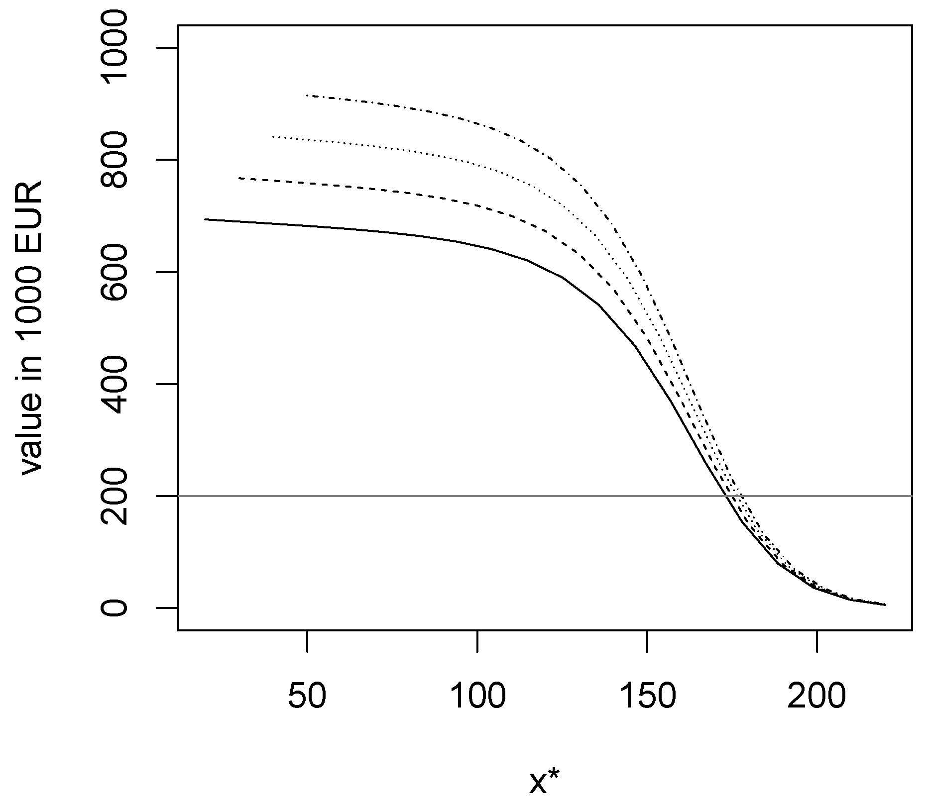
Table 1.
Summary statistics for the 15 min balancing group price per MWh in the German Amprion area, 1 June 2012 to 31 May 2016.
Table 1.
Summary statistics for the 15 min balancing group price per MWh in the German Amprion area, 1 June 2012 to 31 May 2016.
| Min. | 1st Qu. | Median | Mean | 3rd Qu. | Max. |
|---|---|---|---|---|---|
| −6002.00 | 0.27 | 33.05 | 31.14 | 66.97 | 6344.00 |
© 2019 by the authors. Licensee MDPI, Basel, Switzerland. This article is an open access article distributed under the terms and conditions of the Creative Commons Attribution (CC BY) license (http://creativecommons.org/licenses/by/4.0/).
Share and Cite
MDPI and ACS Style
Moriarty, J.; Palczewski, J. Imbalance Market Real Options and the Valuation of Storage in Future Energy Systems. Risks 2019, 7, 39. https://doi.org/10.3390/risks7020039
AMA Style
Moriarty J, Palczewski J. Imbalance Market Real Options and the Valuation of Storage in Future Energy Systems. Risks. 2019; 7(2):39. https://doi.org/10.3390/risks7020039
Chicago/Turabian StyleMoriarty, John, and Jan Palczewski. 2019. "Imbalance Market Real Options and the Valuation of Storage in Future Energy Systems" Risks 7, no. 2: 39. https://doi.org/10.3390/risks7020039
Note that from the first issue of 2016, this journal uses article numbers instead of page numbers. See further details here.